Holographic constraints on Bjorken hydrodynamics at finite coupling

JHEP10(2017)110

Received: September 14, 2017 Accepted: October 7, 2017 Published: October 17, 2017

Holographic constraints on Bjorken hydrodynamics at

finite coupling

Brandon S. DiNunno,a,b,e Saˇso Grozdanov,c Juan F. Pedrazad and Steve Younge a_{Theory Group, Department of Physics, The University of Texas at Austin,}

2515 Speedway, Stop C1608, Austin, TX 78712, U.S.A. b_{Helsinki Institute of Physics, University of Helsinki,}

P.O. Box 64, Helsinki FIN-00014, Finland

c_{Instituut-Lorentz for Theoretical Physics, Leiden University,} Niels Bohrweg 2, Leiden 2333 CA, The Netherlands

d_{Institute for Theoretical Physics, University of Amsterdam,} Science Park 904, 1090 GL Amsterdam, The Netherlands e_{Theory Group, Maxwell Analytics LLC,}

600 Sabine Street, Austin, TX 78701, U.S.A.

E-mail: bsd86@physics.utexas.edu,grozdanov@lorentz.leidenuniv.nl,

jpedraza@uva.nl,scyoung@zippy.ph.utexas.edu

Abstract: In large-Nc conformal field theories with classical holographic duals, inverse coupling constant corrections are obtained by considering higher-derivative terms in the corresponding gravity theory. In this work, we use type IIB supergravity and bottom-up Gauss-Bonnet gravity to study the dynamics of boost-invariant Bjorken hydrodynamics at finite coupling. We analyze the time-dependent decay properties of non-local observ-ables (scalar two-point functions and Wilson loops) probing the different models of Bjorken flow and show that they can be expressed generically in terms of a few field theory pa-rameters. In addition, our computations provide an analytically quantifiable probe of the coupling-dependent validity of hydrodynamics at early times in a simple model of heavy-ion collisheavy-ions, which is an observable closely analogous to the hydrodynamizatheavy-ion time of a quark-gluon plasma. We find that to third order in the hydrodynamic expansion, the convergence of hydrodynamics is improved and that generically, as expected from field theory considerations and recent holographic results, the applicability of hydrodynamics is delayed as the field theory coupling decreases.

Keywords: Holography and quark-gluon plasmas, AdS-CFT Correspondence, Quark-Gluon Plasma

JHEP10(2017)110

1 Introduction 1

2 Hydrodynamics and Bjorken flow 7

3 Gravitational background in Gauss-Bonnet gravity 10

3.1 Static background 11

3.2 Bjorken flow geometry 13

3.3 Solutions 14

3.4 Stress-energy tensor and transport coefficients 15

4 Breakdown of non-local observables 17

4.1 Two-point functions 18

4.1.1 Perturbative expansion: Eddington-Finkelstein vs. Fefferman-Graham 18

4.1.2 Transverse correlator 20

4.1.3 Longitudinal correlator 23

4.2 Wilson loops 29

4.2.1 Transverse Wilson loop 29

4.2.2 Longitudinal Wilson loop 30

5 Discussion 34

A Second order solutions in perturbative Gauss-Bonnet gravity 36

B Metric expansions 37

B.1 Explicit expansions in Fefferman-Graham coordinates 39

C Useful definitions 40

1 Introduction

JHEP10(2017)110

quasiparticles has been firmly established much more recently through the advent of gauge-gravity duality (holography) [25–28]. In infinitely strongly coupled CFTs with a simple holographic dual, the mean-free-time is set by the Hawking temperature of the dual black hole,tmft ∼~/kBT.1 In a CFT in which temperature is the only energy scale, this implies that hydrodynamics universally applies to the IR regime of strongly coupled systems for

ω/T 1, where the frequency scales asω∼1/thyd (and similarly for momenta,q/T 1). A natural question that then emerges is as follows: how does the range of applicability of hydrodynamics depend on the coupling strength of the underlying microscopic quantum field theory? Qualitatively, using simple perturbative kinetic theory arguments (see e.g. a recent work by Romatschke [29] or ref. [30]), one expects the reliability of hydrodynamics to decrease (at some fixedω/T and q/T) with decreasing coupling constantλ. The reason is that, typically, the mean-free-time increases with decreasingλ. From the strongly coupled, non-perturbative side, the same picture recently emerged in holographic studies of (inverse) coupling constant corrections to infinitely strongly coupled systems in [31–34],2 which we will further investigate in this work.

In holography, in the limit of infinite number of colors Nc of the dual gauge theory, inverse ’t Hooft coupling constant corrections correspond to higher derivative gravity α0

corrections to the classical bulk supergravity. In maximally supersymmetric N = 4 Yang-Mills (SYM) theory, dual to the IR limit of ten-dimensional type IIB string theory, the leading-order corrections to the gravitational sector (including the five-form flux and the dilaton), are given by the action [37–41]

SIIB=

1 2κ2

10 Z

d10x√−g

R−1 2(∂φ)

2₋ 1 4·5!F

2 5 +γe

−3

2φW+. . .

, (1.1)

compactified on S5, where γ =α03ζ(3)/8, κ10 ∼1/Nc and the termW is proportional to fourth-power (eight derivatives of the metric) contractions of the Weyl tensor

W =CαβγδCµβγνCαρσµCνρσδ+ 1 2C

αδβγ_C

µνβγCαρσµCνρσδ. (1.2)

The ’t Hooft coupling of the dual N = 4 CFT is related to γ by the following expression:

γ = λ−3/2ζ(3)L6/8, where L is the anti-de Sitter (AdS) length scale. For this reason, perturbative corrections inγ ∼α03 are dual to perturbative corrections in 1/λ3/2.

Another family of theories, which have been proven to be a useful laboratory for the studies of coupling constant dependence in holography, are curvature-squared theo-ries [31–34,42,43] with the action given by

SR2 =

1 2κ2₅

Z

d5x√−g

R−2Λ +L2 α1R2+α2RµνRµν+α3RµνρσRµνρσ

. (1.3)

1_{We will henceforth set}

~=c=kB= 1.

2_{Aspects of the coupling constant dependent quasinormal spectrum inN = 4 theory were first analyzed}

JHEP10(2017)110

theories as invaluable bottom-up constructions for investigations of coupling constant cor-rections on dual observables of hypothetical CFTs.4 From this point of view, it is natural to interpret the αn coefficients as proportional to α0. Since the action (1.3) results in higher-derivative equations of motion, theαn need to be treated perturbatively, i.e. on the same footing as theγ ∼α03 corrections inN = 4 SYM. The latter restriction can be lifted if one instead considers a curvature-squared action with the αn coefficients chosen such thatα1 =−4α2 =α3. The resulting theory, known as the Gauss-Bonnet theory

SGB =

1 2κ2

5 Z

d5x√−g

R+ 12

L2 + λGBL2

2 R

2_−4R

µνRµν+RµνρσRµνρσ

, (1.4)

results in second-derivative equations of motions, therefore enabling one to treat the Gauss-Bonnet coupling, λGB ∈ (−∞,1/4], at least formally, non-perturbatively.5 Even though

this theory is known to suffer from various UV causality problems and instabilities [47–64], one may still treat eq. (1.4) as an effective theory which can, for sufficiently low energy and momentum, provide a well-behaved window into non-perturbative coupling constant corrections to the low-energy part of the spectrum. This point of view was advocated and investigated in [31, 34, 42, 43] where it was found that a variety of weakly coupled properties of field theories, including the emergence of quasiparticles, were successfully recovered not only from the type IIB supergravity action (1.1) but also from the Gauss-Bonnet theory (1.4).6 An important fact to note is that these weakly coupled predictions follow from the theory with anegative λGB coupling (increasing |λGB|).

We can now return to the question of how coupling dependence influences the validity of hydrodynamics as a description of IR dynamics by using the above two classes of top-down and bottom-up higher derivative theories. The first concrete holographic demonstration of the failure of hydrodynamics at reduced (intermediate) coupling was presented in [31]. The same qualitative behaviour was observed in both N = 4 and (non-perturbative) Gauss-Bonnet theory. Namely, as one increases the size of higher derivative gravitational couplings (decreases the coupling in a dual CFT), there is an inflow of new (quasinormal) modes along the negative imaginary ω axis from−i∞. Note that at infinite ’t Hooft coupling λ, these modes are not present in the quasinormal spectrum. However, as λdecreases, the leading new mode on the imaginary ω axis monotonically approaches the regime of small ω/T. In the shear channel,7 which contains the diffusive hydrodynamic mode, the new mode collides with the hydrodynamic mode after which point both modes acquire real parts in

3_{In some cases, such terms can be interpreted as 1/N}

ccorrections rather than coupling constant

correc-tions [44,45]. See also [34] for a recent discussion of these issues.

4_{It is well known that curvature-squared terms appear in various effective IR limits of e.g. bosonic and}

heterotic string theory (see e.g. [46]).

5_{Note that through the use of gravitational field redefinitions, the action (1.3) and any holographic}

results that follow from it can be reconstructed from corresponding calculations inN = 4 theory at infinite coupling (αn= 0) and perturbative Gauss-Bonnet results. See e.g. [42,47].

6_{We refer the readers to ref. [34] for a more detailed review of known causality problems and instabilities}

of the Gauss-Bonnet theory.

7_{See [65] for conventions regarding different channels and the connection between quasinormal modes}

JHEP10(2017)110

the new mode have dispersion relations [31,34]

ω1=−i η ε+Pq

2_{+· · · , (1.5)}

ω2=ωg+i η ε+Pq

2_{+· · · , (1.6)}

where the imaginary gap ωg, the shear viscosity η and energy density ε, and pressure P

depend on the details of the theory [31,34]. Note also that both the IIB coupling γ and the Gauss-Bonnet coupling−λGB have to be taken sufficiently large in order for this effect

to be well described by the small-q expansion (see ref. [34]). In the sound channel,

ω1,2 =±csq−iΓq2+· · · , (1.7) ω3 =ωg+ 2iΓq2+· · ·, (1.8)

wherecs= 1/ √

3 is the conformal speed of sound and Γ = 2η/3 (ε+P). In both channels, it is clear that the IR is no longer described by hydrodynamics. To quantify this, it is natural to define a critical coupling dependent momentum qc(λ) at which Im|ω1(qc)|= Im|ω2(qc)| in the shear channel, and Im|ω1,2(qc)| = Im|ω3(qc)| in the sound channel. With this definition, hydrodynamic modes dominate the IR spectrum for frequencies ω(q), so long as q < qc(λ). To leading order in the hydrodynamic approximation, in N = 4 theory, qc scales asqc ∼0.04T /γ∼0.28λ3/2T, while in the Gauss-Bonnet theory,qc ∼ −3.14T /λGB.

Even though these scalings are approximate, they nevertheless reveal what one expects from kinetic theory: the applicability of hydrodynamics is limited at weaker coupling by a coupling dependent scaling whereas at strong coupling, hydrodynamics is only limited to the region of small q/T, independent ofλ1.8

Understanding of hydrodynamics has been important for not only the description of everyday fluids and gases, but also a nuclear state of matter known as the quark-gluon plasma that is formed after collisions of heavy ions at RHIC and the LHC. Hydrodynam-ics becomes a good description of the plasma after a remarkably short hydrodynamization timethyd ∼1−2 fm/c measured from the moment of the collision [66–71]. In holography, heavy ion collisions have been successfully modelled by collisions of gravitational shock waves [72–79], including the correct order of magnitude result for the hydrodynamization time (at infinite coupling). Coupling constant corrections to holographic heavy ion colli-sions were studied in perturbative curvature-squared theories (Gauss-Bonnet) in [32], which found that for narrow and wide gravitational shocks, respectively, the hydrodynamization time is

thydThyd = 0.41−0.52λGB+O(λ2GB), thydThyd = 0.43−6.3λGB+O(λ

2

GB),

(1.9)

where Thyd is the temperature of the plasma at the time of hydrodynamization. For λGB=−0.2, which corresponds to an 80% increase in the ratio of shear viscosity to entropy

density, we thus find a 25% and 290% increase in the hydrodynamization time [32]. Thus,

8_{In kinetic theory (within relaxation time approximation), the hydrodynamic pole does not collide with}

JHEP10(2017)110

thyd was found to increase for negative values of λGB, which is consistent with expectations

of the behavior of hydrodynamization at decreased field theory coupling. Consistent with these findings, the investigation of [33, 80] further revealed that for negative λGB, the

isotropization time of a plasma also increased, again reproducing the expected trend of transitioning from infinite to intermediate coupling.

In this paper, we continue the investigation of coupling constant dependent physics by studying the simplest hydrodynamic model of heavy ions — the boost-invariant Bjorken flow [81] — in higher derivative bulk theories of gravity. The Bjorken flow has widely been used to study the evolution of a plasma (in the mid-rapidity regime) after the collision. While the velocity profile of the solution is completely fixed by symmetries, relativistic Navier-Stokes equations need to be used to find the energy density, which is expressed as a series in inverse powers of the proper time τ. The details of the solution will be described in section 2.

In N = 4 SYM at infinite coupling, the energy density of the Bjorken flow to third order in the hydrodynamic expansion (ideal hydrodynamics and three orders of gradient corrections) takes the following form [82–88]:

hTτ τi=ε(τ) = 6N_c2

π2 w4 τ4/3

1− 1 3wτ2/3 +

1 + 2 ln 2 72w2_τ4/3 −

3−2π2−24 ln 2+24 ln22 3888w3_τ2

, (1.10)

wherewis a dimensionful constant.9 Physically, the energy density of the Bjorken flow must be a positive and monotonically decreasing function of the proper time τ, capturing the late-time expansion and cooling of the fluid. For a conformal, boost-invariant system, the energy density (1.10) uniquely determines all the components of the stress-energy tensor. Energy conditions then imply that the solution becomes unphysical at sufficiently early times, when (1.10) is negative. For instance, by considering the first two terms in (1.10), it is clear that the solution becomes problematic at times τ < τ_hyd1st, where

τ_hyd1stw3/2 = 0.19. (1.11)

Physically, the reason is that for τ < τhyd, the first viscous correction becomes large and the hydrodynamic expansion breaks down, making the Bjorken flow unphysical.10 Ref. [90] further analyzed the evolution of non-local observables in a boost-invariant Bjorken plasma, finding stronger constraints on the value of initialτ for the Bjorken solution. For instance, equal-time two-point functions and space-like Wilson loops are expected to relax at late times as

hO(x)O(x0)i hO(x)O(x0_)i|

vac

∼e−∆f(τ w3/2), hW(C)i

hW(C)i|vac ∼e−

√

λg(τ w3/2₎

, (1.12)

for some f and g such that f(τ w3/2) → 0 and g(τ w3/2) → 0 as τ → ∞. In the hydro-dynamic regime, both f and g must be positive and monotonically decreasing functions

9_{Other conventions that appear in the literature use Λ =}2w π or=

3w4 4 .

10_{Higher-order hydrodynamic corrections are expected to improve this bound. However, since}

hydrody-namics is anasymptoticexpansion, there should be an absolute lower bound for the regime of validity of hydrodynamics (at all orders). Ref. [89] estimated this bound to be τhydThyd ∼0.6 by analyzing a large

JHEP10(2017)110

from above to the corresponding vacuum values. Such exponential decays have indeed been observed from the full numerical evolution in shock wave collisions [91, 92]. The interest-ing point here is that, if we were to truncate the hydrodynamic expansion to include only the first few viscous corrections, then f and g may become negative or non-monotonic at someτcrit> τhyd, imposing further constraints on the regime of validity of hydrodynamics. In [90], it was found that a much stronger constraint (approximately 15 times stronger than (1.11)) for first-order hydrodynamics comes from the longitudinal two-point function:

τ_crit1stw3/2= 2.83, (1.13)

while for Wilson loops, the constraint was weaker:

τ_crit1stw3/2= 0.65. (1.14)

In addition, ref. [90] also studied the evolution of entanglement (or von Neumann) entropy in a Bjorken flow, but found that the bound obtained in that case was equal toτ_hyd1st given by eq. (1.11), i.e. weaker than the two constraints above. The reason for this equality is that in the late-time and slow-varying limit considered for the computation, the entanglement entropy satisfies the so-called first law of entanglement,

SA(τ) =ε(τ) VA TA

, (1.15)

whereVA is the volume of the subsystem and TA is a constant that depends on its shape. Such a law holds for arbitrary time-dependent excited states provided the evolution of the system is adiabatic with respect to a reference state [93].

In this paper, we ask how higher-order hydrodynamic and coupling constant correc-tions affect the critical time τcrit after which the Bjorken flow yields physically sensible observables. In particular, we extend the analysis of [90] focusing on equal-time two-point functions and expectation values of Wilson loops. From the point of view of our discus-sion regarding viscous corrections and their role in keeping ε(τ) positive, it seems clear that at decreased coupling, when the viscosity η becomes larger, the applicability of the Bjorken solution should become relevant at larger τ. Our calculations provide further details regarding the applicability of hydrodynamics. As a result, we will be computing an observable that is related to a coupling-dependent hydrodynamization time [32], but is analytically-tractable and therefore significantly simpler to analyze, albeit for realistic applications limited to the applicability of the Bjorken flow model. In this way, we obtain new holographic coupling-dependent estimates for the validity of hydrodynamics, analo-gous to the statement of eq. (1.9), which allow us to compare top-down and bottom-up higher derivative corrections.

JHEP10(2017)110

two-point function, i.e. with spatial insertions along the boost-invariant flow direction. For the two higher-derivative theories, to first order in the coupling and to second order in the hydrodynamic expansion,

τ_crit2ndw3/2 = 1.987 + 275.079γ+O(γ2) = 1.987 + 41.333λ−3/2+O(λ−3), (1.16)

τ_crit2ndw3/2 = 1.987−14.876λGB+O(λ

2

GB), (1.17)

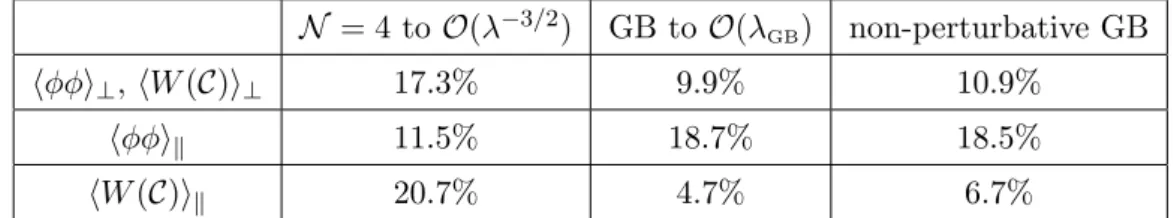
where τcrit is the initial critical proper-time. At γ = 6.67 ×10−3 (λ = 7.98, having set L = 1) and at λGB = −0.2 (each increasing η/s by 80%), we find that τ_crit2ndw3/2

increases by 92.3% and by 150% in N = 4 and a linearized dual of Gauss-Bonnet theory, respectively (see tables1and 2for other numerical estimates). In a fully non-perturbative Gauss-Bonnet calculation, the increase is instead found to be 145%, which shows a rather quick convergence of the perturbative Gauss-Bonnet series for this observable to the full result at λGB = −0.2 (see also [32]). Thus, our results lie inside the interval of increased

hydrodynamization time found in narrow and wide shocks obtained from non-linear shock wave simulations [32].

The paper is structured as follows: in section2, we discuss higher-order hydrodynamics and details of the hydrodynamic Bjorken flow solution, including all necessary holographic transport coefficients that enter into the solution. In section 3, we discuss the construction of holographic dual geometries to Bjorken flow. We focus in particular on the case of the Gauss-Bonnet theory which, to our understanding, has not been considered in previous literature.11 In section4, we analyze the relaxation properties of two-point functions and Wilson loops, extracting the relevant critical times at which the hydrodynamic approxima-tion breaks down. Finally, secapproxima-tion 5 is devoted the discussion of our results.

2 Hydrodynamics and Bjorken flow

We begin by expressing the equations that describe the boost-invariant evolution of charge-neutral, conformal relativistic fluids, which will be studied in this work. In the absence of any external sources, the equations of motion (relativistic Navier-Stokes equations) follow from the conservation of stress-energy

∇_aTab= 0. (2.1)

The constitutive relations for the stress-energy tensor of a neutral, conformal (Weyl-covariant) relativistic fluid can be written as (see e.g [97])

Tab =εuaub+P∆ab+ Πab, (2.2)

where we have chosen to work in the Landau frame. The transverse projector ∆ab is defined as ∆ab ≡ gab+uaub, with ua being the velocity field of the fluid flow. In four spacetime dimensions, the pressure P and energy density ε are related by the conformal

11_{The background for type IIB supergravityα}0

JHEP10(2017)110

a gradient expansion (in gradients ofuaand a scalar temperature field). To third order in derivatives [94,98,99],

Πab =−ησab+ητΠ

h_Dσabi₊1 3σ

ab_{(∇ ·u)}

+κhRhabi−2ucRchabidud i

+λ1σhacσb ic_+λ

2σhacΩb ic_+λ

3ΩhacΩb ic₊

20 X

i=1

λ(3)_i Oab_i , (2.3)

where we have used the longitudinal derivative D≡ua∇a and a short-hand notation

Ahabi≡ 1 2∆

ac_∆bd_(A

cd+Adc)− 1 3∆

ab_∆cd_A

cd≡hAabi, (2.4)

which ensures that any tensorAhabi is by construction transverse,uaAhabi= 0, symmetric and traceless, gabAhabi= 0. The tensor σab is a one-derivative shear tensor

σab= 2h∇aubi. (2.5)

The vorticity Ωµν is defined as the anti-symmetric, transverse and traceless tensor

Ωab = 1 2∆

ac_∆bd_(∇

cud− ∇duc) . (2.6)

The transport coefficients appearing in (2.3) are the shear viscosity η, 5 second order coefficients ητΠ,κ,λ1,λ2,λ3, and 20 (subject to potential entropy constraints) conformal third order transport coefficients λ(3)_i , which multiply 20 linearly independent, third order Weyl-covariant tensors Oab

i that can be found in [94].

The boost-invariant Bjorken flow [81] is a solution to the hydrodynamic equations (eq. (2.1)), and has been widely used as a simple model of relativistic heavy ion colli-sions (see [77]). Choosing the direction of the beam to be the z axis, the Bjorken flow is boost-invariant along z, as well as rotationally and translationally invariant in the plane perpendicular to z (denoted by ~x⊥). By introducing the proper time τ = √t2_−z2 _and the rapidity parameter y = arctanh(z/t), the velocity field, which is completely fixed by symmetries, and the flat metric can be written as

ua=uτ, uy, ~u⊥= (1,0,0,0), (2.7)

ηabdxadxb =−dτ2+τ2dy2+d~x2⊥. (2.8)

Note that the solution is also invariant under discrete reflectionsy → −y. What remains is for us to find the solution for the additional scalar degree of freedom that is required to fully characterize the flow. In this case, it is convenient to work with a proper time-dependent energy density ε(τ) and write eq. (2.1) as in [98]:

JHEP10(2017)110

of ∇aub is∇yuy =∇⊥yuy =τ, eq. (2.9) then gives

∂τε+ 4 3

ε τ +τΠ

yy_{= 0, (2.10)}

with Πyy from eq. (2.3) expanded as

Πyy=−4η 3

1

τ3−

8ητΠ 9 −

8λ1 9

1

τ4− "

λ(3)₁

6 + 4λ(3)₂

3 + 4λ(3)₃

3 + 5λ(3)₄

6 + 5λ(3)₅

6 + 4λ(3)₆

3

−λ (3) 7 2 +

3λ(3)₈

2 +

λ(3)₉

2 − 2λ(3)₁₀

3 − 11λ(3)₁₁

6 −

λ(3)₁₂

3 +

λ(3)₁₃

6 −λ (3) 15

# 1

τ5+O τ −6

. (2.11)

Each transport coefficient appearing in (2.11) can only be a function of the single scalar degree of freedom — the energy density — with dependence on εdetermined uniquely by its conformal dimension under local Weyl transformations [94,98]:

η=Cη¯ε

C 3/4

, ητΠ=Cη¯τ¯Π ε

C 1/2

, λ1 =Cλ¯1 ε

C 1/2

, λ(3)_n =C¯λ(3)_n ε C

1/4 ,

(2.12) where C, ¯η, ¯τΠ and ¯λ(3)n are constants. Finally, the Bjorken solution to eq. (2.1) for the energy density, expanded in powers of τ, becomes

ε(τ)

C =

1

τ2−ν −2¯η 1

τ2 +

3¯η2

2 − 2¯ητ¯Π

3 + 2¯λ1

3

1

τ2+ν (2.13)

− "

¯

η3

2 − 7¯η2τ¯Π

9 +

7¯η¯λ1 9 +

¯

λ(3)₁

12 + 2¯λ(3)₂

3 + 2¯λ(3)₃

3 + 5¯λ(3)₄

12 + 5¯λ(3)₅

12 + 2¯λ(3)₆

3

− ¯λ (3) 7 4 +

3¯λ(3)₈

4 + ¯

λ(3)₉

4 − ¯

λ(3)₁₀

3 − 11¯λ(3)₁₁

12 − ¯

λ(3)₁₂

6 + ¯

λ(3)₁₃

12 − ¯

λ(3)₁₅

2 #

1

τ2+2ν +O τ −2−3ν

,

with ν = 2/3. Terms at order O τ−2−3ν

are controlled by the hydrodynamic expansion to fourth order, which is presently unknown.

In theories of interest to this work, namely in the N = 4 supersymmetric Yang-Mills theory and in hypothetical duals of curvature-squared gravity, all first- and second-order transport coefficients are known. InN = 4 theory (cf. eq. (1.1)), the relevant expressions, including the leading-order ’t Hooft coupling corrections are [42,100–106]

η= π 8N

2 cT3

1 +135ζ(3)

8 λ

−3/2_{+. . .}

, (2.14)

τΠ=

(2−ln 2) 2πT +

375ζ(3) 32πT λ

−3/2_{+. . . , (2.15)}

λ1 = N_c2T2

16

1 +175ζ(3)

4 λ

−3/2_{+. . .}

JHEP10(2017)110

to first order [42],

η = r 3 + 2κ2 5

(1−8 (5α1+α2)) +O(α2i), (2.17)

ητΠ=

r₊2 (2−ln 2) 4κ2₅

1− 26

3 (5α1+α2)

−r 2

+(23 + 5 ln 2)

12κ2₅ α3+O(α 2

i), (2.18)

λ1 = r2₊

4κ2 5

1−26

3 (5α1+α2)

− r 2 + 12κ2

5

α3+O(α2i), (2.19)

wherer+is the position of the event horizon in the bulk, which depends on all threeαi (see ref. [42]). Finally, in a dual of the Gauss-Bonnet theory (cf. eq. (1.4)) all first- and second-order transport coefficients are known non-perturbatively in the coupling λGB [34,42,43],

η = √

2π3 κ2₅

T3_γ2

GB

(1 +γGB)

3/2 , (2.20)

τΠ= 1 2πT

1

4(1 +γGB)

5 +γGB−

2 γGB −1 2ln

2 (1 +γGB) γGB

, (2.21)

λ1 = η

2πT

(1 +γGB) 3−4γGB+ 2γGB3

2γ2

GB

!

, (2.22)

where we have defined the coupling γGB as

γGB ≡

p

1−4λGB. (2.23)

The relevant linear combination of the third-order transport coefficients appearing in (2.13) is to date only known inN = 4 theory at infinite coupling. The expression was found in [94] by using the holographic Bjorken flow result of [82–88] for ε(τ) stated in eq. (1.10), giving

λ(3)₁

6 + 4λ(3)₂

3 + 4λ(3)₃

3 + 5λ(3)₄

6 + 5λ(3)₅

6 + 4λ(3)₆

3 −

λ(3)₇

2

+3λ (3) 8 2 +

λ(3)₉

2 − 2λ(3)₁₀

3 − 11λ(3)₁₁

6 −

λ(3)₁₂

3 +

λ(3)₁₃

6 −λ (3) 15 =

N_c2T

648π 15−2π

2_{−45 ln 2+24 ln}2₂

+· · ·, (2.24)

where the ellipsis indicates unknown coupling constant corrections.

In this work, we will not look beyond third-order hydrodynamics. What is important to note is that the gradient expansion is believed to be an asymptotic expansion, similar to perturbative expansions. As a result, the Bjorken expansion in proper time formally has a zero radius of convergence [95]. In practice, this means that at some order, the expansion in inverse powers ofτ breaks down and techniques of resurgence are required for analyzing long-distance transport (see e.g. [95,107–112]).

3 Gravitational background in Gauss-Bonnet gravity

JHEP10(2017)110

order in the hydrodynamic series.

• α0-corrections. Bjorken flow inN = 4 SYM with first-order ’t Hooft coupling correc-tions, α03∼1/λ3/2, expanded to second order in the hydrodynamic series.

• λGB-corrections. Bjorken flow in a hypothetical dual of Gauss-Bonnet theory with

λGB coupling corrections, expanded to second order in the hydrodynamic series.

In the first case, the holographic dual geometry is well known (see refs. [82–88]). What one finds is that in the near-boundary region, which is the only region relevant for com-puting the non-local observables studied in this paper (two-point correlators of operators with large dimensions and Wilson loops), the geometries are specified by symmetry and (relevant order) hydrodynamic transport coefficients.12 _{As we will see, the same}

conclu-sions can also be drawn in higher-derivative theories. As a check, we derive here the full geometric Bjorken background in non-perturbative Gauss-Bonnet theory. All details of the perturbative calculations in Type IIB supergravity withα0 corrections will be omitted, but we refer the reader to [96] for the explicit derivation.

3.1 Static background

Equations of motion for Gauss-Bonnet gravity in five dimensions can be derived from the action (1.4) and take the following form:

Rµν− 1 2gµν

R+ 12

L2 + λGBL2

2 LGB

+λGBL2Hµν = 0, (3.1)

where

LGB =RµναβRµναβ−4RµνRµν+R2,

H_µν =RµαβρRναβρ−2RµανβRαβ −2RµαRνα+RµνR .

This set of differential equations admits a well-known (static) asymptotically AdS black brane solution:

ds2=−r 2_f(r)

˜

L2 dτ

2₊ L˜2 r2_f(r)dr

2₊ r2 ˜

L2d~x

2_{, (3.2)}

with the emblackening factor

f(r) = 1 2λGB

˜

L2 L2



1− s

1−4λGB

1−r

4 h r4



. (3.3)

In the near-boundary limit, the asymptotically AdS region exhibits the following scaling:

ds2 r→∞ =

˜

L2 r2dr

2₊ r2 ˜

L2 −dτ

2_+d~x2 =

˜

L2 r2dr

2₊ r2 ˜

L2ηabdx

a_dxb_{, (3.4)}

JHEP10(2017)110

set by the cosmological constant, L, via

˜

L2 = L 2

2

1 +p1−4λGB

= L

2

2 (1 +γGB). (3.5)

The Hawking temperature, entropy density and energy density of the dual theory are then given by13

T = rh

πL2 , (3.6)

s= 4

√ 2π

(1 +γGB)3/2κ2₅

r_h L

3

, (3.7)

ε= 3P = 3

4T s . (3.8)

In what follows, we will setL= 1 unless otherwise stated.

To make the metric manifestly boost-invariant along the spatial coordinatez, we trans-form (3.2) by introducing a proper time coordinate τ = √t2_−z2_{. Next, we perform an} additional coordinate transformation to write the metric in terms of ingoing Eddington-Finkelstein (EF+) coordinates with

τ →τ+−L˜2

Z r _d˜r

˜

r2_f(˜r), (3.9)

which gives the metric

ds2 =−r 2

˜

L2f(r)dτ 2

++ 2dτ+dr+ r2

˜

L2d~x

2_{. (3.10)}

It should be noted that the EF+time, τ+, mixes the proper time,τ, andr in the bulk. At the boundary, however,

lim

r→∞τ+=τ . (3.11)

A static black brane with a constant temperature cannot be dual to an expanding Bjorken fluid, which has a temperature that decreases with the proper time, Tfluid∼τ−1/3. As in the fluid-gravity correspondence [99], where the black brane is boosted along spatial directions, here, one may make an informed guess and allow for the horizon to become time-dependent by substituting

rh →wτ −1/3

+ , (3.12)

where w is a constant and τ+ is the fluid’s proper time at the boundary. The Hawking temperature is then

T = w

πL2τ −1/3

+ , (3.13)

and the static black brane metric (3.10) takes the form

ds2 =−r 2

˜

L2

1 1−γGB

"

1−γGB

s

1−

1− 1

γ2

GB

w4

v4 #

dτ₊2 + 2dτ+dr+ r2

˜

L2d~x

2_{, (3.14)}

13_{We note that our black brane background can be put into the form given by eq. (2.2) of [34] by a}

JHEP10(2017)110

v≡rτ₊1/3. (3.15)

Of course, as in the fluid-gravity correspondence, eq. (3.14) is not a solution to the Gauss-Bonnet equations of motion. As will be shown below, however, the background solution asymptotes to (3.14) at late times, i.e. eq. (3.14) is (approximately) dual to Bjorken flow in the regime dominated by ideal hydrodynamics.

3.2 Bjorken flow geometry

The full (late-time) geometry is systematically constructed following the procedure outlined in ref. [113] (see also [114]). In EF+coordinates, the most general metric respecting the symmetries of Bjorken flow is

ds2=−r 2

˜

L2adτ 2

++ 2dτ+dr+ 1 ˜

L2

˜

L2+rτ+ 2

e2(b−c)dy2+ r 2

˜

L2e c_dx2

⊥, (3.16)

wherea,b,c are functions ofr andτ+ and our boundary geometry is expressed in proper time-rapidity coordinates (see the discussion above eq. (2.8)).

At late times, the equations of motion (3.1) can be solved order-by-order in powers of

τ₊−2/3, provided theτ+ → ∞expansion is carried out holding v≡rτ 1/3

+ fixed. To perform the late time expansion, we will change coordinates from {τ+, r} → {v, u}, where

v≡rτ₊1/3, u≡τ₊−2/3, (3.17)

and assume the metric functions a,band c can be expanded as

a(u, v) =a0(v) +a1(v)u+a2(v)u2+. . . . (3.18)

We then solve the equations order-by-order in powers of u and impose Dirichlet boundary conditions (at the boundary) at every order:

lim

v→∞a0 = 1, lim

v→∞{ai>0, bi, ci}= 0. (3.19) At a given order, i, the equations of motion form a system of second-order differential equations for ai, bi and ci along with two constraint equations. We therefore have six integration constants at each order. One integration constant is related to a residual diffeomorphism invariance of our metric under the coordinate transformation [113]

r→r+f(τ+), (3.20)

JHEP10(2017)110

remaining integration constants are specified by the two constraint equations. For i >0, one of the constraint equations can specify a constant at order i, while the other specifies a constant at orderi−1.

3.3 Solutions

We now present the full zeroth- and first-order solutions in the late-time (hydrodynamic gradient) expansion. At second order, we were unable to find closed-form solutions an-alytically that would extend throughout the entire bulk. However, sufficiently complete solutions for the purposes of this work can be found non-perturbatively in λGB near the

boundary, or perturbatively in the full bulk.

Zeroth order. At zeroth order in the hydrodynamic expansion (ideal fluid order), the equations of motion are solved by15

a0=

1 1−γGB

"

1−γGB

s

1−

1− 1

γ2

GB

w4

v4 #

,

b0= 0,

c0= 0. (3.21)

One can see immediately that the zeroth-order solution is the boosted black brane metric given by eq. (3.14). Near the boundary we find

a0= 1−

1 +γGB

2γGB

w

v 4

+O(v−5),

b0= 0,

c0= 0. (3.22)

First order. At first (dissipative) order, our equations of motion are solved by

a1 =

γGB(1 +γGB)

3

1 1−γGB

1

v + v G

w3 v3 −

1 1−γGB

,

b1 = 0,

c1 =

γGB(1 +γGB)

3

Z v _d˜v

˜

v2

1 ˜

v2_−γ

GBG

1−(1−γGB)

w

˜

v 3

G−˜v2

, (3.23)

where

G(v)≡v2 s

1−

1− 1

γ2

GB

w4

v4 . (3.24)

For simplicity, here we have presented c1 in an integral representation. An explicit eval-uation of the integral would result in an Appell hypergeometric function (see ref. [34]).16

14

With the next section in mind, we require lim

v→w+∂vci<∞. 15

We note that this is not the most general solution to the equations of motion at this order — there is an additional nonphysical integration constant corresponding to a gauge degree of freedom. A simple coordinate transformation [113] brings the solution into the form presented here. Similar remarks apply for the first-order solution.

16

We note that upon integration, the integration constant is fixed by requiring lim

JHEP10(2017)110

a1=

γGB(1 +γGB)

3w

w

v 4

+O(v−5),

b1= 0,

c1=

γGB(1 +γGB)

12w

w

v 4

+O(v−5). (3.25)

Second order. As in Gauss-Bonnet fluid-gravity calculations [34], at second order in the hydrodynamic expansion, one is required to solve non-homogeneous differential equations with sources depending on complicated expressions involving Appell hypergeometric func-tions. For this reason, we were only able to find non-perturbative solutions (in λGB) near

the boundary and solve the full equations perturbatively. Near the boundary we find

a2 =A2 w

v 4

+O(v−5),

b2 =O(v−5),

c2 =C2 w

v 4

+O(v−5), (3.26)

whereA2 andC2 are, as yet, unspecified constants. To determine them, we would need to know the full bulk solutions and the constants would then follow from horizon regularity. Instead, as will be shown below, we will use known properties of the dual field theory (the transport coefficients and energy conservation) to show that they must take the following values:

A₂=− 1 72w2

1 +γGB γGB

6 +γ_GB2 (1 +γGB)(9γGB−11) + 2γGB2 ln

2 + 2

γGB

,

C₂= A2 2 .

Full perturbative first-order (inλGB) solutions are presented in appendix A. Here, we only

state their near-boundary forms:

a2=− w2

18v4

1 + 2 ln 2−6λGB(1 + ln 2)

+O(v−5),

b2=O(v−5),

c2=− w2

36v4

1 + 2 ln 2−6λGB(1 + ln 2)

+O(v−5). (3.27)

3.4 Stress-energy tensor and transport coefficients

We can now compute the boundary stress-energy tensor by following the well-known holo-graphic procedure (see e.g. [34, 115, 116]), which we review here. First, we introduce a regularized boundary located at r = r0 = const. The induced metric on the regularized boundary is given byγµν ≡gµν−nµnν, wherenµ≡δµr/

√

grr _{is the outward-pointing unit} vector normal to the r=r0 hypersurface. The boundary stress-energy tensor is then

Tµν = 1

κ2 5

r₀2

˜

L2

Kµν −Kγµν+ 3λGBL2

Jµν −

1 3J γµν

+δ1γµν+δ2G(γ)µν

r0→∞

JHEP10(2017)110

curvature17

Kµν =− 1

2(∇µnν +∇νnµ), (3.29)

K =gµνKµν,Jµν is defined by

Jµν ≡ 1

3 2KKµρK ρ

ν+KρσKρσKµν−2KµσKσρKρν−K2Kµν

, (3.30)

and J = gµνJµν. The constants δ1 and δ2, fixed by holographic renormalization, are given by

δ1 =− √

2

2 +γGB

√

1 +γGB

, δ2 =

(2−γGB)

2√2 p

1 +γGB. (3.31)

For the background derived in section3.3, the non-zero components of the four dimensional boundary stress-energy tensor, Tab, are found to be

Tτ+τ+ =

3√2w4

(1 +γGB)3/2κ2₅

τ−4/3−2γ 2

GB

3w τ

−2_{− A} 2

2γGB

1 +γGB

τ−8/3

,

Tyy =

3√2w4 (1 +γGB)3/2κ2₅

1 3τ

2/3₋2γGB2

3w −

2γGB

3 _A

2+ 8C2 1 +γGB

τ−2/3

,

Tx⊥x⊥ =

3√2w4

(1 +γGB)3/2κ2₅

1 3τ

−4/3₋2γGB

3 _A

2−4 C2 1 +γGB

τ−8/3

, (3.32)

where we identify τ+ with the proper time, τ, at the boundary. Before analyzing Tab, we note three immediate observations:

1. Tab is traceless:

ηabTab = 0 (3.33)

withηab given by eq. (2.8).

2. Conservation implies a relationship betweenA2 and C2:

∂aTab= 0 =⇒ C2 = A₂

2 . (3.34)

3. The stress-energy tensor is completely specified by a single time-dependent function,

ε(τ)≡Tτ+τ+:

Tτ+τ+ =ε , Tyy =−τ

2_{(τ ∂}

τε+ε) , Tx⊥x⊥ =ε+

1

2τ ∂τε . (3.35)

The three properties above are the defining properties of the hydrodynamic description of a relativistic, conformal Bjorken fluid. The only thing that remains to be specified is a single integration constant A₂ (see discussion below eq. (3.26)).

17_Here,∇

JHEP10(2017)110

second order in the hydrodynamic gradient expansion as

ε(τ) = C

τ4/3 1−2 ¯

η τ2/3 +

¯ Σ₍₂₎

τ4/3 !

, (3.36)

where ¯Σ(2)represents the relevant linear combination of second-order transport coefficients:

¯ Σ(2) =

3¯η2

2 − 2¯ητ¯II

3 + 2¯λ1

3 . (3.37)

By comparing the energy density of the Gauss-Bonnet fluid derived in the previous section with that of the Bjorken fluid, we identify

C = 3

√ 2w4

(1 +γGB)3/2κ2₅

, η¯= γ 2

GB

3w , Σ¯(2) =−A2

2γGB

1 +γGB

. (3.38)

At zeroth order in the hydrodynamic expansion, the energy density of our plasma is, as required,

ε0 = C τ4/3 =

3√2π4T4

(1 +γGB)3/2κ2₅

, (3.39)

where we have used eq. (3.13) to express our answer in terms of T. The shear viscosity is then

η=Cη¯ε

C 3/4

= √

2π3 κ2₅

T3γ2GB

(1 +γGB)3/2

, (3.40)

which agrees with eq. (2.20). At second order, we find

λ1−ητII =C λ¯1−η¯τ¯II ε

C 1/2

, (3.41)

matches the known result (see eqs. (2.20)–(2.22)),

λ1−ητII = √

2π2

8κ2₅

T2

(1 +γGB)3/2

6 +γ2GB

(3γGB−2)γGB−11

+ 2γGB2 ln

2 + 2

γGB

provided

A2 =− 1 72w2

1 +γGB γGB

6 +γGB2 (1 +γGB)(9γGB−11) + 2γGB2 ln

2 + 2

γGB

. (3.42)

Collecting our results, the energy density, as a function of proper time, takes the final form:

ε(τ) = 3 √

2 (1 +γGB)3/2κ2₅

w4

τ4/3 1− 2γGB2

3w τ

−2/3

+ 1 36w2

6 +γGB2 (1 +γGB)(9γGB−11) + 2γ

2

GBln

2 + 2

γGB

τ−4/3

. (3.43)

4 Breakdown of non-local observables

JHEP10(2017)110

4.1 Two-point functions

According to the holographic dictionary [117,118], bulk fieldsφare dual to gauge-invariant operators O with conformal dimension ∆, specified by their spin s, the mass m and the number of dimensions d. For scalar fields, the relation is given by ∆(∆−d) =m2. The equivalence between the two sides of the correspondence can be made more precise by the identification:

Z_Bulk[φ] = D

eRddxφ(x)O(x)E

CFT. (4.1)

The left-hand-side of the above equation is the bulk partition function, where we impose the boundary condition φ→ d−∆φ. The right-hand-side is the generating functional of correlation functions of the CFT, where the boundary valueφ acts as a source of the dual operator O. The equivalence (4.1) becomes handy by treating the bulk path integral in the saddle point approximation. In this regime, the above relation becomes

Son-shell[φ] =−ΓCFT[φ], (4.2)

where on the left-hand side we have the bulk action evaluated on-shell and the right-hand side is the generating functional of connected correlation functions of the CFT. For instance, two-point functions can be computed by differentiating two times with respect to the source:

hO(x)O(x0)i=− δSon-shell

δφ(x)δφ(x0)

φ=0

. (4.3)

For operators with large conformal dimension ∆ (or equivalently, bulk fields with large massm) the above problem simplifies even further. It can be shown that, in this limit, the relevant two-point functions reduce to the computation of geodesics in the given background geometry [119,120], i.e.

hO(x)O(x0)i ∼e−∆Sreg(x,x0)_{, (4.4)}

whereS_regis the regularized length of a geodesic connecting the boundary points xandx0.

4.1.1 Perturbative expansion: Eddington-Finkelstein vs. Fefferman-Graham

We can now compute the late-time behavior of scalar two-point functions probing the out-of-equilibrium Bjorken flow. In order to do so we will follow the approach of [90].18 Consider the functional L[φ(y);α] for the geodesic length, i.e. S ≡R

dyL[φ(y);α]. Here,

φ(y) denotes collectively all of the embedding functions,yis the affine parameter andαis a small parameter related to the hydrodynamic gradient expansion in which the perturbation is carried out. Its precise definition will be given below. We can expand bothLandφ(y) as:

L[φ(y);α] =L(0)[φ(y)] +αL(1)[φ(y)] +O(α2),

φ(y) =φ(0)(y) +αφ(1)(y) +O(α2). (4.5)

The functions φ(n)(y) can in principle be found by solving the geodesic equation order-by-order inα. However, the embedding equations are in most cases highly non-linear making

JHEP10(2017)110

S_on-shell(x, x0) = Z

dyL(0)[φ(0)(y)] +α Z

dyL(1)[φ(0)(y)]

+α Z

dy φ(1)_i (y)

d dy

∂L(0) ∂φ0_i(y) −

∂L(0) ∂φi(y)

φ(0)

+· · · ,

(4.6)

so we only needφ(0)(y) to obtain the first correction to the geodesic length.

Let us now discuss the expansion parameter α in more detail. In particular, what we will see is that there is a natural choice forαdepending on whether we work in Eddington-Finkelstein or Fefferman-Graham coordinates, so we must proceed with some care before we interpret our results.19 Let us start with the Fefferman-Graham expansion, which was first considered in [90]. In this case, the metric coefficients can be expanded as in eq. (B.8) so each hydrodynamic order is suppressed by a factor of the dimensionless quan-tity ˜u=τ−2/3w−1, wherewis the same dimensionful parameter that appears in the energy density. On the other hand, the near-boundary expansion stipulates that we can alterna-tively expand all metric coefficients in powers of ˜v≡zτ−1/3w. This is the expansion that will be relevant for our perturbative calculation (4.6). Notice that when ˜v→0, we recover pure AdS, for which the embedding function φ(0)(y) is analytically known. The first cor-rection in this expansion enters at order O(˜v4) so we can identifyα∼v˜4. Now, according to the UV/IR connection [122–124], the bulk coordinate z can roughly be mapped to the length scale z∼`in the boundary theory. In our setup, the only length scale of the prob-lem is given by the separation the two points (x, x0) so`∼∆x≡ |x−x0|.20 _{Therefore, in}

terms of CFT data, our expansion parameter in Fefferman-Graham coordinates is given by

α=`4τ−4/3w4 (Fefferman-Graham). (4.7)

As mentioned already in appendix B, the leading correction to the metric in the near-boundary expansion receives contributions at all orders in hydrodynamics, so one can obtain non-trivial results by studying contributions to the two-point correlators to only first order. For instance, as found in ref. [90], in order to have a well behaved late-time relaxation of longitudinal two-point functions, first-order hydrodynamics puts a constraint on the regime of validity of ˜u. Namely, the approximation breaks down when21

˜

u >1/2 =⇒ τ < τ_crit1st = 23/2w−3/2 ≈2.828w−3/2. (4.8)

In this work, we are interested in studying both i) higher order hydrodynamic corrections and ii) (inverse) coupling constant corrections in the N = 4 plasma and a hypothetical dual of Gauss-Bonnet theory.

In Eddington-Finkelstein coordinates, the hydrodynamic expansion is performed in terms of u, and the near boundary expansion in terms of v, both given in eq. (B.3).

19

In appendixB, we provide details of the metric expansions that we use in these two coordinate systems.

20

More precisely, we will see that`can be naturally identified with the maximal depth of the geodesic

z∗, which at leading order is given byz∗=∆x₂ . 21_{The results of [90] are written in terms of=} 3w4

JHEP10(2017)110

becomes eq. (B.6). If we perform a similar analysis in Fefferman-Graham coordinates, we find that in Eddington-Finkelstein coordinates the expansion parameter is given by

α∼v−4_{, or equivalently,}

α =`4(τ −`)−4/3w4 (Eddington-Finkelstein). (4.9)

Notice that in this case, truncating the expansion (4.6) at the leading order in α is prob-lematic forτ < `. Furthermore, if we expand (4.9) for`τ, even the first subleading term is not complete since, due to the coordinate mixing, we would require higher order terms in the near-boundary expansion to have a full result at the given order in `/τ. Thus, in Eddington-Finkelstein coordinates the results can only be trusted in the limit `/τ → 0.22 To avoid this issue we will convert first to Fefferman-Graham coordinates and perform our calculations in that chart.23 Explicit expressions for the metric functions are given in appendix B.1.

4.1.2 Transverse correlator

In Fefferman-Graham coordinates, a generic bulk metric dual to Bjorken hydrodynamics can be written as follows:

ds2 = 1

z2

−e˜adτ2+e˜bτ2dy2+e˜cd~x2⊥+dz2

, (4.10)

where {˜a,˜b,˜c} are functions of (τ, z) that can be expanded in terms of ˜u =τ−2/3w−1 and ˜

v = zτ−1/3w 1 as in (B.10), i.e., ˜a(˜v,u˜) = ˜a₄(˜u)˜v4 +. . ., and similarly for ˜b and ˜c. Notice that we have set the AdS radius to unity L= 1. The AdS radius generally depends on the cosmological constant Λ as well as all higher derivative couplings of the gravity theory that we consider. Since Lis just an overall factor of our metric, it will only appear as an overall factor in the various observables we study, and can be easily restored via dimensional analysis.

Let us begin by considering space-like geodesics connecting two boundary points sep-arated in the transverse plane: (τ0, x) and (τ0, x0), where x ≡ x1 and all other spatial directions are identical. Because the metric (4.10) is invariant under translations in x, we can parameterize the geodesic by two functionsτ(z) andx(z), satisfying the following UV boundary conditions:

τ(0) =τ0, x(0) =± ∆x

2 . (4.11)

At the end of the calculation, we can shift our coordinatex→x+x0, wherex0 = 1₂(x+x0), and express the results in terms of ∆x=|x−x0|, for any x and x0. The length of such a geodesic is given by:

S = 2 Z z∗

0 dz

z p

1 +e˜c_x02_−e˜a_τ02_{. (4.12)}

22_{For longitudinal correlators, this would imply that only the ∆y→0 limit is valid. Fortunately, this is}

exactly the limit for which the constraint (4.8) was found.

JHEP10(2017)110

S(0)= 2 Z z∗

0 dz

z p

1 +x02_−τ02_{, S}(1)_=w4Z z∗ 0

dz z 3_(˜c

4x02−˜a4τ02)

τ4/3√_{1 +x}02_−τ02 . (4.13) The first term is just the pure AdS contribution, which is UV divergent. To see this, we can use the zeroth order embeddings:

τ(z) =τ0, x(z) = p

z2

∗−z2, (4.14)

withz∗= ∆x₂ . Integrating from →0 toz∗ and subtracting the divergenceSdiv=−2 ln, we obtain:

S(0)

reg = 2 ln ∆x , hO(x)O(x0)i ∼ 1

|x−x0|2∆, (4.15) which is the expected result for a two-point correlator in the vacuum of a CFT. At next order, the correlator can be written as follows:

hO(x)O(x0)i ∼ 1 |x−x0|2∆e

−∆S(1)_(˜a

4,˜c4)_{, (4.16)}

where S(1) _{is given in (4.13). The functions {˜a}

4(˜u),˜b4(˜u),˜c4(˜u)} are generically theory-dependent (see appendix B.1 for explicit expressions) and contain information about all orders in hydrodynamics. On general grounds, we expect S(1) _{to be positive definite at} late times, so the correlator relaxes from above as the plasma cools down. Below, we will use the explicit form of{˜a₄(˜u),˜b₄(˜u),˜c₄(˜u)}to put constraints on the regime of validity of hydrodynamics, at each order in the derivative expansion.

For the transverse correlator, there is a very drastic simplification: once we evaluate S(1) _{using the zeroth order embeddings (4.14), we have:}

S(1) = w 4_∆x4_˜c

4(˜u0)

16τ₀4/3

Z 1

0

dx x 5 √

1−x2 =

w4∆x4˜c4(˜u0)

30τ₀4/3 , (4.17)

wherex=z/z∗ and ˜u0 =τ −2/3

0 w−1. Therefore, the positivity of S(1) follows directly from the positivity of ˜c₄(˜u). Let us specialize to the particular cases of interest: Einstein gravity (which is dual to a Bjorken flow at infinite coupling), and higher derivative gravities withα0 -andλGB-corrections (two different models of Bjorken flow with finite coupling corrections).

• Einstein gravity. The function ˜c₄(˜u) is known up to third order in hydrodynamics and is given by equation (B.12). Up to first order in hydrodynamics ˜c4(˜u) is positive definite but it becomes negative forτ < τ_crit2nd andτ < τ_crit3rd in second- and third-order hydrodynamics, respectively, where

τ_crit2nd = 0.219w−3/2, τ_crit3rd= 0.403w−3/2. (4.18)

JHEP10(2017)110

-1.0 -0.8 -0.6 -0.4 -0.2 0.2 λGB 0.5

1.0 1.5 2.0 2.5 3.0 τ_crit2nd_w32

Figure 1. Behavior ofτ2nd

crit(λGB), non-perturbative inλGB, coming from the transverse correlator. Negative values of λGB resemble qualitatively the expected behavior as we flow from strong to weak coupling.

• α0-corrections. The function ˜c₄(˜u) is known to linear order in γ = α03ζ(3)/8 =

λ−3/2ζ(3)L6/8, and up to second order in hydrodynamics, and is given by equa-tion (B.13). The coefficient ˜c₄(˜u) is positive definite for first-order hydrodynamics, but becomes negative for τ < τ2nd

crit(γ) in second order hydrodynamics, where

τ_crit2nd(γ) = 0.219 + 45.711γ+O(γ2)

w−3/2. (4.19)

Finite coupling corrections (γ >0) are shown to increaseτ_crit2nd, which is in accordance with our expectations that they should reduce the regime of validity of hydrody-namics. As we will see below, the most stringent bound will again come from the longitudinal correlator.

• λGB-corrections. The function ˜c4(˜u) is known non-perturbatively in λGB and up to

second order in hydrodynamics, and is given by equation (B.14). ˜c₄(˜u) is positive definite for first-order hydrodynamics, but becomes negative for τ < τ2nd

crit(λGB) in

second-order hydrodynamics, where

τ_crit2nd(λGB) = 0.219−0.866λGB+O(λ2GB)

w−3/2. (4.20)

Negative values of λGB tend to increase τ_crit2nd so they reduce the regime of validity

of hydrodynamics. This is indeed the expected behavior as we flow from strong to weak coupling. It is also interesting to study the full dependence of τ_crit2nd on

λGB ∈(−∞,1/4], which we plot in figure 1. For negativeλGB, we observe that τ_crit2nd

increases monotonically. However, for positive λGB,τ_crit2nd is non-monotonic. We note

that, also for this case, the true bound will come from the longitudinal correlator.

Finally, it is worth noting that the results above can be expressed generically in terms of a few theory-specific constants{Σˆ,Σˆ(γ) ,Σˆ(λ GB),Λ}, which can be found in appendixˆ C. At second order in the hydrodynamic expansion, the critical time is given by

JHEP10(2017)110

τ_crit2nd then take the form

τ_crit2nd(β) =τ_crit2nd

1 +3β 4 Σˆ

(β)

+O(β2)

. (4.22)

The expressions for τ_crit3rd are complicated, but correspond to the smallest real root of the equation

1−Σˆξ4/3−2 ˆΛξ2 = 0, (4.23) whereξ =τ₀−1w−3/2.

4.1.3 Longitudinal correlator

We are now interested in a space-like geodesic connecting two boundary points in the longitudinal plane: (τ0, y) and (τ0, y0) for anyy and y0. We can make use of the invariance under translations in y and parameterize the geodesic by functions τ(z) and y(z) with boundary conditions

τ(0) =τ0, y(0) =± ∆y

2 . (4.24)

At the end, if desired, we can simply shift our rapidity coordinate y → y + y0, where y0 = 1₂(y+y0), and express our results in terms of x3 = τ0sinh(y0 + ∆y₂ ) and x0₃ =τ0sinh(y0−∆y₂ ). The length of such a geodesic is given by:

S = 2 Z z∗

0 dz

z q

1 +e˜b_τ2_y02_−e˜a_τ02_{. (4.25)}

We can now use (B.10) and expand the above as: S =S(0)_+S(1)_{+· · ·, where}

S(0)= 2 Z z∗

0 dz

z p

1 +τ2_y02_−τ02_{, S}(1) _=w4 Z z∗

0

dz z 3_(˜b

4τ2y02−˜a4τ02) τ4/3p

1 +τ2_y02_−τ02 . (4.26)

Again, the first term gives the pure AdS contribution. To see this, we can use the zeroth order embeddings, which in this case are given by:

τ(z) = q

τ₀2+z2_{, y(z) = arccosh} τ0cosh( ∆y

2 ) τ(z)

!

. (4.27)

Integrating from →0 up to z∗ = ∆x₂3 =τ0sinh(∆y₂ ) and subtracting the divergent part S_div =−2 ln, we obtain:

S_reg(0) = 2 ln ∆x3, hO(x3)O(x03)i ∼ 1 |x3−x03|2∆

. (4.28)

At zeroth order, the longitudinal correlator depends only on |x3−x03|. This is expected because this is the result for a two-point correlator in the vacuum of a CFT, which is translationally invariant. At next order, the correlator can be written as follows:

hO(x)O(x0)i ∼ 1 |x−x0_|2∆e

−∆S(1)_(˜a

JHEP10(2017)110

so the correlator relaxes from above as the plasma cools down. However, we will see below that there are crucial differences with respect to the transverse case, which will ultimately lead to stricter bounds on the regime of validity of the hydrodynamic expansion.

The next step is to evaluate S(1) _{using the zeroth-order embeddings (4.27) and then} use the explicit forms of {˜a₄(˜u),˜b₄(˜u),˜c₄(˜u)} which are theory-dependent. Defining a di-mensionless variable x=z/z∗, we arrive at the following expression:

S(1)= w 4_∆x4

3

τ₀4/3 Z 1

0 dxx

5_[˜b

4(˜u(x)) cosh2(∆y₂ )−˜a4(˜u(x))(1−x2) sinh2(∆y₂ )] (1−x2₎1/2_{[1 +x}2_sinh2₍∆y

2 )]5/3

, (4.30)

where

˜

u(x) = 1

τ₀2/3w[1 +x2_sinh2₍∆y 2 )]1/3

. (4.31)

Let us now consider expanding the functions {˜a4(˜u),˜b4(˜u),˜c4(˜u)} at different orders in hydrodynamics. From the expansions in (B.11), or directly from the explicit expres-sions (B.12)–(B.14), it is clear that:

˜

a₄(˜u) = ∞ X

k=0 ˜

a(k)₄ u˜k, ˜b₄(˜u) = ∞ X

k=0 ˜

b(k)₄ u˜k, ˜c₄(˜u) = ∞ X

k=0 ˜

c(k)₄ u˜k, (4.32)

for some numbers {˜a(k)₄ ,˜b₄(k),˜c(k)₄ }. Different values of k correspond to contributions from different orders in hydrodynamics; for example, k = 0 corresponds to the perfect fluid approximation, k= 1 corresponds to first-order hydrodynamics, and so on. Therefore, we can rewrite S(1) _{as follows:}

S(1) ₌ w4∆x43 τ₀4/3

∞ X

k=0

τ₀−2k/3w−k

˜

b(k)₄ I₋(k)cosh2

∆y

2

−˜a(k)₄ I₊(k)sinh2

∆y

2

, (4.33)

where

I_±(k)= Z 1

0

dx x

5_(1−x2₎±1/2 [1 +x2_sinh2₍∆y

2 )](5+k)/3

. (4.34)

Both integrals can be performed analytically for any value of k, although we refrain from writing them out here, since they are not particularly illuminating. Nevertheless, it is interesting to study the ∆y → 0 limit, from which we can extract τcrit at different orders in hydrodynamics [90]. A simple observation is that both of I_±(k) are positive definite and decrease monotonically as ∆y increases. In the limit ∆y→0, both integrals are finite and independent ofk:

I_±(k) → Z 1

0

x5(1−x2)±1/2 = 8

15(4±3). (4.35)

However, it is clear that the first term of (4.33) dominates since in this limit cosh(∆y₂ )→1, while sinh(∆y₂ )→ O(∆y). Putting everything together, we find that for ∆y→0:

S(1)→ 8w 4_∆x4

3

15τ₀4/3

∞ X

k=0 ˜

b(k)₄ u˜k₀ = 8w 4_∆x4

3˜b4(˜u0) 15τ₀4/3

JHEP10(2017)110

−2/3

0 w−1. Therefore, in this limit the positivity of S(1) follows directly from the positivity of ˜b4(˜u). In the cases we considered, this criterion was enough to guarantee the positivity of S(1) _{for any other value of ∆y. However this does not trivially follow} from (4.33): at finite ∆y, the value of S(1) _{will generally depend on the interplay between} the coefficients {˜a(k)₄ ,˜b(k)₄ }. In the following, we will study in more detail the behavior of S(1)_{as a function of ∆yandτ}

0w3/2, specializing to the particular cases of interest: Einstein gravity and higher derivative gravities with α0- and λGB-corrections.

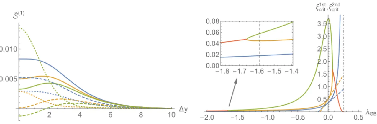
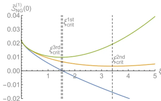
• Einstein gravity. The functions ˜a₄(˜u) and ˜b₄(˜u) are known up to third order in hy-drodynamics and are given in (B.12). With these functions at hand we can extract the numbers ˜a(k)₄ and ˜b(k)₄ and then use formula (4.33). Figure 2 (left) shows some representative curves for ˜S(1)_{≡ S}(1)_τ4/3

0 /w4∆x43 as a function of ∆y for various val-ues of ξ = τ₀−1w−3/2 = {0,0.15,0.3,0.45,0.6} depicted in blue, orange, green, red and purple, respectively. The solid lines correspond to third-order hydrodynamics; the dashed and dotted lines correspond to second- and first-order hydrodynamics, respectively. For ξ = 0.45 the dotted curve becomes negative for small ∆y, indicat-ing that first-order hydrodynamics is no longer valid. For ξ = 0.6 both the dotted and dashed curves are negative for small ∆y. This indicates that second-order hy-drodynamics is also invalid at this time. Finally, for all values of ξthat were plotted, the solid lines are always positive, so third-order hydrodynamics is valid for these values. However, if we keep on increasing ξ, the solid lines will become unphysical for small ∆y at some point. We observe the following behavior for any finite value of ξ (in the range of parameters that we plotted): the value of ˜S(1) _{increases up to} a maximum ˜Smax(1) > 0 and then decreases monotonically to zero as ∆y → ∞. This implies that the positivity of ˜S(1) _{at ∆y = 0 is enough to guarantee a good physical} behavior for any ∆y. In figure2(right) we show the behavior of ˜S(1)_{(0) as a function} of ξ for first-, second- and third-order hydrodynamics, depicted in blue, orange and green, respectively, and we indicate the times at which it becomes negative. From the ∆y→0 limit of the correlator (4.36) we obtain the critical times:

τ_crit1st = 2.828w−3/2, τ_crit2nd = 1.987w−3/2, τ_crit3rd = 1.503w−3/2. (4.37)

These bounds are stricter than the ones derived from the transverse correlator (4.18), and decrease at each order in hydrodynamics, as expected.

• α0-corrections. The functions ˜a₄(˜u) and ˜b₄(˜u) are known to linear order in γ =

α03_{ζ(3)/8 = λ}−3/2_ζ(3)L6_{/8 and up to second order in hydrodynamics, and are} given in (B.13). With these functions in hand, we can extract the numbers ˜a(k)₄

and ˜b(k)₄ and then use the formula (4.33). Figure 3 (left) shows some representa-tive curves for ˜S(1) _{≡ S}(1)_τ4/3

JHEP10(2017)110

2 4 6 8 10 Δy

-0.004 -0.002 0.002 0.004 0.006 0.008 ˜(1)

0.2 0.4 0.6 0.8ξ

-0.006 -0.004 -0.002 0.002 0.004 0.006 0.008

˜(1)(0)

ξ_crit1st ξ_crit2nd ξ_crit3rd

Figure 2. Left: plots for ˜S(1) _{≡ S}(1)_τ4/3

0 /w4∆x43 for various values of ξ = τ

−1

0 w−3/2 =

{0,0.15,0.3,0.45,0.6}depicted in blue, orange, green, red and purple, respectively. The solid lines correspond to third-order hydrodynamics; the dashed and dotted lines correspond to second- and first-order hydrodynamics, respectively. Right: plots for ˜S(1)_{(0) for first-, second- and third-order}

hydrodynamics, depicted in blue, orange and green, respectively. The dashed vertical lines corre-spond to the critical times at each order in hydrodynamics.

small ∆y, indicating that second-order hydrodynamics becomes invalid faster at fi-nite coupling. We observe the same behavior as in Einstein gravity, namely that the positivity of ˜S(1) _{at ∆y= 0 is enough to guarantee a good physical behavior for any} ∆y. In figure 3(right) we show the behavior of ˜S(1)_{(0) both for γ = 0 andγ = 10}−3 as a function of ξ for first- and second-order hydrodynamics, depicted in blue and orange, respectively, and we indicates the times at which it becomes negative. From the ∆y→0 limit of the correlator (4.36) we obtain the following critical times:

τ_crit1st(γ) = 2.828 + 474.115γ +O(γ2)

w−3/2, (4.38)

τ_crit2nd(γ) = 1.987 + 275.079γ +O(γ2)w−3/2. (4.39)

These bounds increase as we increase the value ofγ and are stricter than the ones de-rived from the transverse correlator (4.19). Based on this, we can conclude that finite coupling corrections indeed tend to reduce the regime of validity of hydrodynamics.

• λGB-corrections. The functions ˜a4(˜u) and ˜b4(˜u) are known non-perturvatively inλGB

and up to second order in hydrodynamics, and are given in (B.14). With these functions at hand we can extract the numbers ˜a(k)₄ and ˜b(k)₄ and then use the for-mula (4.33). For small and negative values of λGB we observe qualitatively the same

behavior as for the γ−corrections: the critical time below which first- and second-order hydrodynamics break down increases, which is the expected behavior for a theory that flows from strong to weak coupling. On the other hand, positive values of λGB behave in the opposite way, and thus appear unphysical for λGB interpreted

as a coupling constant. From the ∆y→0 limit of the correlator (4.36) we obtain the following critical times:

τ_crit1st(λGB) = 2.828−16.971λGB+O(λ2GB)

w−3/2, (4.40)

τ_crit2nd(λGB) = 1.987−14.876λGB+O(λ2GB)