in the Term Structure Using Linear Models and Artificial Neural Networks
by
Norman R. Swanson Department of Economics The Pennsylvania State University
University Park, PA
and Halbert White
Research Group for Econometric Analysis Department of Economics University of California, San Diego
February 1993 revised: October 1994
A Model Selection Approach to Assessing the Information in the Term Structure Using Linear Models and Artificial
Neural Networks
ABSTRACT
We take a model selection approach to the question of whether forward interest rates are useful in predicting future spot rates, using a variety of out-of-sample forecast-based model selection criteria: fore-cast mean squared error, forefore-cast direction accuracy, and forefore-cast-based trading system profitability. We also examine the usefulness of a class of novel prediction models called "artificial neural networks," and investigate the issue of appropriate window sizes for rolling-window-based prediction methods. Results indicate that the premium of the forward rate over the spot rate helps to predict the sign of future changes in the interest rate. Further, model selection based on an in-sample Schwarz Information Criterion (SIC) does not appear to be a reliable guide to out-of-sample performance, in the case of short-term interest rates. Thus, the in-sample SIC apparently fails to offer a convenient shortcut to true out-of-sample perfor-mance measures.
Keywords: Artificial Neural Networks; Forecasting; Term Structure; Interest Rates; Rolling Windows; Model Selection; Information Criteria.
1. INTRODUCTION AND OVERVIEW
An issue of continuing interest in the finance literature is the extent to which forward interest rates are useful as predictors of future spot rates. Fama’s (1984) work represents a milestone in examining this issue, providing evidence that forward rates do indeed contain information about future spot rates. Mish-kin (1988) refines and updates Fama’s analysis by conducting tests of the hypothesis that forward rates have predictive content using econometric techniques that properly take account of heteroskedasticity and serial correlation neglected by Fama, by using a somewhat more general method for obtaining interest rates from the term structure, and by making use of data available subsequent to Fama’s. Mishkin too finds evidence that forward rates help predict future spot rates.
In this paper, we examine this issue from a model selection perspective in order to shed some addi-tional light, rather than from a classical hypothesis testing perspective, as in Mishkin (1988). Specifically, we address the question, "Given an array of alternative models for forecasting future spot rates and appropriate forecasting-based model selection criteria, does the model selected by this procedure make use of forward rates?" If so, we have additional direct evidence of the usefulness of forward rates in predicting future spot rates. If not, we have direct evidence to the contrary. We consider not only linear models, as in Mishkin (1988), but also a class of flexible non-linear functional forms called artificial neural networks. The results reported below provide additional support for the hypothesis that forward rates are indeed use-ful, and suggest that the class of non-linear models which is considered may also prove useful for forecast-ing interest rates. More specifically, we find that the premium of the forward rate over the spot rate helps to predict the sign of future changes in the interest rate.
We adopt the model selection perspective as a complement to the more traditional hypothesis testing approach for a variety of reasons, while noting that the two methods are not completely dissimilar (for example, when in-sample model selection criteria are used). Our first reason is the fact that model selec-tion permits us to focus directly on the issue at hand: out-of-sample forecasting performance. Next is the advantage that the model selection approach does not require specification of a correct model for its valid application, as does the traditional hypothesis testing approach. Another desirable feature of the model selection approach is that if properly designed, the probability of selecting the truly best model approaches
one as the sample size increases, in contrast to the traditional practice of fixing a test size and rejecting the null hypothesis at that fixed size regardless of sample size, thus ensuring that Type I errors (wrongly reject-ing the null hypothesis) will always occur with non-vanishreject-ing probability, no matter how much data is available.
A limitation of the model selection approach is that it can sometimes be difficult to assess the Type I error associated with testing the implicit model selection hypothesis that two models under consideration truly perform equally well based on observed differences in realized model selection criteria. The pro-cedure we implement will have this defect; however, this is a defect of the same order as using a tradi-tional test whose size is known only asymptotically. In the model selection case, the size is also known only asymptotically, but it is known to be zero, a consequence of the fact that the truly best model is selected with probability approaching one, as discussed above. Nevertheless, the distinction between the model selection approach and the traditional hypothesis testing approach should not be overemphasized. For example, the comparison of two nested models using a sample-based complexity penalized likelihood criterion (such as the Schwarz Information Criterion - SIC) amounts to a likelihood ratio test with the significance level being determined by the penalty term associated with the information criterion.
A final conceptual motivation for using the model selection approach is that it can be used in con-junction with traditional hypothesis testing procedures. As recently discussed by Pötscher (1991), once a model is selected by a procedure that yields the truly best model with probability approaching one, then one can test hypotheses about the parameters of the truly best model in the usual way without adverse asymptotic consequences for the size of the test. Of course, if one does not impose the belief that the model selected is correctly specified, then one must be careful to appropriately interpret the hypothesis being tested - for example, that the role of forward rates in the best model among those tested is nil, rather than that forward rates do not aid whatsoever in forecasting future spot rates. Due to the statistical com-plexity of the relatively computationally simple procedures considered here, we shall not engage in such hypothesis testing exercises, but leave development of the necessary distributions to other work. The rea-sons for this statistical complexity will become apparent below. We mention this final motivation so that the reader does not carry away the impression that we are proposing a substitute for traditional hypothesis
testing. In fact we are proposing a logically prior complement for cases when the two methods cannot be equated to one another.
By adopting this model selection perspective, we believe that we contribute not only to the discus-sion of the usefulness of forward rates as a predictor of future spot rates, but also to the methodology of examining this and similar issues. One dimension of this contribution is that we consider a variety of model selection criteria, including the SIC, together with three out-of-sample criteria: forecast mean squared error, forecast direction accuracy, and forecast-based trading rule profitability. Contributions are also attempted in a number of other related interesting directions. Specifically, we examine the usefulness of a class of novel nonlinear prediction models called "artificial neural networks" (e.g. Kuan and White 1994), and we examine the issue of appropriate window sizes for rolling-window-based prediction methods.
The rest of the paper is organized as follows. Section 2 discusses the data, while Section 3 discusses the models considered in this study. Section 4 describes our estimation methods and the model selection criteria examined here. Section 5 discusses the results for statistical performance measures and Section 6 discusses the results for profitability performance measures. Section 7 contains a summary and concluding remarks.
2. THE DATA
We use data graciously provided by Frederic S. Mishkin, as used in his study (Mishkin 1988). Two objects are of interest: Rt +τ, the 1-month spot rate observed at time t + τ−1; and Fτ,t, the forward rate for month t+τobserved at time t. (This notation is similar to that in Fama (1984) and Mishkin (1988).) As described by Mishkin (1988, p. 309), end of month U.S. Treasury bill rate data were obtained from the Center for Research on Security Prices (CRSP) at the University of Chicago. The one-month bill is defined to have a maturity of 30.4 days, the two month bill 60.8 days, and so on, up to the six month bill with a maturity of 182.5 days. For each defined maturity the interest rate was interpolated linearly from the two bills that were closest to the defined maturity. As pointed out by an anonymous referee, it should be noted that the Mishkin data which is used here does not make use of actual transactions price data, as in
Fama (1984), since the interest rates are interpolated from the two bills that are closest to the defined rity. Thus, while the Mishkin data has the advantage that the term structure slope around the desired matu-rity is constant rather than zero and is thus less restrictive, using actual transactions price data is more suit-able when the focus is on predicting future premiums in the market. For this reason, the discussion of the most profitable regression model given a specific trading strategy (Section 6) should be thought of as methodological, and not as suggesting that the results will hold when dealing with actual prices in the market.
3. THE MODELS
3.1 Linear Models
Mishkin (1988) considers the following two models estimated by Fama:
Rt+τ− Rt +1 = α + β (Fτ,t−Rt +1) + νt +τ−1 (1) Rt+τ− Rt+τ−1 = α + β (Fτ,t−Fτ−1,t) + νt +τ−1 . (2) In these models, it is of interest to test whetherβ0, the "true" value ofβ, is zero. If so, the forward rate is unimportant (linearly) in predicting future spot rates. If not, forward rates contain useful predictive infor-mation. As Fama (1984) discusses, the null hypothesis (β0 = 0) occurs when risk premiums in forward rates obliterate the predictive relationship that would occur in the absence of these premiums. Fama (1976) and Shiller, Campbell and Schoenholtz (1983) find no evidence against the null, while Fama (1984) and Mishkin (1988) do find evidence against the null.
In this study, we consider these models as special cases of a fairly broad array of forecasting models. We refer to models with dependent variables Rt+τ− Rt +1as "Case 1" and models with dependent variables Rt +τ− Rt +τ−1as "Case 2."
For Case 1, we consider linear models containing the following regressors: a constant; lags of
Fτ,t− Rt +1from orders zero to two; and lags of Rt +τ− Rt +1 from "observable order" one to three. By a lag of "observable order" one, we mean the first lag of Rt +τ− Rt +1 observable at time t, i.e. Rt +1− Rt +1−τ, and so on for observable lag orders two and three. We separately consider models with a constant only, a con-stant and lags of Fτ,t− Rt +1, a constant and observable lags of Rt +τ− Rt +1, and a constant, lags of
Fτ,t− Rt +1 and observable lags of Rt +τ− Rt +1. The number of lags included was dictated by the necessity of keeping the total number of regressions to a manageable number, while still exploring a range of plausi-ble possibilities.
Table 1 provides a summary of the regressors included in the Case 1 regressions. The linear regres-sions are Models 1.0 through 1.16. Note that Model 1.0 is the simple random walk model (i.e. (1) withα andβ both constrained to zero), while Model 1.2 coincides with (1). The models differ primarily in the number of included lags. Table 1 also references two models (1.17 and 1.18) which we discuss below.
For Case 2, we consider linear models containing the following regressors: a constant; lags of
Fτ,t− Fτ−1,tfrom orders zero to two; and lags of Rt +τ− Rt +τ−1 from observable order one to three. As in Case 1, we consider separately models with a constant only, a constant and lags of Fτ,t− Fτ−1,t, a constant and observable lags of Rt +τ− Rt +τ−1, and a constant, lags of Fτ,t− Fτ−1,t and observable lags of Rt +τ− Rt +τ−1. Table 1 provides a summary of the regressors included in the Case 2 regressions, with linear regressions designated as Models 2.0 through 2.16. Also referenced are models 2.17 and 2.18, which are discussed below. Model 2.2 coincides with (2) above, while Model 2.0 is again the random walk (α = β = 0).
3.2 Nonlinear Models
Cognitive scientists have proposed a class of flexible nonlinear models inspired by certain features of the way that the brain processes information. (A good introduction to the cognitive science literature is Rumelhart and McClelland (1986).) Because of their biological inspiration, these models are referred to as "artificial neural network models" or simply "artificial neural networks" (ANNs). Because of their flexi-bility and simplicity, and because of demonstrated successes in a variety of empirical applications where linear models fail to perform well (see White (1989) and Kuan and White (1994) for some specifics), ANNs have become the focus of considerable attention as a possible vehicle for forecasting financial vari-ables. Among recent applications are those of White (1988), Dutta and Shekhar (1988), Moody and Utans (1991), Dorsey, Johnson and van Boening (1991), Dropsy (1992), and Kuan and Liu (1992). See also the recent book by Trippi and Turbau (1993).
For those interested in a detailed discussion of ANNs and their econometric applicability, we refer to Kuan and White (1994). For present purposes, it suffices to treat these models as a potentially interest-ing black box, deliverinterest-ing a specific class of nonlinear regression models. In particular, the ANN nonlinear regression models considered here have the form:
f(x, θ) = x˜´α + j =1
Σ
q
G(x˜´γj) βj (3)
where x˜ is a (column) vector of explanatory variables, x˜ = (1, x´)´ augments x by the inclusion of a con-stant term,θ = (α´, β´, γ´ )´,β = (β1, . . . ,βq)´,γ = (γ´, . . . ,γq´ )´, q is a given integer and G is a given non-linear function, in our case, the logistic cumulative distribution function (c.d.f.) G (z) = 1/(1 + exp(−z)).
A network interpretation of (3) is as follows. "Input units" send signals x0(= 1), x1, . . . ,xr over "connections" that amplify or attenuate the signals by a factor ("weight")γji, i =0, . . . , r, j =1, . . . , q. The signals arriving at "intermediate" or "hidden" units are first summed (resulting in x˜´γj) and then con-verted to a "hidden unit activation" G(x˜´γj) by the operation of the "hidden unit activation function" G. The next layer operates similarly, with hidden activations sent over connections to the "output unit." As before, signals are attenuated or amplified by weightsβjand summed. In addition, signals are sent directly from input to output over connections with weightsα. A nonlinear activation transformation at the output
is also possible, but we avoid it here for simplicity.
In network terminology, f (x, θ) is the "network output activation" of a "hidden layer feedforward network" with "inputs" x and "network weights"θ. The parameters γj are called "input to hidden unit weights," while the parametersβjare called "hidden to output unit weights." The parametersαare called "input to output unit weights."
Hornik, Stinchcombe and White (1989, 1990) (among others, see also Cybenko 1989, Carroll and Dickinson 1989 and Funahashi 1989) have shown that functions of the form (3) are capable of approximat-ing arbitrary functions of x arbitrarily well given q sufficiently large and a suitable choice of θ. This "universal approximation" property is one reason for the successful application of ANNs. In fact, White (1990) establishes that ANN models can be used to perform nonparametric regression, consistently estimating any unknown square integrable conditional expectation function.
Here we apply model (3) to the problem of forecasting Rt+τ− Rt +1 (Case 1) or Rt+τ− Rt +τ−1(Case 2) using explanatory variables x corresponding to all the variables considered in the linear forecasting models described above, and with q = 4. Note that whenβ1 = β2 = β3 = β4 = 0, we have Models 1.16 and 2.16 as a special case. Inclusion of the nonlinear terms G(x´ γj) should enhance forecasting ability, if overfitting is properly avoided.
These nonlinear artificial neural networks appear in Table 1 as Models 1.18 and 2.18. We also con-sider a final linear model, designated as Model 1.17 or 2.17, in which no hidden units are included, but for which the linear regressors are selected stepwise (with regressors added one at a time as in the ANN models - see Section 4). Due to constraints in the manner in which inputs can be specified for considera-tion in our software, it was necessary to permit a fourth observed lag of the dependent variable to be avail-able to the Models 1.17, 1.18, 2.17, and 2.18, for selection. In no case was the 4th lag selected, however, so that while the possible presence of this variable is indicated in Table 1, its inclusion in fact had no impact on the relative forecasting performance of our models.
The parameters of Models 1.0-1.16 and 2.0-2.16 are estimated by the method of least squares. How-ever, because of the possibility that the underlying relation between forward and future spot rates is evolv-ing through time, we estimate parameters usevolv-ing only a finite window of past data rather than all previously available data. Window sizes of 42, 60, 78 and 96 months are used for our regressions.
To evaluate the linear regression models and the various window widths, a sequence of out-of-sample one-step ahead forecast errors is generated by performing the regression over a given window ter-minating at observation T, say, and then computing the error in forecasting RT +τ+1 − RT +2 (Case 1) or RT +τ+1− RT +τ (Case 2) using data available at time T + 1 and the coefficients estimated using data in the window terminating at time T. Each time the window rolls forward one period, a new out-of-sample resi-dual is generated, simulating true out-of-sample predictions and prediction errors made in real-time by this process. For our study, the smallest value for T corresponds to February of 1979 and the largest to June of 1986. We therefore have a sequence of 89 out-of-sample one-step forecast errors with which to evaluate our models. This period was selected to cover the most recent Federal Reserve policy regimes observable in the data (occurring in October 1979 and October 1982), while still obtaining a computationally manage-able out-of-sample period.
By simulating forecasts in real-time, we obtain measures of forecasting performance analogous to those recently discussed by Diebold and Rudebusch (1991). Our procedure differs from theirs in that: (1) Diebold and Rudebusch (1991) use a growing data window with fixed first observation, as they are not concerned with tracking a possibly evolving system; and (2) Diebold and Rudebusch (1991) focus on the effects of using unrevised instead of revised leading indicators in real-time simulations, for predicting economic upturns and downturns. As we focus on financial market data which is accurately available in real-time, we have no need to worry about revision effects.
Four measures of out-of-sample model/window performance are computed in this paper. The first is the forecast mean squared error (FMSE) of the 89 one-step forecast errors for each model and window, and for each horizonτ = 2, . . . , 6. Using this measure, we can precisely address the question "Does the model/window combination with the smallest FMSE include the forward rate?" If so, we have direct and specific evidence of the value of forward rates in predicting future spot rates. The out-of-sample forecast
R2is also calculated, where
R2 = 1 − FMSE /S Y
2, (4)
and SY2 is the sample variance of the dependent variable in the out-of-sample period. Of note is that (4) can take negative values because the FMSE can exceed SY2, out-of-sample.
The second measure of forecast performance which is calculated is how well a given forecasting procedure identifies the direction of change in the spot rate, regardless of whether the value of the change is closely approximated. To examine this aspect of forecast performance, we calculate the "confusion matrix" of the model/window combination. A hypothetical confusion matrix is given as (5).
predicted down up H I 1236 26 15J K up down actual (5)
The columns in (5) correspond to actual spot rate moves, up or down, while the rows correspond to
predicted spot rate moves. In this way, the diagonal cells correspond to correct directional predictions,
while off-diagonal cells correspond to incorrect predictions. We measure overall performance in terms of the model’s "confusion rate," the sum of the off-diagonal elements, divided by the sum of all elements. As (5) is simply a 2×2 contingency table, the hypothesis that a given model/window combination is of no value in forecasting the direction of spot rate changes can be expressed as the hypothesis of independence between the actual and predicted directions. Methods for testing the independence hypothesis in the con-text of forecasting the direction of asset price movements have been given by Henriksson and Merton (HM, 1981). Based on the hypergeometric distribution, the p-values delivered by HM’s method require for their validity the independence of the directional forecast from the magnitude of the asset price change. We present the HM p-values. As with the FMSE, a finding that the least confused model contains the for-ward rate is direct evidence that forfor-ward rates are useful predictors of the direction of spot rate changes.
As a third measure of the relevance of forward rates in predicting future spot rates it is determined whether profitable trading strategies can be devised that make use of forward rate information. Although mean-variance values for the trading strategy are calculated, it should be noted that a relevant question is whether the investment is on the conditional mean-variance frontier at each point in time. Unfortunately,
resolving this question is beyond the scope of the present work. Because of the nature of the forecasts involved, the profitability analysis can be conducted only for Case 1 models. Further discussion of this performance measure is given in Section 6.
A drawback of the use of out-of-sample based model selection procedures is that they can be quite computationally intensive. Much less demanding procedures that use only in-sample information can be based on a variety of complexity-penalized likelihood measures. Among those most commonly used are the Akaike Information Criterion (AIC) (Akaike 1973, 1974) and the Schwarz Information Criterion (SIC) (Schwarz 1978, Sawa 1978). These information criteria add a complexity penalty to the usual sample log-likelihood, and the model that optimizes this penalized log-likelihood is preferred. Because the SIC delivers the most conservative models (i.e. least complex) and because the SIC has been found to perform well in selecting forecasting models in other contexts (for example, see Engle and Brown 1986), we exam-ine its behavior in the present context as a final measure of forecast performance. Two questions are of interest: First, taking the SIC at face value as a reasonable model selection criterion, does the SIC-selected model contain the forward rate? Second, what sort of guide is the in-sample SIC to out-of-sample performance? The first question is directed to our main issue of interest. The second question is of nearly equal importance, however, for if the relatively straightforward SIC reliably identifies the model that per-forms best according to one of our out-of-sample criteria, then we may use SIC as a welcome computa-tional shortcut.
For a model with p parameters estimated on a window of size n, the SIC is
SIC = log s2 + p(log n)/n , (6)
where s2is the regression mean-squared-error. The first term is a goodness of fit measure, and the second is the complexity penalty. We report the mean of the 89 values for the SIC, called MSIC, for given model/window combinations.
So far, no mention has been made of how the ANN models are estimated. It is to this issue that we now turn. In estimating the ANN models 1.18 and 2.18, it is inappropriate to simply fit the network param-eters with q = 4 hidden units by least squares, as the resulting network typically will have more paramparam-eters than observations, achieving a perfect or nearly perfect fit in sample, with disastrous performance
out-of-sample. To enforce a parsimonious fit, the ANN models were estimated by a process of forward stepwise (nonlinear) least squares regression, using the SIC to determine included regressors and the appropriate value for q. Specifically, a forward stepwise linear regression is performed first, with regressors added one at a time until no additional regressor can be added to improve the SIC. The linear regression coefficients are thereafter fixed. Next a single hidden unit is added (i.e. q is set to 1), and regressors are selected one by one for connection to the first hidden unit, until the SIC can no longer be improved. Then a second hid-den unit is added and the process repeated, until four hidhid-den units have been tried, or the SIC for q hidhid-den units exceeds that for q−1 hidden units. This ANN model selection procedure is begun anew each time the data window moves forward one period. A different set of regressors and a different number of hidden units connected to different inputs may therefore be chosen at each point in time. We thus simulate a fairly sophisticated real time ANN forecasting implementation. We should expect the ANN models to have SIC values superior to (i.e smaller than) those of the linear models, as the ANN model can choose any of the linear models as a special case.
Interestingly, even this fairly conservative procedure did not entirely eliminate the tendency for the neural network model to overfit, as evidenced by occasional totally wild one-step forecasts from network models that fit very nicely in sample. Accordingly, we impose a simple "insanity filter" on the network forecasts: if a one-step ahead predicted change exceeds the maximum change observed during the estima-tion window, then the forecast from Model 1.1 (or Model 2.1) - which includes only a constant - is used instead. Thus, we substitute ignorance for craziness. The performance of the ANN models and the linear forward stepwise regression models (Models 1.17 and 2.17) are evaluated in the same way as Models 1.0-1.16 and 2.0-2.16. For each we calculate the FMSE averaged over the 89 out-of-sample observations, the out-of-sample R2, the confusion matrix, confusion rate and HM p-values, and we perform a profitability analysis.
5. THE RESULTS FOR STATISTICAL PERFORMANCE MEASURES
To aid in the discussion of the results, a list of the acronyms used is given.
HM p−value FMSE MSIC SIC ANN
P−value for Henriksson−Merton test of the
Forecast Mean Squared Error: avg of 89 1−step forecasts Mean Schwarz Information Criterion
Schwarz Information Criterion: SIC = log s2 + p(log n)/n nonlinear model: arti ficial neural network
The results for Case 1 are summarized in Table 2, while those for Case 2 are in Table 3. In each case, a number of fairly clear-cut conclusions emerge. It should be noted that in both tables, statistical ties some-times occur. For the sake of brevity, though, this information has not been included, and the best models with the smallest window size, and fewest parameters are reported. More detailed results are available by request from the authors.
In Case 1, our main question of interest is answered affirmatively. For the period 3/79 through 7/86, the forward rate is valuable in predicting future spot rates, in that it appears in the model with the best FMSE for all but horizon τ = 6 and in the model exhibiting the least confusion, for all time horizons, τ = 2,..., 6. In fact, for the shortest horizon, τ = 2, the FMSE-best model is the simplest model including the forward-spot differential, Model 1.2 (corresponding to equation (1)), with maximum window size of 96 observations. For other horizons, more complex models are FMSE-best. Model 1.10, which adds three observable lags of the dependent variable to the simple Model 1.2 is FMSE-best at horizon τ = 3,4,5. However, atτ = 6, forward rates no longer enter the FMSE-best model (Model 1.5), which contains only a single observable lag of the dependent variable. A notable feature of our results is the fairly impressive out-of-sample R2’s obtained for each of the FMSE-best models. These range from a low of .062 forτ = 6 to a high of .142 forτ = 4. In each case, a window size of 96 observations is among the FMSE-best, but smaller window sizes also deliver identical performance for horizonsτ = 3 andτ = 4. In fact, forτ = 4 window sizes of 42, 60 and 96 deliver identical FMSE performance, suggestive of a mild degree of time instability.
Not surprisingly, the FMSE-best models are not generally the least confused (based on the HM p-value), as forecast errors for individual observations can simultaneously be small in magnitude and associ-ated with a prediction of the wrong sign. This is especially likely in prediction of small changes in spot rates. In all cases, the least confused model includes the forward-spot differential. Model 1.10 appears as least confused atτ = 2 andτ = 3, while Model 1.18 (the non-linear ANN model) appears as least confused at horizonsτ = 4 and 5. Model 1.3 is least confused forτ = 6. Model 1.13 matches the performance of Model 1.10 atτ = 2, while Model 1.16 matches the performance of Model 1.18 atτ = 5. In each case, the HM p-values are rather low, suggesting that correct directional prediction is not simply due to chance. In
fact, the least confused models are correctly predicting the direction of spot rate change approximately 2/3 of the time or better. The window widths for the least confused model are, in all but one case, smaller than the maximum size of 96. This is more strongly suggestive of time instability in the underlying process than the results for the FMSE. However, we cannot rule out the possibility that an estimation technique targeted directly on forecasting the direction of change (e.g., logit) would lead to out-of-sample confusion optimized by choosing the largest window sizes. We leave such analysis for future research.
As a final statistical performance measure, we consider the relation between the models identified as
best in Table 2 using the (in-sample) MSIC and those identified as best by the out-of-sample FMSE, or the
confusion criterion. As should be expected, the MSIC-best model is in each case the ANN model (Model 1.18), as these models are arrived at by minimizing the SIC in each window. However, in no case does the ANN model deliver best out-of-sample FMSE performance. Instead, the ANN model delivers least con-fused directional prediction at horizonsτ = 4 and 5. This is interesting, as it suggests that (at least in the present context) the MSIC cannot be used as a reliable shortcut to identifying models that will perform optimally out-of-sample. In network jargon, the MSIC-best model is not necessarily the model that "gen-eralizes" best when presented with data not included in the "training set". Instead, it is necessary to do the appropriate out-of-sample analysis to find the best model, when using non-linear artificial neural networks. Because of the combinatorial nature of this analysis for neural networks with hidden units, we defer this to subsequent work.
We note that the SIC is widely believed to select very parsimonious models, and that such models usually "win" forecasting competitions. Our results suggest that, at least in the present case, the SIC is not selecting sufficiently parsimonious models. As the SIC imposes the most severe penalty among the various alternatives (AIC, Hannan-Quinn, etc.), use of other such criteria would likely give worse-performing results. Out-of-sample analysis remains the only recourse.
Table 2 also provides summary statistics for models other than those deemed as best, using the per-formance measures. In particular, Table 2 contains results for Models 1.1 and 1.18, to provide background against which to compare the best models, and to provide additional insight into how well the least (Model 1.1) and most (Model 1.18) complex models perform. Recall that Model 1.1 contains only a constant term,
and so implements a random walk with drift. The R2’s for these models are effectively zero. However, for τ = 1, 2, 3, 4, 5 the nonlinear ANN model is no more confused than the best model (based on a p-value of 0.05). Thus, there is some evidence that the nonlinear models can help to predict the direction of change of the spot rate.
The results for the Case 2 regressions are less emphatic in their evidence for the value of the forward rate in predicting future changes in spot rates. For these regressions, the best FMSE at all horizons is achieved for the model containing only a constant (Model 2.1). (Note that only horizonsτ = 3, . . . , 6 are reported, as horizon τ = 2 coincides with Case 1.) For the confusion measures, forward rates do appear in the least confused models at three of the four horizons. The ANN model is the least confused model for τ = 3, with the least confusion achieved by differing models (Models 2.7, 2.3, 2.5 and 2.9) for other hor-izons. In all cases, the best confusion rates are worse than those seen in Case 1. Nevertheless, the least confused models achieve statistical significance at the 10% level or better according to the HM p-values, at all four horizons, with correct directional predictions approximately 60% of the time. Again, the SIC does not identify either the FMSE- or confusion-best model, out-of-sample. Note that for all horizons (except τ = 5), the SIC best neural network on average contains zero hidden units. In this sense, Model 2.17 dominates Model 2.18 in Case 2.
6. RESULTS FOR PROFITABILITY PERFORMANCE MEASURES
Let∆τt≡ Rt +τ− Rt +1 be the change in the spot rate (the dependent variable for the Case 1 regres-sions) and for a given model/window combination, let ∆ˆτT+1 denote the first out-of-sample predicted change in spot rates from a window terminating at time T. A forecast of the future spot rate is then given by
RˆT+1+τ = ∆ˆτT+1 + RT +2 (7)
A simple "straddle" or "spread" trading strategy can be based on (7). Specifically, sell the horizon τ forward instrument short if
RˆT+1+τ > τFτ,T +1− (τ−1)Fτ−1,T +1 , τ = 2, . . . , 6 . (8) With the proceeds from the short sale, buy theτ−1 horizon forward instrument, and when it matures use
the proceeds to purchase the spot instrument. If
RˆT+1+τ < τFτ,T +1− (τ−1)Fτ−1,T+1 , τ = 2, . . . , 6 , (9) undertake the reverse strategy. For simplicity we assume a standard contract of size $1 MM = $1,000,000. The profit (negative profit represents loss) for such a transaction is given by
Πτ,T +1≡ $1 MM(e
[τFτT +1−(τ−1) F(τ−1)T +1]−
e−RT +1+τ) − T
τ,T +1 , (10)
where Tτ,T +1is the total transactions cost associated with the spread. This cost includes both commissions and the effects of the bid-ask spreads. To avoid complexities associated with bid-ask spreads and with the effects of investor characteristics on commission costs, we consider a range of fixed values for Tτ,T +1, chosen to represent plausible possibilities for average total transactions costs. A simple measure of model/window performance is then given by the sum (undiscounted) of profits over the 89 out-of-sample observation periods.
Conditional on the realized history of asset prices, this profit measure is dependent on the particular realized pattern of correct directional predictions. This dependence can be removed under appropriate conditions by Monte Carlo simulation. To avoid having our conclusions adversely affected by dependence on a particular pattern of correct predictions, we report the results of a relevant Monte Carlo simulation. We follow an approach to trading-rule evaluation given by Leitch and Tanner (1991) and Dorfman and McIntosh (1992). The idea is that if a trading system gives a correct signal (i.e. one profitable apart from transactions costs) d × 100% of the time (0 ≤ d ≤ 1), and if correctness of a given signal is independent of correctness of prior signals and also independent of the magnitude of profit, then one can simulate the pro-bability distribution of trading system profits conditional on a realized price series of length n by repeat-edly drawing length n sequences of i.i.d. signals correct d × 100% of the time and computing the empiri-cal distribution of the resulting profits over a large number of replications.
In our case, our signals are "correct" if
(RˆT+τ+1 + (τ−1)Fτ−1,T +1−τFτ,T +1)(RT +τ+1 + (τ−1)Fτ−1,T +1−τFτ,T +1) > 0 . (11) The number of times this occurs divided by 89 gives our value for d. For each horizon, we identify the model/window combination giving the highest value for d. These are reported in Table 4. Generally, d is never less than 0.82, with d = 0.90 for τ = 2. This rather good performance was pleasantly surprising to
us. To investigate whether this performance is consistent with pure luck, we again compute the HM p-values associated with the confusion matrices. We reject the null hypothesis of independence in all cases rather decisively.
Of particular interest is the fact that in three of the five horizons, τ = 2, 3, and 5, forward rates or their lags enter the best model. This provides additional evidence of the value of forward rates in predict-ing future spot rates. We note that in no case does the d-best model correspond to the confusion best model for Rt +τ− Rt +1, and that there is no necessary correspondence. Also of interest is the fact that the d-best model forτ = 2 is the ANN model, with the highest observed value for d, and that the ANN is nearly d-best in all other cases (not shown in the table).
Next, we investigate whether signal correctness is independent of prior signal correctness. For this, we construct a sequence of Bernoulii random variables equal to 1 for a correct signal and 0 otherwise. We then perform a standard runs test (e.g., Mendenhall, Wackerly and Scheaffer 1990) on the observed sequence for the d-best model at each horizon. The null hypothesis of independence is decisively rejected for all horizons. These results are available from the authors, by request. Because lack of independence could presumably be used to improve a trading system, profit computations such as those reported here, which are based on independence, will be conservative.
As a final check on the relevance of the simulation framework, we investigated whether profit mag-nitude is independent of signal correctness by regressingA RˆT +1+τ + (τ−1)Fτ−1,T +1−τFτ,T +1A on a constant and a signal correctness dummy variable, DT +1. Under the null hypothesis of independence, the coefficient on the dummy variable should be zero. Marginally significant results appear at τ = 5 andτ = 6 with p-values of 0.045 and 0.06 respectively. Results otherwise are far from significance at conventional levels. These results are available, by request.
Thus, Dorfman and McIntosh’s (1992) simulation method for approximating the probability distribu-tion of trading system profits for a system correct d × 100% of the time should give some reasonably infor-mative benchmarks. Our results, reported in Table 5, are based on 10,000 replications. Results are reported for total transactions cost levels of from $0 to $1250, in increments of $250 per spread. Analysis of bid-ask spreads by Shen (1992) suggests that average costs of $250 may be realistic for large
institutional investors. Only the first moments are shown in Table 5. The simulated variances of the profits shown in the table are very small, in all cases below $20. As pointed out by an anonymous referee, it might also be useful to consider variances which are simulated by taking the average of the variance of profits for each of the 10,000 trials. In this case, the mean should also be the average of the average of each trial (i.e. the average profit per monthly transaction). Thus, since the experimental forecast horizon is 89 months long, the mean profit reported by us is 89 times as big as the mean profit which results from the suggested
alternative method for reporting the simulation results. In this case, however, the variances estimated are
still 3 orders of magnitude less than the mean. To illustrate the difference between the two methods for calculating the mean and variance of profits acruing from the trading strategy, (12) shows the mean and corresponding variance of profits which are reported here, while (13) does likewise for the alternative reporting strategy. With n=10,000 we have
mean(Π __ )1 = n 1 __ i =1
Σ
n H A Ij =1Σ
89 πi, jJA K , var(Π __ )1 = n 1 __ i =1Σ
n B A Di =1Σ
89 πi, j− HA I n 1 __ i =1Σ
n j =1Σ
89 πi, jJA K E A G 2 (12) mean(Π __ )2 = n 1 __ i =1Σ
n H A I 89 1 ___ j =1Σ
89 πi, jJA K , var(Π __ )2 = n 1 __ i =1Σ
n H A I 89 1 ___ i =1Σ
89B A Dπi, j− 89 1 ___ j =1Σ
89 πi, jEA G 2J A K (13)The story that emerges from the simulated profits reported in Table 5 is coherent and rather interest-ing. Positive profits occur at all horizons with total transactions costs per spread of up to $500, with posi-tive profits persisting to the $1250 level atτ = 5. The standard deviation of profit is quite small, relative to the typical magnitude of the average. While this suggests that potentially profitable information may be publicly available, and in particular in forward rates for horizons τ = 2, 3 and 5, the lack of a proper mean-variance frontier analysis and caution dictate that further detailed analysis should be carried out before the approach described here is used to trade debt instruments. Nevertheless, the rather good perfor-mance in predicting directions of rate movements could well be valuable to market makers and primary dealers.
7. SUMMARY AND CONCLUDING REMARKS
inves-tigate the extent to which forward interest rates are useful as predictors of future spot rates. We offer the following conclusions. First, for our out-of-sample period, the best Case 1 model contains forward rates in four out of five horizons, based on a forecast mean squared error performance measure, and five out of five horizons, when chosen using a confusion performance measure. The best models from a trading profitability standpoint contain the forward rate for three of the five horizons. Forward rates are thus use-ful in predicting future changes in spot rates, to this extent. Second, windows of observations of less than maximal size occasionally appear as forecast mean squared error-optimal, generally appear as confusion-optimal and often appear as d-best (providing the best trading rule signal), suggesting instability in the relationships of interest. Third, the in-sample Schwarz Information Criterion does not appear to be a reli-able guide to out-of-sample performance, so it fails to offer a convenient shortcut to true out-of-sample performance measures for selecting models, and for configuring nonlinear artificial neural network models. Finally, artificial neural network (ANN) models appear to be promising for use in this forecasting context, and further refinement and application of ANN methods is warranted.
The work reported here is merely a starting point. A wide variety of further questions present them-selves for subsequent research, both theoretical and empirical. On the theoretical side, it is of interest to establish the statistical properties of the model selection procedures followed here. Of particular interest is obtaining asymptotic distributions for a test that the true rolling-window root mean squared error of two models is equal based on the realized difference in forecast mean squared errors.
Interesting empirical projects include conducting a similar analysis using even larger windows; adding post-1986 data to the sample; extending the out-of-sample period in both directions; adding addi-tional interesting predictor variables; using robust regression methods and/or regression methods based on maximizing in-sample excess returns; using out-of-sample criteria to configure ANN models; and investi-gating the performance of alternatives to ANN models such as Multivariate Adaptive Regression Splines (Friedman 1988). All of these projects we leave to future work.
ACKNOWLEDGEMENTS
We are grateful to Frederic S. Mishkin for providing the data used here, and for discussions with Robert F. Engle, Scott Gilbert, Pu Shen and Ross M. Starr. Financial support was provided by Social
Sciences and Humanities Research Council of Canada Award No. 753-91-0416 and by NSF Grants SES-8921382 and SES-9209023. Any errors are solely our responsibility.
Table 1: Included Regressors for Case 1 and 2 Regressions
1 Case 1: Rt +τ−Rt +1 = a1 + iΣ
α1,i(Fτ,t−i−Rt +1−i) + iΣ
β1,i(Rt +τ−i−Rt +1−i) + u1,t Case 2: Rt +τ−Rt +τ−1 = a2 + iΣ
α2,i(Fτ,t−i−Fτ−1,t−i) + iΣ
β2,i(Rt +τ−i−Rt +τ−1−i) + u2,t _________________________________________________________________ _________________________________________________________________Number of Lags Included, p
Hidden
Dependent
Exogenous
Units
Model #
0
1
2
1
2
3
4
_________________________________________________________________c. 0
c. 1
c. 2
x
c. 3
x
x
c. 4
x
x
x
c. 5
x
c. 6
x
x
c. 7
x
x
x
c. 8
x
x
c. 9
x
x
x
c. 10
x
x
x
x
c. 11
x
x
x
c. 12
x
x
x
x
c. 13
x
x
x
x
x
c. 14
x
x
x
x
c. 15
x
x
x
x
x
c. 16
x
x
x
x
x
x
c. 17
x
x
x
x
x
x
x
c. 18
x
x
x
x
x
x
x
x
_________________________________________________________________1The c in Model # corresponds to Case 1 and Case 2, so that Model 1.0 is model 0 for Case 1, and Model 2.0 is model 0 for Case 2, for example. For Cases 1 and 2, the dependent variables are Rt +τ−Rt +1 and Rt +τ−Rt +τ−1respectively. The exogenous variables are lags of Fτ,t−Rt +1and Fτ,t−Fτ−1,t respectively. For models 1.18 and 2.18, up to 4 hidden unit are included as regressors. All regressions include an intercept, except for Models 1.0 and 2.0.
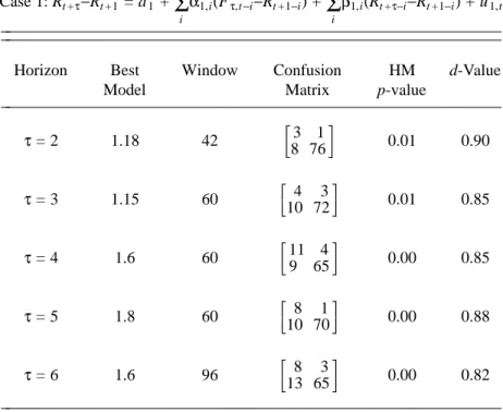
Table 4: Best d
−
Value Model by Window and Horizon
1 Case 1: Rt +τ−Rt +1 = a1 + iΣ
α1,i(Fτ,t−i−Rt +1−i) + iΣ
β1,i(Rt +τ−i−Rt +1−i) + u1,t ________________________________________________________ ________________________________________________________Horizon Best Window Confusion HM d-Value
Model Matrix p-value
________________________________________________________ τ = 2 1.18 42 HI 83 761JK 0.01 0.90 τ = 3 1.15 60 HI 104 72 3J K 0.01 0.85 τ = 4 1.6 60 HI 911 65 4J K 0.00 0.85 τ = 5 1.8 60 HI 108 701JK 0.00 0.88 τ = 6 1.6 96 HI 138 65 3J K 0.00 0.82 ________________________________________________________ 1
Models 1.18, 1.15, and 1.8 contain the current and/or lagged forward rate. The matrices shown in square brackets are confusion matrices (diagonal cells correspond to correct directional predictions, while off-diagonal cells correspond to
incorrect predictions). The d-Values are based on the number of times that
(RˆT+τ+1 + (τ−1)Fτ−1,T +1−τFτ,T +1)(RT +τ+1 + (τ−1)Fτ−1,T +1−τFτ,T +1) > 0 , divided by the out-of-sample size, 89. Thus, the trading system gives a correct signal (one profitable apart from transactions costs) dx100 percent of the time. The HM (Henriksson and Merton (1981)) p-values are based on the null hypothesis that a given model is of no value in predicting the direction of spot interest rate changes.
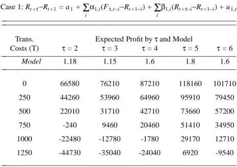
Table 5: Mean Profit Analysis by Horizon
−
in Dollars
1 Case 1: Rt +τ−Rt +1 = a1 + iΣ
α1,i(Fτ,t−i−Rt +1−i) + iΣ
β1,i(Rt +τ−i−Rt +1−i) + u1,t ________________________________________________________ ________________________________________________________Trans. Expected Profit byτand Model
Costs (T) τ = 2 τ = 3 τ = 4 τ = 5 τ = 6 ________________________________________________________ Model 1.18 1.15 1.6 1.8 1.6 ________________________________________________________ 0 66580 76210 87210 118160 101710 250 44260 53960 64960 95910 79450 500 22010 31710 42710 73660 57200 750 -240 9460 20460 51410 34950 1000 -22480 -12780 -1780 29170 12710 1250 -44730 -35040 -24040 6920 -9540 ________________________________________________________
1Best Models are chosen by d-Value, as listed in Table 4. The trading strategy entails risk, so no arbitrage is detected, and a proper financial evaluation entails consideration of not only mean profit (or return), but also risk, which is not considered here. The trading strategy assumes a standard contract of size $1MM, and follows equations (7)-(10), where the profit for a single transaction is given by: Πτ,T +1≡ $1MM(e
[τFτ,T +1− (τ−1)Fτ−1,T +1]
− e−RT+1+τ) − T
τ,T +1, where
Tτ,T +1 is the total transactions cost associated with the spread and is fixed at T in the simulations. Numerical values are based on 10000 simulations.
REFERENCES
Akaike, H. (1973), "Information Theory and an Extension of the Maximum Likelihood Princi-ple," in B. N. Petrov and F. Csaki, eds., 2nd International Symposium on Information Theory, Budapest: Akademiai Kiado, pp. 267-281.
__________ (1974), "A New Look at the Statistical Model Identification," IEEE Transactions on
Automatic Control, AC-19, pp. 716-23.
Carroll, S.M. and Dickinson, B.W. (1989), "Construction of Neural Nets Using the Radon Transform," in Proceedings of the International Joint Conference on Neural Networks, Washing-ton DC. New York: IEEE Press, pp. 607-611.
Cybenko, G. (1989), "Approximation by Superpositions of a Sigmoid Function," Mathematics of
Control Signals and Systems, 2, pp. 303-14.
Diebold, F.X. and Rudebusch, G.D. (1991), "Forecasting Output With the Composite Leading Index: A Real Time Analysis," Journal of the American Statistical Association, pp. 603-10. Dorfman, J.H. and McIntosh, C.S. (1992), "Using Economic Criteria for Forecast Valuation and Evaluation," mimeo, University of Georgia, February 1992.
Dorsey, R.E., Johnson, J.D. and van Boening, M.V. (1994), "The Use of Artificial Neural Net-works for Estimation of Decision Surfaces in First Price Sealed Bid Auctions," in W.W. Cooper and A. Whinston eds., New Directions in Computational Economics. Boston: Kluwer, pp. 19-40. Dropsy, V. (1992), "Exchange Rates and Neural Networks," California State University Fullerton Department of Economics Working Paper 1-92.
Dutta, S. and Shekhar, S. (1989), "Bond Rating: A Non-Conservative Application of Neural Net-works," in Proceedings of the IEEE International Conference on Neural Networks, San Diego. New York: IEEE Press, pp. 443-450.
Engle, R.F. and Brown, S.J. (1986), "Model Selection for Forecasting," Applied Mathematics and
Computation, 20.
Fama, E.F. (1976), "Forward Rates as Predictors of Future Spot Rates," Journal of Financial
Economics, 3, pp. 361-377.
__________ (1984), "The Information in the Term Structure," Journal of Financial Economics, 13, pp. 509-28.
Friedman, J. (1988), "Fitting Functions to Noisy Data in High Dimensions", in E.J. Wegman, D.T. Gantz and J.J. Miller eds., Computing Science and Statistics: Proceedings of the Twentieth
Sym-posium on the Interface. Alexandria VA: American Statistical Association, pp. 13-43.
Funahashi, K. (1989), "On the Approximate Realization of Continuous Mappings by Neural Net-works," Neural Networks, 2, pp. 183-92.
Henriksson, R.D. and Merton, R.C. (1981), "On Market Timing and Investment Performance. II. Statistical Procedures for Evaluating Forecasting Skills," Journal of Business, 54, pp. 513-33.
Hornik, K., Stinchcombe, M. and White, H. (1989), "Multilayer Feedforward Networks are Universal Approximators," Neural Networks, 2, pp. 359-66.
__________, __________ and __________ (1990), "Universal Approximation of an Unknown Mapping and its Derivatives Using Multilayer Feedforward Networks," Neural Networks, 3, pp. 551-60.
Kuan, C.-M. and Liu, T. (1992), "Forecasting Exchange Rates Using Feedforward and Recurrent Neural Networks," University of Illinois at Urbana-Champaign Bureau of Economic and Busi-ness Research Faculty Working Paper 92-0128.
Kuan, C.-M. and White, H. (1994), "Artificial Neural Networks: An Econometric Perspective,"
Econometric Reviews, 13, pp. 1-91.
Leitch, G. and Tanner, J.E. (1991), "Economic Forecast Evaluation: Profits Versus the Conven-tional Error Measures," American Economic Review, 81, pp. 580-90.
Mendenhall, W., Wackerly, D. D. and Scheaffer, R. L. (1990), Mathematical Statistics with
Applications, Boston: PWS-Kent.
Mishkin, F.S. (1988), "The Information in the Term Structure: Some Further Results," Journal of
Applied Econometrics, 3, pp. 307-14.
Moody, J. and Utans, J. (1991), "Principled Architecture Selection for Neural Networks: Appli-cations to Corporate Bond Rating Predictions," in J.E. Moody, S.J. Hanson and R.P. Lippmann, eds., Advances in Neural Information Processing Systems 4. San Mateo: Morgan Kaufman, pp. 683-690.
Pötscher, B.M. (1991), "Effects of Model Selection on Inference," Econometric Theory, 7, pp. 163-185.
Rumelhart, D. E. and McClelland, J. L. (1986), Parallel Distributed Processing: Explorations in
the Microstructures of Cognition, Cambridge: MIT Press.
Sawa, T. (1978), "Information Criteria for Discriminating Among Alternative Regression Models," Econometrica, 46, pp. 1273-92.
Schwarz, G. (1978), "Estimating the Dimension of a Model," The Annals of Statistics, 6, pp. 461-4.
Shen, P. (1992), "Determination of Bid-Ask Spreads in the Government Security Market: Theory and Empirical Tests," dissertation, University of California, San Diego, 1992.
Shiller, R.J., Campbell, J.Y. and Schoenholtz, K.L. (1983), "Forward Rates and Future Policy: Interpreting the Term Structure of Interest Rates," Brookings Papers on Economic Activity, 1, pp. 173-217.
Trippi, R. and Turbau, E. (1993), Neural Networks in Finance and Investing. Chicago: Probus Publishing Company.
White, H. (1988), "Economic Prediction Using Neural Networks: The Case of IBM Daily Stock Returns," in Proceedings of the IEEE International Conference on Neural Networks, San Diego. New York: IEEE Press, pp. 451-458.
__________ (1989), "Learning in Artificial Neural Networks: A Statistical Perspective," Neural
Computation, 1, pp. 425-64.
__________ (1990), "Connectionist Nonparametric Regression: Multilayer Feedforward Net-works Can Learn Arbitrary Mappings," Neural NetNet-works, 3, pp. 535-49.