Application of Genetic Algorithm to Maximise
Clean Energy usage for Data Centres
Raymond Carroll
Sasitharan Balasubramaniam
William Donnelly
Dmitri Botvich
TSSG, Waterford Institiute of Technology, Ireland (rcarroll, sasib, dbotvich, wdonnelly)@tssg.org
Abstract: The ICT industry is quickly becoming a very significant
consumer of global energy. This energy usage clearly comes at an environmental cost, and recent reports estimate that the industry
now contributes 2% of the worlds CO2 emissions, or as much as
the aviation industry. A significant part of this energy consumption can be attributed to data-centres, where huge numbers of energy-intensive servers host a variety of internet services. Much of this energy consumption is driven by the popularity of the Internet, which continues to attract growing numbers of users who now rely on the Internet as part of their daily lives. A major factor behind this attraction is the multitude of services available on the Internet, ranging from web based services (e.g. facebook) to heavy power consuming services such as multimedia (e.g. youtube, IPTV). As a result of this increased energy usage, the research community has become focused on finding solutions to improve the energy efficiency and carbon footprint of data centres. In this paper we present our solution for delivering green data centres. We propose a Genetic Algorithm-based solution for determining the optimal placement of services in data-centre network, in order to maximize the overall renewable energy usage and minimize the cooling energy consumption. We then perform a series of experiments in order to evaluate our solution, incorporating varying service request profiles and actual weather and renewable energy production values.
Keywords:Green Data Centres, Energy Efficiency, Genetic Algorithm
1 Introduction
It is now clear that the much debated predictions of increased climate change as a result of human activities are accurate. While it has been hotly disputed in the past, scientists now appear to be approaching consensus as climate change begins to have a real and visible effect. One of the most significant contributing factors is the increased levels of CO2 emitted into the atmosphere, which can be
largely attributed to human activity in the form of fossil fuel combustion. CO2, as
the most significant of the green house gasses, is contributing to global warming and ultimately rising sea levels and more extreme weather conditions. While it is developed countries that are the major producers of CO2 emissions, emerging
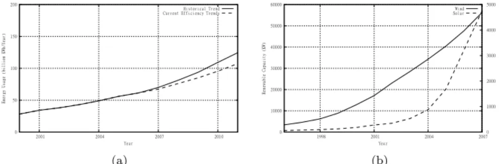
nations, such as China and developing 3rd world countries have the potential to exacerbate these trends enormously. As a result of this, in recent years, there has been an enormous push towards making all aspects of human activity more environmentally friendly. Indeed in the ICT industry there has been there has been a growing focus on the impact of the internet, and more specifically data-centres, on the environment, in terms of their increasing energy usage. Figure 1(a) shows that from 2000-2006 the energy usage of data centres in the US (EnergyStar, 2007) more than doubled. It also depicts the predicted trends up to 2010, extrapolated based on both the historical data and also based on recent trends towards energy efficiency, where both show huge increases in energy usage.
While these trends do consider the impact of the move towards more energy efficient practices, they do not consider the impact that new technologies and computing models may have. For instance the growth in the usage of smart phones in recent years has been exceptional. These phones are in essence resource limited computing platforms, where often times much of the processing is done in back-end service/application residing on the data-centre. Also, the recent move towards cloud computing holds huge potential for increasing data centre usage. Cloud computing proposes to move the majority of the application processing and data storage into the data centre, with thin client devices running simple interfaces. These emerging trends suggest that data-centres could grow beyond what has been predicted, and continue this rate of growth into the future. At the same time, many countries are now actively pursuing more renewable sources of energy, through their own capital infrastructure projects or through grid feed-in tariff incentive schemes. This is illustrated in Figure 1(b), where we show the recent capacity increases in wind and solar energy within the EU states (Eurostat).
Based on these developments, our work attempts to address the problem of data-centre energy usage by allowing data-centre operators to determine a service placement strategy with the best renewable and cooling energy profile. This in turn reduces the overall carbon footprint of the data centre operator. To do this we employ a genetic algorithm (GA) based service placement approach, where the GA determines the most optimal service/centres pairings to maximize data-centre usage of renewable energy sources and minimise cooling energy.
2 Related Work
There is now a considerable volume of research being carried out in the area of energy efficiency for data centres. Many have focused on consolidating workloads on a minimum number of servers in order to allow servers to be switched off/sleep to save power (Bradley et al, 2003) (Das et al, 2008) (Meisner et al, 2009) (Rusu et al, 2006). Barbagallo et al (2010) used biological mechanisms are used to determine more efficient servers in a data centre where load is subsequently moved. Others investigated how to make the data centres more efficient through better thermal management of the heat load on the cooling systems within a data centre. This is done by examining workload distribution and scheduling schemes to reduce the
0 50 100 150 200 2001 2004 2007 2010 En erg y Usa ge (bi ll io n KWh /Y ear ) Year Historical Trend Current Efficiency Trends
(a) 0 10000 20000 30000 40000 50000 60000 1998 2001 2004 2007 0 1000 2000 3000 4000 5000 Re new ab le Cap aci ty ( KW) Year Wind Solar (b)
Figure 1 (a) Data Centre Energy Trends, (b) Wind & Solar Capacity of EU countries
energy requirements of the cooling system (Bash and Forman, 2007) (Wang et al, 2009) (Sharma et al, 2005) (Moore et al, 2005) (Tang et al, 2008). (Patel et al, 2003) investigates moving load between countries based on the diurnal temperature and its impact on cooling, but does not consider renewable energy, uses a simple objective function to determine the best location and performs no significant evaluation. Garg et al (2010) take a similar approach to ours, where HPC applications are scheduled based primarily on the data-centres carbon emission rate, but do not employ a GA-based approach. Also, in (Qureshi and Weber, 2009) traffic load is moved between data centres based on electricity costs. Here sustainability of the data centres is not considered at all, meaning possible energy savings would be sacrificed in favour of cost savings.
3 Sustainable Energy Prioritization Solution
In previous work (Balasubramaniam et al, 2009) we used biological mechanisms such as replication and migration to perform a host of service management functions. In this paper our aim is to develop a solution, using GA, to drive the migration of services to data centres in such a way as to maximise renewable energy usage and minimise cooling energy. Specifically the GA is used to determine the best data-centre location (or placement) for each service, where this placement is based on two core factors. First is the level of renewable energy available at each data-centre, where data-centres with higher levels of renewable energy are clearly more desirable. Second is the cooling energy that is estimated to be required by the cooling systems in each data-centre, where data-centres with conditions more amenable to cooling are again preferred.
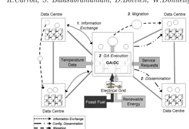
In this section we describe our approach, which is made up of two parts: a process for coordinating data-centres to share information and execute the new placement solutions (Section 3.1); and a genetic algorithm for determining the best service placement solutions (Section 3.3). While the GA determines the optimal solution, in order to do so it requires a complete picture of the state of all data-centres in the data-centre network. Specifically, it must be aware of the renewable energy consumption, the cooling efficiency and service load of each data-centre. The renewable energy is measured through a value we call the renewable energy ratio (RER - Section 3.4). Also, both the renewable energy and cooling energy
Figure 2 Service Placement Process
calculations are subject to the current load on the services in the data-centre, since higher loads expend more energy and generate more heat. In terms of cooling, the ambient temperature of the country can have a significant effect on the efficiency of the cooling system. This efficiency is measured through a value termed the Coefficient of Performance (COP - Section 3.4).
3.1 Service Placement Algorithm
In this section we describe the overall service placement process, including the steps that must take place before and after the GA determines the best placement solution. In Figure 2 we depict this process, which takes place in effectively three stages:
1. Information Exchange: Each data-centre has renewable energy, temperature and service load information available. Initially, all data centres must co-ordinate and share this information, as it forms the basis for our genetic algorithm in determining the fittest service configuration. In our solution the genetic algorithm is run periodically by a specific, pre-selected data centre (referred to as the GA-DC). However, for the purposes of redundancy each data centre is capable of running the algorithm and so the energy data is shared among all data centres.
2. GA Execution & Configuration Dissemination: As mentioned earlier, the genetic algorithm will determine the most optimal service/data centre configuration, based on maximising the usage of renewable energy and minimising the consumption of energy in cooling the data centre. The genetic algorithm is described in detail in the following sections. Once the optimal configuration has been found, this configuration is then disseminated to all data centres. Each data centre then examines this configuration and implements its recommendations.
3. Service Migration: To execute the GA-derived solution, the data centre determines which of its currently hosted services have been selected to move
Monitor Parameters
(Traffic, Renewable) Forecast Calculate Flucuation fl fl > threshold Execute GA Yes No
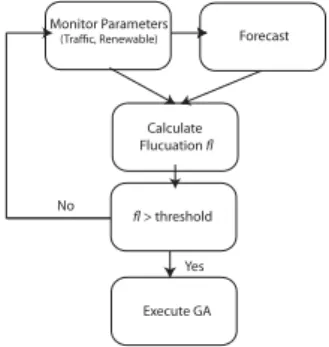
Figure 3 Dynamic Triggering
and to what data centre. Once ascertained, the data centres then migrate the selected services to their newly designated data centre. Each data centre is notified of the change in order to update their information registries and so that requests for the service at the originating data centre will be forwarded to its new location.
3.2 Dynamic GA Triggering
While our aim is to use GA to guide the migration of services to locations that will result in maximum renewable and efficient energy usage, there is clearly an overhead involved when potentially large groups of services move. To reduce this overhead it is desirable for the GA to run as infrequently as possible, while still maximizing the renewable energy and cooling energy savings. In this paper we will also look at dynamically invoking the GA based on monitoring of a number of important factors. These factors include the current service load and the current renewable energy ratios for each data-centre. Unless there has been a significant change in some of the contributing GA parameters then the GA is not required to run. To determine fluctuation we attempt to forecast both traffic and renewable energy values for the coming time period and then retrospectively compare the actual values to the forecasts. In (1) we show our general function for forecasting, based on Exponential Smoothing, where ot−1 represents the monitored value and
ρt−1 represents the previously predicted value (λis termed the Smoothing Factor,
allowing biasing towards monitored or predicted values). Since the forecast values are based on the observed values to date, these will be reasonably accurate when the data is smooth, and less accurate when there are fluctuations. Therefore, in order to determine fluctuations we then compare the previously predicted value to the actual monitored value. If the difference is greater than a certain threshold we deem this to be enough variation to warrant executing the GA. The process is shown in Figure 3. In order to reduce the possibility of highly localized spikes in either the request or energy rate, causing the GA to be mistakenly invoked, we use a sampling window of seven days. This means that each rate (traffic and RER) is monitored over the previous seven days and an average taken.
Figure 4 GA Problem Representation
3.3 Genetic Algorithm
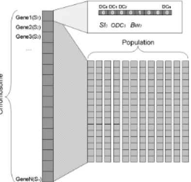
In implementing a GA we must first encode our problem solutions into a chromosome representation. In our algorithm each chromosome must represent a configuration of all services placed across the nine selected data centres. Our problem formulation is depicted in Figure 4, where each gene represents a single service placed on a single data centre. Specifically, each gene contains details of each service and an ordered list of binary values indicating the data centre on which the service is placed. Thus each chromosome is only as long as the number of services in the system.
When creating our initial population, we construct the chromosomes as represented in Figure 4. The GA then randomly selects a gene (service) from each chromosome and then randomly assigns this to a data-centre, subject to certain constraints which are discussed in Section 3.4 (e.g. available data-centre capacity). Once the initial population has been generated, we then calculate the fitness of each chromosome. We first calculate the fitness of each individual gene, by examining the workload details of the service, and the details of the data centre on which it is placed. Once each genes fitness has been calculated we can then sum these values to determine the overall chromosome fitness.
Using this fitness value we employ elitism, where the two fittest chromosomes are selected to be carried forward to the next generation. In order to populate the remainder of the new generation, we select two parent chromosomes using roulette wheel selection. We then perform single point crossover to generate new offspring chromosomes, where care is taken to ensure that the resulting chromosome(s) do not cause any data-centre to exceed its maximum capacity. Mutation is carried out by randomly changing the binary value indicating where a service is located data. This results in a new service allocation, where again care is taken to not break the constraints outlined later.
3.4 GA Fitness Function
Our fitness function is designed to measure the strength of a solution based on the renewable energy and cooling energy it is estimated to consume. Specifically,
the aim is to maximise the renewable energy consumed and minimise the cooling energy used. These are conflicting optimization goals, since the data centres with the best renewable energy ratio are not necessarily the data centres with the best environmental conditions for efficient cooling. The fitness function is presented in (2) below. Let the set of services be Si = s1, s2,...si...sN, where N is the total
number of services; the set of Data Centres be DCj=DC1, DC2,....DCj...DCM,
where M is the total number of Data Centres. Let RERj be the Renewable Energy
Ratio of data centre j, CEj be the Cooling Energy of Data Centre j, slij be the
service load of service i on data centre j, and DCCj is the capacity of data centre
j. α is a weighting parameter which allows us to prioritise the maximisation of renewable energy or the minimisation of cooling energy.
max M X j=1 N X i=1 ((1−α)(sli.RERDCj) +α 1 CEj ) (2) Subject to N X i=1 slij< DCCj (3)
To determine the renewable energy consumed we use the renewable energy ratio (RERj) of the data centre in question. The RER is the ratio of renewable energy
production to total energy production in the data centres host country (see also Section 4.1). This ratio gives us the best indication possible of what proportion of energy from renewable sources the data centre is consuming. However the quantity of renewable energy consumed is a factor of the load on the data centre also. As such we need to calculate the load exerted on the data centres by the service (sli).
The cooling energy (CE) of a data centre is calculated based on heat load (HL) to be removed from the data centre subject to the efficiency of the cooling system (COP) in removing this heat (see (4)). The heat load is directly related to the energy being consumed by the computing equipment, which is then converted to heat. As such we calculate the heat load by determining the power being used in the data centre. This is shown in (5) , wherePmax is the maximum power a single
server consumes at peak load,Pidleis the power a single server consumes while idle
(load = 0), sl is the load exerted on the server by a single service i and ns is the number of servers in the data centre. Since the idle power is consumed irrespective of server workload, the workload only impacts the power consumed above the idle power (Pmax−Pidle).
CE= HL COP (4) HL= N X i=1
(sli).(ns.(Pmax−Pidle)) +ns.Pidle (5)
Before we discuss the COP in more detail, there are constraints on the GA which we must mention. The utilisation of the services assigned to a specific data
centre cannot exceed the capacity of that data centre (3). In addition, a service must be assigned to only one data centre (especially important in crossover and mutation).
Coefficient of Performance (COP)
Critical to the calculation of the cooling energy fitness value is the Coefficient of Performance (COP) of each data centre. The COP value indicates the efficiency of the cooling system in removing the heat load from the data centre (6). A high COP means the thermodynamic process is more efficient.
COP = HeatLoad CoolingEnergy (6) COP = T 1 h Tc −1 (7)
Under the principles of thermodynamics (Moran and Shapiro, 1995), the efficiency of a typical heat pump is highly dependant on both the inside (target) temperature and the environmental (outside) temperature to which the removed heat is rejected. In (7) we can see that the greater the outside temperature (Th) is
(for a set inside temperature (Tc)) the more inefficient the system. In most cases,
once the outside temperature drops below the indoor temperature air conditioning is typically not required. However in the case of data-centres, the primary heat load is not coming from heat transfer from the environment but rather the computing equipment, so cooling is still required. In line with best practices of data centre cooling, we design each data-centre with a free cooling system in addition to conventional cooling. Free cooling allows data-centres to utilize the outdoor environmental conditions to part, or even fully, cool the data centres when conditions allow. Typically this is when the outside temperature is below the indoor temperature, thus free cooling is also highly dependant on the weather conditions. As a result we employ a COP model based on the assumption that both free-cooling and standard electric cooling are employed. Once the outdoor temperature is above the required cooling temperature, we use COP values based on standard electrical cooling. However, when the outdoor temperature drops below the required indoor temperature we move to free cooling and adapt the COP model inline with the changeover.
In this work we assume that standard cooling is provided by a generic heat pump as modelled by the Oak Ridge National Laboratory (ORNL) heat pump simulator. As such we take our standard cooling COP values from the ORNL simulator. We do not subscribe to a specific free-cooling system, instead we generalize based on the assumption that free-cooling provides a significant improvement in the efficiency of the cooling system. Thus for free cooling we simply adapt the values of the ORNL COP such that when the outside temperature drops below the inside temperature, we adjust the COP relative to the original COP value (e.g. +40%). This aims to represent that, once the outside temperature is cooler than inside, the free-cooling system is in operation. However we do not assume that free-cooling COP is uniform, as the energy required by a free-cooling system can vary depending on the extent by which the outside temperature is cooler than inside. For instance air-pumps may need to pump less
Population Size 100 Mutation Rate .02 Crossover Rate .7 Parameter Value No. Generations 60 Free-Cooling Efficiency 40% α 0.5
Table 1 Simulation Parameters
air to cool the server room the cooler the outside temperature gets. So, using this model we can determine the COP based on the known outside and inside temperature.
3.5 GA Evaluation
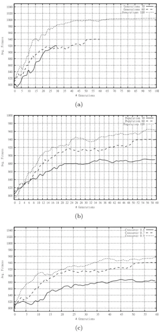
In this section we perform some initial evaluations of the genetic algorithm itself, to ensure its correct operation. We vary the main GA parameters (population size, generations, crossover rate) as seen in the results presented in Figure 5.
We start by varying the number of generations for which the GA runs, as seen in Figure 5(a). As expected the greater the number of generations the better the overall result. The smaller generation size does obtain a reasonable fitness value quickly, but the 60 and 100 generation simulations are able to obtain higher values over time. Increasing the population size reduces the effects of randomness and gives a more diverse starting population. As expected, Figure 5(b) demonstrates that this leads to a stronger average population fitness, increasing in line with the population size increase. Finally, again as we would predict, the higher crossover rates in Figure 5(c) lead to more diversity in the populations and hence allow fitter, more optimal solutions to be found. At a low crossover rate we can see that the algorithm struggles to improve the population fitness since it is more difficult to breed new solutions from parents with higher fitness values.
4 Simulation and Results
In the following section we perform a case study simulation of the potential renewable energy gains possible for a small sized data centre operator, based on the genetic algorithm and scenario outlined in the following sections. Our simulations are presented in two sets. Set A evaluates the systems performance over an extended period of time with a flat traffic rate and a fixed GA-execution schedule (monthly). The second set (B) is aimed at evaluating the ability of the system to dynamically detect changes in the network and trigger the GA to re-configure the service placements. This simulation examines the performance over a slightly shorter time-period with a fluctuating traffic profile, where we also sample the traffic at a finer time-period (days). In Table 1 we show the common parameters used for our simulations.
800 820 840 860 880 900 920 940 960 980 1000 1020 1040 0 5 10 15 20 25 30 35 40 45 50 55 60 65 70 75 80 85 90 95 100 Av g. Fi tne ss # Generations Generations 30 Generations 60 Generations 100 (a) 800 820 840 860 880 900 920 940 960 980 1000 0 2 4 6 8 10 12 14 16 18 20 22 24 26 28 30 32 34 36 38 40 42 44 46 48 50 52 54 56 58 60 Av g. Fi tne ss # Generations Population 30 Population 60 Population 100 (b) 800 820 840 860 880 900 920 940 960 980 1000 1020 1040 0 5 10 15 20 25 30 35 40 45 50 55 60 Av g. Fi tne ss # Generations Crossover 0.4 Crossover 0.7 Crossover 0.9 (c)
Figure 5 (a) Varying Generation Size, (b) Varying Population Size, (c) Varying
0 2000 4000 6000 8000 10000 5 10 15 20
Renewable Energy Prod
uction (GWh) Time (months) Copenhagen Berlin Dublin Milan Madrid London Athens Amsterdam Lisbon (a) 0 0.1 0.2 0.3 0.4 0.5
Denmark Germany Ireland
Italy Spain UK
Greece
Netherlands
Portugal
Average Energy Ratio
(b)
Figure 6 (a) Renewable Energy Production, (b) Renewable/Total Production Ratio
4.1 Scenario
In order to properly demonstrate our proposed solution we now outline a detailed scenario. The scenario consists of a specific set of data centres and services, along with real temperature and energy data for each data-centre. The selected data centres were located in nine major European cities, including Dublin, London, Lisbon, Madrid, Milan, Athens, Amsterdam, Berlin and Copenhagen. These were chosen in an attempt to give a significant variation in both climatic conditions and sources of renewable energy used. For each data-centres host country we have carried out a detailed search for renewable energy data, as well as temperature variations over the course of a year. The energy production values, as described subsequently, are taken from the International Energy Agency (IEA).
In Figure6(a) we show the total renewable production for each of the selected data centres countries over the period January 2007 to December 2009. Instinctively the larger countries will have greater volumes of renewable energy production (e.g. Germany and Spain), with the countrys policy for sustainable growth also affecting capacity values. Other factors, such as weather conditions and capacity increases account for variations in the values from month to month. In Figure 6(b) we present the renewable energy values as a fraction of the overall energy production of the data-centres home country. This gives a clearer representation of the countries with the most energy production, and hence those that are more desirable candidates for services to migrate to. In terms of the temperature variations of each country/data centre, we used data from the European Climate Assessment & Dataset (ECA&D) project, recording real temperature data from across Europe. Also, in order to calculate the cost impact on data centres we also used the real energy unit price as reported by the European Commission (Eurostat).
The operator runs nine data centres distributed as seen in Figure 7, connected in a network topology in line with the European Optical Network. Within each of these data centres there are a varying number of servers (8-200) and services (16-400), proportionate to the population of the country. In terms of the server specifications, we stipulate a standardized server across all data centres with a maximum power draw (Pmax) of 400w and an idle power draw (Pidle) of 150w. To
represent the workload exerted by a service on a server, each service is randomly assigned a value (between 0 and 1) that denotes how much of a servers processing
>25000GWh 5000 - 10000GWh 2000 - 5000GWh <2000GWh <10GWh 10 - 50 GWh 500 - 1000 GWh 2000 - 4000 GWh
Figure 7 Case Study Configuration
capability it utilises in a single execution. This value, along with the services request rate, represents each services utilisation (sli) at a given time.
4.2 Simulation Set A
In this work we keep the request rate uniform (i.e. we do not alter the service workload values) in order to allow clear comparisons in the evaluation of our solution. The request rate does vary between data centres however, proportionate to the population of the host country. The simulation runs over 23 simulated months where the evaluation of data centre/service configurations by the GA takes place each month. In our simulations we compare our proposed approach using the genetic algorithm to the scenario where services remain statically on their allocated data centre. In the static case services are allocated relative to the size of the data centre and remain there throughout the course of the simulation.
In Figure 8(a) we present the overall quantity of renewable energy used when employing both the genetic algorithm approach and the static approach. As you can see the GA based solution out performs the static solution. In this case the GA utilises, on average, 15.9% more renewable energy than static services which accounts for approximately 1566MWh of electricity. The overall energy usage (of IT equipment) remains constant for both solutions, indicating that the GA did not increase the renewable quantity simply by increasing the total energy utilisation.
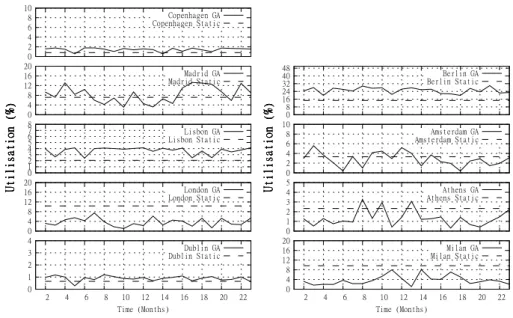
In Figure 8(b) we break this renewable energy usage down across individual data-centres. As expected, the change in renewable energy used varies from data-centre to data-centre, depending on its renewable ratio. Many data centres (e.g. Lisbon, Copenhagen, Berlin) increase their renewable usage while others (e.g. London, Milan, Athens) perform worse, using more fossil-fuel based energy. Increases in renewable energy are a result of more favourable conditions (i.e. higher renewable ratios) in that country and vice versa. We can see a strong correlation here with the utilisation as indicated in Figure 11, as data centres that increase utilisation also increase renewable energy utilisation, while those with lower utilisation decrease renewable usage. Correlation can also be seen with
0 2000 4000 6000 8000 10000 12000 14000 16000 18000 5 10 15 20 Re newa ble Ener gy ( MWh ) Time (months)
GA Total Renewable Energy Static Total Renewable Energy
(a) 0 100 200 300 400 500 2 4 6 8 10 12 14 16 18 20 22 Time (Months) Renewable Energy (MWh ) Dublin GA Dublin Static 0 200 400 600 800 1000 Renewable Energy (MWh ) London GA London Static 0 500 1000 1500 2000 2500 3000 Renewable Energy (MWh ) Lisbon GA Lisbon Static 0 1000 2000 3000 4000 5000 Renewable Energy (MWh
) Madrid StaticMadrid GA
0 500 1000 1500 2000 2 4 6 8 10 12 14 16 18 20 22 Time (Months) Renewable Energy (MWh ) Milan GA Milan Static 0 100 200 300 400 500 Renewable Energy (MWh ) Athens GA Athens Static 0 150 300 450 600 750 Renewable Energy (MWh ) Amsterdam GA Amsterdam Static 0 2000 4000 6000 8000 10000 12000 Renewable Energy (MWh
) Berlin StaticBerlin GA
0 500 1000 1500 2000 Renewable Energy (MWh ) Copenhagen GA Copenhagen Static (b)
6e+007 6.5e+007 7e+007 1 2 3 4 5 6 7 8 9 10 11 12 13 14 15 16 17 18 19 20 21 22 23 CO 2 (K g) Time (Months) GA CO2 Static CO2
Figure 9 CO2 Emissions
the renewable ratios in Figure 6(b), as those with higher renewable ratios gain renewable energy and vice versa.
In Figure 9 we present an indicative graph of potential CO2emissions based on
the quantity of renewable and fossil based fuels used by each simulation. According to the UK Department of Environment, Food and Rural Affairs (DEFRA) the average volume of CO2 produced by consuming a KWh of electricity (produced
using fossil fuels) in the UK is 0.54160KG. Using this figure as a guideline we can directly translate our usage of fossil-based energy to CO2 emissions. Given the
stated figure of 1566MWh per month (average) this would equate to a monthly average of 848545KG (or 848 metric tonnes) of CO2.
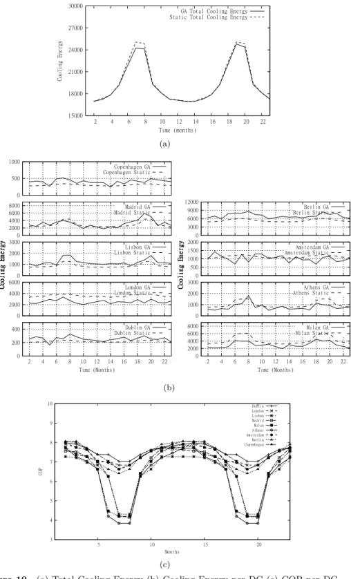
In Figure 10(a) we present the total cooling energy used by both the genetic algorithm and static simulations. In the fitness function we aim to minimize the cooling energy expended, where cooling energy is directly proportionate to the COP of the data centre and the load exerted on the data centre. Savings are made by moving load to countries with lower temperatures and hence better COP values. If there is no significant variance in the temperatures of the countries then there is little opportunity to make significant savings. In Figure 10(c) we can see that, during the winter periods the COP values for each data centre are very close and so the savings observed are very small. During the summer periods the COP values diverge and so the GA finds service placements that provide energy savings. In general however the savings observed for cooling energy are small (at best 3% for months 6-8), and this is due to the geographic proximity of the data-centres.
In Figure 10(b) cooling energy values for each individual data centre are shown. Again there is a strong correlation here with the utilisation values in Figure 11, where DCs with higher utilisation will see higher cooling energy. The cooling energy values may appear somewhat counter-intuitive at first, given that the data-centres with the best COPs generally show increased cooling energy values for the GA (e.g. Dublin, Copenhagen, Berlin). However, given that the data centres with the best COP values are targeted for service placement, this will lead to increased utilisation and hence increased cooling energy usage. Since these have the most efficient cooling conditions, the cooling cost is lower than on those data
15000 18000 21000 24000 27000 30000 2 4 6 8 10 12 14 16 18 20 22 Co olin g En ergy Time (months)
GA Total Cooling Energy Static Total Cooling Energy
(a) 0 200 400 2 4 6 8 10 12 14 16 18 20 22 Time (Months) Co oli ng En erg y Dublin GA Dublin Static 0 2000 4000 6000 Co oli ng En erg y London GA London Static 0 1000 2000 3000 Co oli ng En erg y Lisbon GA Lisbon Static 0 2000 4000 6000 8000 Co oli ng En erg y Madrid GA Madrid Static 0 2000 4000 6000 8000 2 4 6 8 10 12 14 16 18 20 22 Time (Months) Co oli ng En erg y Milan GA Milan Static 0 1000 2000 3000 Co oli ng En erg y Athens GA Athens Static 0 500 1000 1500 2000 Co oli ng En erg y Amsterdam GA Amsterdam Static 0 3000 6000 9000 12000 Co oli ng En erg y Berlin GA Berlin Static 0 500 1000 Co oli ng En erg y Copenhagen GA Copenhagen Static (b) 3 4 5 6 7 8 9 10 5 10 15 20 COP Months Dublin London Lisbon Madrid Milan Athens Amsterdam Berlin Copenhagen (c)
0 1 2 3 4 2 4 6 8 10 12 14 16 18 20 22 Time (Months) Utilisation (%) Dublin GA Dublin Static 0 4 8 12 16 20 Utilisation (%) London GA London Static 0 1 2 3 4 5 6 7 8 Utilisation (%) Lisbon GA Lisbon Static 0 4 8 12 16 20 Utilisation (%) Madrid GA Madrid Static 0 4 8 12 16 20 2 4 6 8 10 12 14 16 18 20 22 Time (Months) Utilisation (%) Milan GA Milan Static 0 1 2 3 4 5 Utilisation (%) Athens GA Athens Static 0 2 4 6 8 10 Utilisation (%) Amsterdam GA Amsterdam Static 0 8 16 24 32 40 48 Utilisation (%) Berlin GA Berlin Static 0 2 4 6 8 10 Utilisation (%) Copenhagen GA Copenhagen Static
Figure 11 Utilisation per DC
centres with higher COPs for the same load. In other words, by removing load from lower-efficiency data centres and placing it on more efficient data centres we reduce the cooling energy consumed. There are some exceptions though, such as London and Amsterdam, who generally have good COP values but their cooling values do not necessarily reflect this. However we must consider the effects of the renewable aspect of the fitness function. Dublin, Copenhagen and Berlin also have good or very good renewable energy ratios, which make them more attractive for placement (i.e. higher fitness) while London and Amsterdam have poor or very poor renewable values. This offsets the effect of a positive COP value.
Figure 11 presents the utilisation experienced by each data centre over the course of the simulation. The utilisation values presented here are relative to the overall capacity of the entire data-centre group (i.e. all 9 data centres). As expected we can see that many of the data centres in the GA approach decrease capacity compared to the static while others increase. The data centres that consistently increase (Copenhagen, Lisbon, Dublin, Berlin) can be seen to correspond to those data centres that perform well in terms of renewable energy and also cooling energy. It must be noted that utilisation is also influenced by the capacity of the data centres. For instance Copenhagen is generally the best performer in terms of renewable energy and one of the top performers for cooling, yet Berlins utilisation increase is significantly larger. This is simply because Berlin is a considerably larger data centre and can handle a much larger utilisation increase. In terms of reduced utilisation, we can see that London and Milan show significant reductions with Athens, Amsterdam and Madrid show varying levels of reduction. For London and Milan, both have very poor renewable energy ratios (specifically London).
Finally in Figure 12 we show the cost values incurred in both simulations. Since cost is not part of the fitness function this is presented only to evaluate the
13000 14000 15000 1 2 3 4 5 6 7 8 9 10 11 12 13 14 15 16 17 18 19 20 21 22 23 Co st ( Euro ) Time (Months) Totol Cost GA Totol Cost Static
Figure 12 Total Cost
cost impact of our solution. Here it can be seen that the cost of our solution is lower than the cost of the static approach. However the cost decrease is very small (approx. 2.5% average), but the aim here is not to considerably reduce the cost, merely to ensure that our proposed approach does not come at a financial burden to the data centre operator. This is important in promoting the proposed solution to data centres operators, as increased costs will negatively impact the renewable energy benefits of the system.
4.3 Simulation Set B
In our second set of simulations we adapt a fluctuating traffic profile to evaluate the ability of the GA to react dynamically to changes in its dependant parameters (e.g. service request levels or weather patterns). In order to model the service request profile of a realistic data-centre operator we adopt the basic traffic profile from the Akamai data centres discussed in (Qureshi and Weber, 2009). We extrapolated the weekly traffic view over the course of 12 months. To model the potential dynamicity of service requests we added a number of randomly distributed surges and falls in the request rate to represent changes in service usage (Figure 13). The average request rate is two million requests per day.
In Figure 14(a) we present the levels of renewable energy consumed by both the GA-based service migration approach and the case where services do not migrate (static). As described earlier, the aim here is to maximize the amount of renewable energy consumed by moving load to countries with higher levels of renewable energy production, while also considering the cooling energy depending on the weather of that country. Also, for the GA-based approach we present two variations in terms of the GA triggering, including a dynamically triggered and a fixed bi-weekly execution. We choose a bi-weekly schedule to compare against as we felt that this was the highest frequency schedule reasonable (i.e. weekly would have been too frequent).
Firstly we can see that both simulations using the genetic algorithm considerably improved the quantity of renewable energy consumed. On average there is a 15.2% renewable energy difference between the optimized and non-optimized configurations, accounting for 1440MWh of energy per month. These values are largely in line with those described in Set A using a flat traffic profile.
0 100000 200000 300000 400000 500000 600000 50 100 150 200 250 300 350 Service Requests Time (Days) Dublin London Lisbon Madris Milan Athens Amsterdam Berlin Copenhagen
Figure 13 Service Request Rates
In terms of the GA execution schedule, our aim is to evaluate whether intelligently triggering the GA can lead to comparable or even improved performance over a fixed execution schedule, while at the same time running the GA less frequently. In essence, every GA execution leads to a re-configuration of the service data-centre placement. This re-configuration does not come without a cost. The services have to be physically moved to their new location, consuming bandwidth, as well as the management overheads in relocating services. Finally then, service requests and traffic must be forwarded from/to the originating data centre to the new service location. It is clear then that minimizing number of reconfigurations is desirable.
The gains that we attempt to make here are achieved not by HOW the GA runs but rather WHEN the GA runs. After a GA execution, the service configuration is optimal for that specific time period. However, as time progresses the request rate and energy values may change somewhat rendering the service configuration no longer optimal. If this variation is small then there would be little opportunity for gainful reconfigurations. By attempting to run the GA only when significant changes have occurred it should be possible to perform as well as a fixed, regularly executing GA. Indeed we can see that, in general, the dynamically triggered GA performs slightly better than the fixed execution. When both GAs run at the same time (GA execution is indicated with a point) they have largely comparable energy values (e.g. time 11). However, when the dynamic GA runs at a time period where the bi-weekly GA does not it typically improves the renewable energy values (e.g. times 32, 60, 116). In total the improvements gained by the dynamic GA are very small (approx. <1%, or 668MWh over the duration of the simulation). However the dynamic GA executed only 15 times, as compared to the bi-weekly executions 26 times. In terms of the performance of the triggering algorithm, we can see that, for instance, the GA execution on days 95 and 230 are clearly as a result of the large request spikes in Berlin at the same times (Figure 13). In Figure 14(b) we examine the renewable energy consumed in each data-centre using both the dynamic and the bi-monthly GA. As we would expect, following on from Figure 14(a), the dynamic and bi-weekly levels for each data-centre are relatively close.
200 250 300 350 400 450 500 20 40 60 80 100 120 140 160 180 200 220 240 260 280 300 320 340 360 Renewable Energy (MWh ) Time (Days) Dots represent GA Execution
Dynamic GA Dynamic Execution Bi-Monthly GA Bi-Monthly Execution Static Services (a) 0 10 20 30 40 50 30 60 90 120 150 180 210 240 270 300 330 360 Time (Days) Re new ab le Ene rgy Re new ab le Ene rgy Dublin GA Dublin Bi-Monthly 0 10 20 30 40 50 Re new ab le Ene rgy Re new ab le Ene rgy London GA London Bi-Monthly 0 20 40 60 80 100 Re new ab le Ene rgy Re new ab le Ene rgy Lisbon GA Lisbon Bi-Monthly 0 50 100 150 200 Re new ab le Ene rgy Re new ab le Ene rgy Madrid GA Madrid Bi-Monthly 0 20 40 60 80 100 30 60 90 120 150 180 210 240 270 300 330 360 Time (Months) Re new ab le Ene rgy Re new ab le Ene rgy Milan GA Milan Bi-Monthly 0 5 10 15 20 25 30 Re new ab le Ene rgy Re new ab le Ene rgy Athens GA Athens Bi-Monthly 0 20 40 60 80 100 Re new ab le Ene rgy Re new ab le Ene rgy Amsterdam GA Amsterdam Bi-Monthly 0 100 200 300 400 Re new ab le Ene rgy Re new ab le Ene rgy Berlin GA Berlin Bi-Monthly 0 10 20 30 40 50 Re new ab le Ene rgy Re new ab le Ene rgy Copenhagen GA Copenhagen Bi-Monthly (b)
Figure 14 (a) Static Renewable Energy v Dynamic and Biweekly (b) Renewable
600 700 800 900 1000 1100 50 100 150 200 250 300 350 Co olin g En ergy MWh Time (Days) GA Static (a) 0 10 20 30 40 50 30 60 90 120 150 180 210 240 270 300 330 360 Time (Days) Cooling Energy Dublin GA Dublin Static 0 100 200 300 400
Cooling Energy London GA London Static 0 20 40 60 80 100 Cooling Energy Lisbon GA Lisbon Static 0 100 200 300 400 Cooling Energy Madrid GA Madrid Static 0 100 200 300 400 30 60 90 120 150 180 210 240 270 300 330 360 Time (Days) Cooling Energy Milan GA Milan Static 0 20 40 60 80 100
Cooling Energy Athens GA Athens Static 0 20 40 60 80 100 Cooling Energy Amsterdam GA Amsterdam Static 0 100 200 300 400 500 Cooling Energy Berlin GA Berlin Static 0 10 20 30 40 50 Cooling Energy Copenhagen GA Copenhagen Static (b)
2.25e+006 2.4e+006 2.55e+006 21 42 63 84 105 126 147 168 189 210 231 252 273 294 315 336 357 CO 2 (K g) Time (Days) GA CO2 Static CO2
Figure 16 CO2 Emissions
In Figure 16, (like Figure 9 before), we convert the gains made in renewable energy to the equivalent CO2 emissions. Using the same guideline value (.54160kg/KWh), we see that the dynamic GA reduces the volume of CO2
emissions over the static (note we did note show bi-weekly as the emissions values are very close). The average reduction amounts to 25943kg of CO2 per day across
all data-centres. As would be expected the rates follow the variation in the service request rate, given that this drives the energy usage within the data-centre.
We now present the cooling energy values for the both the GA and static simulations in Figure 15(a) and 15(b). As we discussed for Set A, gains in cooling energy are difficult to achieve for the data-centres used in this case-study, as the temperature profiles are simply too similar for the majority of the year to achieve any real saving. We can see again that we only make gains in the summer when temperature profiles are higher and diverge somewhat. In Figure 15(b) we show the cooling energy required for each data-centre. As we can see, there is once again a strong correlation with utilisation values for each data-centre and also with the cooling energy observed in simulation set one. Data-centres with more efficient cooling (i.e. higher COP values - see Figure 10(c)), increase in cooling energy as they are targeted for service placement. However the cooling energy expended at these data-centres is smaller than would be expended in less efficient data-centres, for an equivalent service load.
In Figure 17 we show the utilization values for each data-centre. The behaviour overall, as would be expected, replicates the behaviour of set A, with Berlin, Lisbon and Copenhagen all increasing in utilisation, while London and Milan show significantly large reductions. The reasons for this are the same as discussed in Section 4.2. Even though the traffic patterns might be different, the countries that perform well in terms of renewable energy and cooling efficiency remain the same. We can see that the peaks/troughs effect utilisation in the static plots, however in the GA plots this is more difficult as increased requests at one data-centre may effect the services in another, since requests are forwarded to the new location of the service.
Finally, in Figure 18, we show the cost associated with the dynamic, bi-weekly and static simulations. Like the cost from Set A, both GA-based simulations
0 1 2 3 30 60 90 120 150 180 210 240 270 300 330 360 Time (Days) Utilisation (%) Dublin GA Dublin Static 0 5 10 15 20 25 Utilisation (%) London GA London Static 0 2 4 6 8 10 Utilisation (%) Lisbon GA Lisbon Static 0 5 10 15 20 25 Utilisation (%) Madrid GA Madrid Static 0 5 10 15 20 25 Time (Days) Utilisation (%) Milan GA Milan Static 0 1 2 3 4 5 Utilisation (%) Athens GA Athens Static 0 2 4 6 8 10 Utilisation (%) Amsterdam GA Amsterdam Static 0 10 20 30 40 50 Utilisation (%) Berlin GA Berlin Static 0 1 2 3 4 5 Utilisation (%) Copenhagen GA Copenhagen Static
Figure 17 Utilisation per DC
(dynamic and bi-weekly) cost slightly less than the static. The bi-weekly and dynamic GAs have effectively the same average cost overall, with dynamic being slightly cheaper than bi-weekly (by 0.4%). This correlates to the renewable energy values also in that the dynamic was less than 1% better that bi-weekly.
5 Discussion and Future Work
Here we will briefly discuss some issues that we feel warrant highlighting. Firstly, we abstract the energy grid of each country to be a ’black box’, where we assume each energy source is fed into the grid and its source becomes indiscernible. In other words, the energy produced from renewable sources is not partitioned or reserved for specific usage, but is available in the grid for common usage in direct proportion to the rate at which it was produced. Another issue that we discuss here is the additional energy and latency costs that may be incurred by moving quantities of services between data centres. Moving services could cause higher loads on networking equipment along the migration path, hence increasing their energy consumption. Also, moving services further from the source of requests could potentially increase delays times and hence reduce end user Quality of Experience (QoE). In future work we plan to expand our simulations to evaluate these effects on the underlying network infrastructure. However, we feel that these effects could be limited by placing a distance limit on migrating services or indeed integrating a distance metric directly into the fitness function itself. In this way we could ensure that we always attempt to minimise the effects of migration on energy and QoS.
400 450 500 550 600 50 100 150 200 250 300 350 Co st ( Euro ) Time (Months)
Total Cost Dynamic GA Total Cost BiWeek GA Total Cost Static
Figure 18 Total Cost
6 Conclusion
Due to the increasing popularity of the Internet, the communication systems of the future are predicted to consume large quantities of energy. In particular, the data centres that house various types of Internet services are poised to be the most significant consumer of energy. While improving energy efficiency is one objective of modern society, another key objective is to move towards green, renewable energy sources to reduce our carbon footprint. In this paper we have proposed a green data centre solution that uses a GA-based service placement approach based on targeting countries with the highest production of renewable energy and the best conditions for cooling. To validate our proposed solution, we carried out some demonstrative simulations by gathering data regarding the renewable energy production and temperature profiles of each country, and implementing a genetic algorithm that aims to maximise the quantity of renewable energy consumed and minimise cooling energy expended. From our simulations we have demonstrated that by employing this technique it is feasible to make significant improvements in the proportion of renewable energy utilised in data centre operation, hence reducing the quantity of fossil fuels burned and ultimately carbon emissions. We also demonstrated that cooling energy can be reduced in circumstances where there is significant variance in the countrys temperature profiles. At the same time, we showed that this improved renewable energy utilisation did not come at an increased monetary cost for the operator.
Acknowledgements
The authors wish to acknowledge the following funding support: Science Foundation Ireland under Grant Number 08/SRC/I1403 (Federated, Autonomic Management of End-to-End Communications Services), and Science Foundation Ireland under Grant Number 09/SIRG/I1643 (A Biologically inspired framework supporting network management for the Future Internet).
References
Balasubramaniam, S., Botvich, D., Carroll, R., Mineraud, J., Nakano, T., Suda, T., Donnelly, W. (2009), ’Adaptive Dynamic Routing Supporting Service Management for Future Internet’, In proceedings of the Global Communication Conference (Globecom) 2009, Hawaii.
Energy Star (2007). ’Report to Congress on Server and Data Center Energy Efficiency Public Law 109-431’. Washington, D.C.: U.S. Environmental Protection Agency, available at http://www.energystar.gov/ia/partners/prod development/downloads/EPA
Datacenter Report Congress Final1.pdf.
Bradley, D. J., Harper, R. E. and Hunter, S. W (2003) ’Workload-based Power Management for Parallel Computer Systems’. IBM Journal of Research and Development, Vol. 47, pp.703-718.
Das, R., Kephart, J. O., Lefurgy, C., Tesauro, G., Levine, D. W., and Chan, H. (2008) Autonomic multi-agent management of power and performance in data centers. In The Seventh International Conference of Autonomic Agents and Multiagent Systems
Meisner, D., Gold, B. T., and Wenisch, T. F.,(2009) ’PowerNap: Eliminating Server Idle power’, in ACM SPLOS
Rusu, C. et al (2006) Energy-Effcient Real-Time Heterogeneous Server Clusters. In Proceedings of RTAS, April 2006.
Barbagallo, D., Nitto, E. Di, Dubois, D. J. , Mirandola, R. (2010), ’A Bio-Inspired Algorithm for Energy Optimization in a organizing Data Center’. Self-Organizing Architectures, Springer.
Moore, J., Chase, J., Ranganathan, P., Sharma, R. (2005) ’Making scheduling ”cool”: temperature-aware workload placement in data centers’, Proceedings of the USENIX Annual Technical Conference 2005 on USENIX Annual Technical Conference, p.5-5, April 10-15, Anaheim, CA
Patel, C.D., Sharma, R.K, Bash, C.E. and Graupner, S., (2003) ’Energy Aware Grid: Global Workload Placement based on Energy Efficiency’, IMECE 2003-41443, 2003 International Mechanical Engineering Congress and Exposition, Washington, DC.
Bash, C., and Forman, G., (2007). ’Cool job allocation: Measuring the power savings of placing jobs at cooling-efficient locations in the data center’. In Proceedings of the USENIX Annual Technical Conference, pp. 363368.
Wang, L. et al.(2009), ’Towards Thermal Aware Workload Scheduling in a Data Center’. In Proceedings of the 10th International Symposium on Pervasive Systems, Algorithms and Networks (IS-PAN2009), Kao-Hsiung, Taiwan, 14-16 December.
Sharma, R. et al (2005), ’Balance of Power: Dynamic Thermal Management for Internet Data Centers’. IEEE Internet Computing, 9(1):42-49, January.
Tang, Q., Gupta, S.K.S., Varsamopoulos, G. (2008), ’Energy-Efficient Thermal-Aware Task Scheduling for Homogeneous High-Performance Computing Data Centers: A Cyber-Physical Approach’ IEEE Transactions on Parallel and Distributed Systems, VOL. 19, NO. 11, November 2008
Garg, S. K., Yeo, C. S., Anandasivam, A. and Buyya, R. (2010) ’Environment-conscious scheduling of HPC applications on distributed cloud-oriented data centers’, Journal of Parallel and Distributed Computing.
Qureshi, A., Weber, R et al. ’Cutting the Electric Bill for Internet-Scale Systems’, SIGCOMM09, August 1721, 2009, Barcelona, Spain.
Moran, M. J. and Shapiro, H. N. (1995), ’Fundamentals of Engineering Thermodynamics’, Wiley, New York
Oakridge National Laboratory (ORNL) Heat Pump Model, availabel at http://www.ornl.gov/ wlj/hpdm/MarkVII.shtml
International Energy Agency,http://www.iea.org
European Climate Assessment & Dataset (ECA&D),http://eca.knmi.nl/ European Commission: Eurostat,http://epp.eurostat.ec.europa.eu/