Increasing rendering performance of graphics hardware

(1)

INCREASING RENDERING PERFORMANCE OF GRAPHICS HARDWARE

Justin Hensley

A dissertation submitted to the faculty of the University of North Carolina at Chapel Hill in partial fulfillment of the requirements for the degree of Doctor of Philosophy in the Department of Computer Science.

Chapel Hill 2007

Approved by:

Anselmo Lastra

Montek Singh

Mary Whitton

Leonard McMillan

(2)

c

2007

(3)

ABSTRACT

JUSTIN HENSLEY: Increasing Rendering Performance of Graphics Hardware (Under the direction of Anselmo Lastra and Montek Singh)

Graphics Processing Unit (GPU) performance is increasing faster than central processing unit (CPU) performance. This growth is driven by performance improvements that can be divided into the following three categories: algorithmic improvements, architectural improve-ments, and circuit-level improvements. In this dissertation I present techniques that improve the rendering performance of graphics hardware measured in speed, power consumption or image quality in each of these three areas.

At the algorithmic level, I introduce a method for using graphics hardware to rapidly and efficiently generate summed-area tables, which are data structures that hold pre-computed two-dimensional integrals of subsets of a given image, and present several novel rendering techniques that take advantage of summed-area tables to produce dynamic, high-quality im-ages at interactive frame rates. These techniques improve the visual quality of imim-ages rendered on current commodity GPUs without requiring modifications to the underlying hardware or architecture.

At the architectural level, I propose modifications to the architecture of current GPUs that add conditional streaming capabilities. I describe a novel GPU-based ray-tracing algo-rithm that takes advantage of conditional output streams to reduce the memory bandwidth requirements by over an order of magnitude times when compared to previous techniques.

At the circuit level, I propose acompute-on-demand paradigm for the design of high-speed and energy-efficient graphics components. The goal of the compute-on-demand paradigm is to only perform computation at the bit-level when needed. The compute-on-demand paradigm exploits the data-dependent nature of computation, and thereby obtains speed and energy im-provements by optimizing designs for the common case. This approach is illustrated with the

(4)

design of a high-speed Z-comparator that is implemented using asynchronous logic. Asyn-chronous or “clockless” circuits were chosen for my implementations since they allow for data-dependent completion times and reduced power consumption by disabling inactive com-ponents. The resulting circuit-level implementation runs over 1.5 times faster while on dissi-pating 25% the energy of a comparable synchronous comparator for the average case.

(5)

In memory of my brother, Jeff Hensley. As children we didn’t always get along, and I regret not being able to tell you how much you meant to me. I love you and I miss you.

(6)

ACKNOWLEDGMENTS

Ever since I can remember, I have always wanted to get my Ph.D. As a young child, I would often inform people that I was going to get my doctorate in aeronautical engineering. Since you are currently reading this dissertation, it should be fairly clear to you that I did not in fact get my Ph.D. in aeronautical engineering. If you are expecting a treatise on airplane design, you are gravely mistaken. Despite this minor change in plans, I have always known that I would be going to college, even from an early age. I believe that I have my parents to thank for this. There was never a question about whether I would go to college. My parents always supported me, and always wanted me to do my best, whatever it was that I chose to do. For their unwavering support, I would like to thank my parents.

My journey through college has been filled with some of the happiest times of my life, and some of the saddest times of my life. As an undergraduate, I was fortunate enough to live in a small dorm at the University of California at Davis. It is there that I met Ami, the love of my life, an amazing woman, who, when I asked her to marry me, said yes. She was willing to transfer universities in the middle of her veterinary medical program so that we could be together after the we got married. I know that it was difficult for Ami to leave her friends at Purdue to attend North Carolina State University, and for her sacrifice I am eternally grateful, since I know that I would not have been able to finish this dissertation without her support. For being there when it mattered most for me, thank you Ami. 1

As an undergraduate, I originally started out in the biosystems engineering program at UC Davis. It did not take long, one quarter in fact, for me to decide that biosystem engineering was not for me. Suffice to say, the course that led to my decision involved learning about mass producing bean sprouts, and I have always known that I didnot want to work in agriculture. Sorry dad. After filling out the requisite forms, I was soon majoring in computer science and

1

(7)

electrical engineering. When I got my first introduction to computer graphics, I was well on my way to becoming a computer architect, but after taking ”Introduction to Computer Graphics” with Professor Ken Joy, I knew that I wanted to work with computer graphics. I would like to thank Professor Joy for introducing me to the field of computer graphics, and for his encouragement to attend UNC for my doctorate degree.

At UNC, I initially joined the “Office of the Future” research group, and began working on what was eventually named PixelFlex. As a member of OOTF I was advised by Herman Towles and Henry Fuchs. I am grateful for the guidance they gave me during my first two years at UNC, but as fate would have it one tragic day I received a phone call that my brother had died. In a single moment, my life had changed forever. While I know it is trite to say that, there are no other ways I can describe how I felt on that day and how I still feel.

My co-advisors Montek Singh and Anselmo Lastra have been invaluable to me. All of the research I have done since leaving the PixelFlex project has been under their supervision. For the past four years, the endpoint of my research has not always been sight; Anselmo and Montek have been there to help me through the rough patches. For their support and guidance, I would like to thank my co-advisors.

To the rest of my committee, Leonard, Mary, and Steve: I would like to thank you for your advice and guidance. To my friends at UNC, thank you for the support and friendship you have given me. Finally, I would also like to thank the many foosball players in the department who helped me keep my sanity.

(8)

LIST OF TABLES

2.1 Shortest time to generate summed-area tables of different sizes . . . 28 2.2 Time to generate summed-area tables using different number of samples per pass 28

3.1 Comparison of our technique with the results presented by Foley and Sugerman 56 3.2 Scatter performance using GL POINTS with a vertex shader on an ATI X1900XT 59

4.1 24-bit Comparator results . . . 80

(14)

LIST OF FIGURES

1.1 Sampling from summed-area tables . . . 4

1.2 Glossy environmental reflections using summed-area tables . . . 5

1.3 Conditional operations with streaming architectures . . . 7

1.4 Synchronous and asynchronous system block diagrams . . . 10

1.5 Distribution of z-comparison compute chain length . . . 11

2.1 Planar reflection mapping . . . 16

2.2 Dual-paraboloid maps . . . 18

2.3 Image-based lighting . . . 20

2.4 The recursive doubling algorithm in 1D . . . 24

2.5 Effects of precision loss with summed-area tables . . . 30

2.6 Summed-area table reconstruction error . . . 32

2.7 Comparison of images filtered using repeated offset summed-area tables . . . 33

2.8 An object rendered with glossy reflections by filtering a dynamic environment map with a spatially varying kernel size . . . 35

2.9 An object textured using four samples from a pair of summed-area tables . . 36

2.10 A set of four box filters stacked to approximate a Phong BRDF . . . 37

2.11 An image illustrating the use of a summed-area table to render glossy planar reflections . . . 38

2.12 Simulated depth-of-field effect using summed-area tables . . . 40

2.13 Example of translucency using a summed-area table . . . 41

2.14 Approximate image-based lighting computed from two sets of summed area tables . . . 43

2.15 Approximating a diffuse BRDF using summed area tables . . . 44

3.1 Ray traced second generation rays using conditional output streams . . . 47

3.2 Conditional operations with streaming architectures . . . 50

(15)

3.4 Additional hardware needed to implement conditional streams in graphics

hardware . . . 52

3.5 Processing time per pass for kd-tree node traversal GLSL shader . . . 57

3.6 Effective processing time per ray for traversal shader . . . 58

4.1 Synchronous and asynchronous systems (figure adapted from (Singh, 2001)). 61 4.2 Examples of handshake schemes . . . 63

4.3 A bundled data function block . . . 64

4.4 A dual-rail data encoding scheme . . . 65

4.5 A dual-rail AND gate in dynamic logic . . . 67

4.6 A dynamic logic gate (figure adapted from (Singh, 2001)). . . 68

4.7 Block diagram of a PS0pipeline . . . 69

4.8 The high-capacity (HC) pipeline style . . . 71

4.9 A frame from Unreal Tournament 2004 . . . 76

4.10 A novel “compute-on-demand” comparator . . . 79

4.11 Distribution of z-comparison compute chain length for the frame shown in Figure 4.9 . . . 81

4.12 The counterflow Booth multiplier . . . 85

4.13 The merged arithmetic/shift unit . . . 88

4.14 Pipeline Handshake Controller . . . 90

4.15 Booth Controller . . . 94

4.16 Booth commands . . . 94

4.17 The variable-precision Booth multiplier architecture . . . 96

4.18 Pipeline Handshake Controller . . . 98

(16)

LIST OF ABBREVIATIONS

2D Two-Dimensional 3D Three-Dimensional CPU Central Processing Unit

DRAM Dynamic Random Access Memory GPU Graphics Processing Unit

HC High-Capacity

(17)

CHAPTER 1

Introduction

Graphics Processing Unit (Graphics Processing Unit (GPU)) performance is increasing faster than Central Processing Unit (Central Processing Unit (CPU)) performance, and is reported by some to be growing at a “Super-Moore’s Law” rate (Govindaraju et al., 2006). This growth is driven by performance improvements that can be divided into the following three categories.

• Algorithmic: Algorithmic improvements are often initially implemented at the appli-cation level, using the current capabilities of current hardware. The relatively recent introduction of programmable pipelines to commodity GPUs enables a wide variety of algorithms to be implemented without architectural changes.

• Architectural: There are situations where a new algorithm lends itself to an efficient, direct implementation in hardware that would require only minimal changes to the GPUs architecture. For example, various environment mapping techniques initially required the application developer to handle texture coordinate generation, whereas modern GPUs are able to automatically transform normal and reflection directions into texture coordinates.

(18)

• Circuit: At the circuit level, it is possible to make dramatic changes to the underly-ing circuitry without modifyunderly-ing the GPU’s architecture or the application programmer interface. Some of the possible benefits of circuit-level modifications include faster com-putation, lower energy-consumption, or improved yields when fabricating integrated circuits. For example, some modern hardware has moved from using standard-cell im-plementations to custom ASICs without requiring changes to the overall architecture. Also, over the lifetime of a specific architecture, multiple different fabrication processes might be used — e.g. a device might initially be implemented in a 90 nm process, but later be fabricated in a 65 nm process as the architecture and fabrication processes become more mature.

Performance improvements can be measured in several ways. In this work I use metrics related to the visual image quality, speed of computation, and energy-efficiency. The following sections give more detail about the contributions made in these three areas.

1.1 The Algorithmic Axis: Improving Rendering Quality with

GPU-Based Summed-Area Tables and Extensions

At the algorithmic level, I will discuss several novel techniques that are capable of improving the visual quality of images rendered on current commodity GPUs without requiring modi-fications to the underlying hardware or architecture. In particular, I will describe a method for using graphics hardware to rapidly and efficiently generatesummed-area tables, which are data structures that hold pre-computed integrals of a given image. Additionally, I will de-scribe extensions to summed area tables that reduce their precision requirements and present multiple rendering techniques that take advantage of summed-area tables to produce high-quality images in real-time. My algorithm is able to compute a 256x256 summed-area table in less than 2ms, and render complex scenes, such as the one shown in Figure 1.2(a), with interactive glossy reflections at over 60 frames per second on relatively old hardware such as a Radeon X800XT PE.

(19)

summed-area tables. Readers familiar with the topics can skip to Section 1.1.2.

1.1.1 Background

Texture mapping, a technique that is ubiquitous in computer graphics, is a process that enables simple rendered surfaces to appear to have complex surface properties. In its simplest form, texture mapping can be thought of as an image being used as a decal on the surface of an object. Introduced by Catmull (Catmull, 1974), texture mapping is a process whereby positions in three-space are mapped to an n-dimensional, parametric space, which allows for easy sampling of data stored in n-dimensional arrays such as images (2D) and volumetric data (3D).

As with any sampling technique, it is often necessary to filter or interpolate the data sam-pled from a texture map to attain visually pleasing images. In practice, it is cost-prohibitive to directly interpolate the texture map with anything more complex than linear interpolation. Mipmaps (Williams, 1983) address this issue by pre-computing multiple images, which are scaled-down versions of the original input image, and then performing trilinear interpolation between two levels of the mipmap.

First introduced by Crow (Crow, 1984), summed-area tables enable more general tex-ture filtering than is possible with the commonly-used mipmapping technique. In particular, summed-area tables are able to more accurately reflect the data actually inside a box filter kernel at a specific location, whereas a nearby samples from a mipmap are limited to the average of a fixed set a pixels. When using a mipmap to perform more generalized filtering, this becomes apparent as visual defects in the filtered image. Although introduced at roughly the same time as mipmaps, summed-area tables have a more stringent precision requirement than an equivalently sized mipmap. Partly due to this limitation of summed-area tables, mipmapping became a more attractive technique to implement in early GPUs, and summed-area tables fell out of favor in real-time rendering. But, summed-summed-area tables remained a useful technique in offline rendering applications such as the renders used in the film industry. The relatively recent availability of floating-point capable datapaths, and the associated increase in the available computational precision on commodity GPUs has facilitated a resurrection in

(20)

X

_L

X

_R

Y

_T

Y

_B

Figure 1.1: (after [Crow84]) An entry in the summed-area table holds the sum of the values from the lower left corner of the image to the current location. To compute the sum of the dark rectangular region, evaluateT[XR, YT]−T[XR, YB]−T[XL, YT] +T[XL, YB] where T is

the value of the entry at (x, y).

the use of summed-area tables in real-time graphics, despite their high precision requirements. For an image, a summed-area table is a two-dimensional array where each entry in the array stores the discrete integral for each rectangular sub-image of the input image. Summed-area tables enable at a fixed computational cost the rapid calculation of the sum of the pixel values in an arbitrarily sized, axis-aligned rectangle. Figure 1.1 illustrates how a summed-area table is used to compute the sum of the values of pixels spanning a rectangular region. To find the integral of the values in the dark rectangle, we begin with the pre-computed integral from (0,0) to (xR, yT). We subtract the integrals of the rectangles (0, 0) to (xR, yB) and (0,

0) to (xL, yT). The integral of the hatched box is then added to compensate for having been

subtracted twice. Finally, the average value of a group of pixels can be calculated by dividing the sum by the area.

(21)

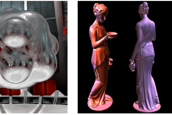
(a) Glossy environmental reflections (b) Approximate HDR image-based lighting Figure 1.2: Image (a) shows an object rendered in real-time with an environment map fil-tered by a spatially varying filter. Image (b) shows A real-time rendering of a statue of Hebe, the Greek goddess of youth. All lighting calculations are only performed by sampling summed-area tables computed from the Grace Cathedral lightprobe (lightprobe courtesy of Paul Debevec). The left image of Hebe shows an approximation to the Phong BRDF, and the right image shows an approximation to a diffuse BRDF.

handle complex filter functions by taking advantage of the properties of convolution. These extensions will be described in more detail in Chapter 2.

1.1.2 Contributions

In this dissertation I present a method to rapidly generate summed-area tables that is efficient enough to allow multiple summed-area tables to be generated every frame while maintain-ing interactive frame rates. I extend the traditional summed-area table algorithm to reduce their precision requirements, which enables summed-area tables to easily be used on graphics hardware with relatively limited-precision, or alternatively, larger summed-area tables to be generated with visual artifacts being introduced. I demonstrate the applicability of spatially varying filters for real-time, interactive computer graphics through several different applica-tions. Some example applications are the interactive rendering of dynamic glossy reflections

(22)

(Hensley et al., 2005), and dynamic image-based lighting (Hensley et al., 2006). Figure 1.2(a) shows an image captured from a real-time application that is rendering an object with spa-tially varying glossy environmental reflections, while Figure 1.2(b) shows an image captured from a real-time application that is rendering a statue illuminated using an approximate image-based lighting technique. Using the metrics described earlier, these contributions im-prove rendering performance in two key ways: (i) improving the visual quality of rendered images, and (ii) increasing the speed of computing summed-area tables.

1.2 The Architectural Axis:

Extending Graphics

Architec-tures with Conditional Output Streams Increases

Render-ing Capabilities

As with most data-parallel architectures, conditional operations are difficult to handle ef-ficiently on graphics processors. This inefficiency arises because data-parallel architectures typically execute the same operation on multiple elements of data at the same time. This mode of operation is often referred to as SIMD — Single Instruction, Multiple Data. Since all the elements are operated on by the same instruction, data that requires separate branch paths forces redundant execution. In the worst case each element requires a different path through the code, forcing sequential operation instead of parallel operation, which is clearly undesirable.

(23)

append xi to S append (xi > p) to mask input stream

mask output stream

(a) Without conditional streams

if xi > p append xi to S

input stream output stream

(b) With conditional streams

Figure 1.3: Conditional operations with streaming architectures. Figure (a) shows how a mask must be used to prevent downstream compute kernels from operating on invalid data. The output stream is the same size as the input stream, and the mask has the same number of elements as the input stream. Figure (b) shows the same simple conditional operation with conditional output streams. In this situation, the output stream is only as large as it needs to be, no additional mask vector is needed, and processor utilization of downstream kernels is increased.

if pixel not in shadow then computeLighting() else

computeShadow() end if

Assume that it takes X amount of time to execute computeLighting() and Y amount of time to execute computeShadow() for a batch of sixteen pixels. In the situation where all sixteen pixels in a batch are all not in shadow, then it will takeXamount for time to process the pixels. Alternatively, if all the pixels are shadowed it will take Y amount of time to process the pixels. In the unfortunate situation where some of the pixels are shadowed and some are not, X+Y amount of time must be spent to process the sixteen pixels.

As with any area of research it is often useful to examine how other researchers dealt with this issue in related fields. GPU architectures are sometimes referred to as stream architectures. Researchers have introduced the concept of conditional streams (Kapasi et al., 2000), which augment traditional streaming processors with the capability to conditionally read from input streams, and conditionally write to output streams.

(24)

1.2.1 Conditional Streams

Figure 1.3(a) shows how a simple conditional operation would be handled by a streaming architecture without conditional streams. The goal of the compute kernel is to filter all the values that are below p. Since there must be a 1-to-1 correspondence between the input and output streams, all of the input values must be copied to the output. A mask is also generated to inform downstream kernels which elements of the output stream are valid. Since the mask can disable processing of some elements, the stream processors will not be fully utilized.

Figure 1.3(b) shows how the same conditional operation would be handled with conditional output streams. In this situation, the kernel can conditionally write values that are greater thanp to the output stream. Since the output stream is only as large as it needs to be, the downstream kernels will fully utilize the stream processor since the output stream is densely packed.

Conditional output streams enable the efficient implementation of if-else style branches, and have the advantage that they can be implemented with a negligible performance penalty, only several additional gate delays. Conditional streams allow for a dramatic increase in processor utilization, hence an increase in processing efficiency, and memory access coherence, and thereby increase in performance. Algorithms such as sorting, boosted Haar cascades (Viola and Jones, 2001) which are useful for object detection, and particle system simulations, in additional to many others both graphics and non-graphics related, would execute more efficiently if the GPU supported conditional streams.

1.2.2 Contributions

(25)

capability to generate compacted streams of data. Although there are no graphics chips capable of implementing this feature of geometry shaders efficiently at this time. Prior work has reported on using conditional streams in GPUs, it does not directly address the problem of ray tracing. In this dissertation, I will focus on the use of conditional output streams to accelerate a novel ray tracing algorithm. In particular, I describe a ray tracing algorithm that takes advantage of conditional streams that is able to reduce the required memory bandwidth by more than an order of magnitude when compared to previous work using GPUs for raytracing.

1.3 The Circuit Axis: Asynchronous Techniques for

Improv-ing the Efficiency and Performance of GPUs

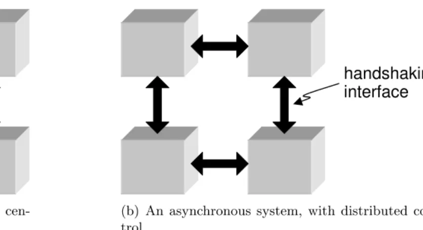
Current trends in micro-electronic design pose a challenge to synchronous systems: (i) high clock speed, (ii) large die area, (iii) handling worst-case delay in deep submicron processes (e.g. 90nmand smaller), and (iv) managing large, complex designs. As a result, an alterna-tive paradigm—asynchronous or “clockless” design—is becoming an increasingly attractive approach because of asynchronous logic’s promise in reversing these negative trends (Berkel et al., 1999). As illustrated in Figure 1.4, instead of using global clocking, an asynchronous system useshandshaking between interacting components to achieve local synchronization.

Asynchronous design has potentially significant energy and performance benefits: lower energy consumption results due to elimination of the power wasted driving the clock, and by limiting switching activity to when and where needed (Berkel et al., 1999). Since local handshaking is used instead of a global clock for synchronization, asynchronous components can gain performance benefits by exploiting the data-dependency of computation completion times (Nowick et al., 1997; Rotem et al., 1999).

Since underlying circuit implementations can largely be decoupled from system level ar-chitecture, the circuit designer is basically free to use exotic techniques, such as clockless logic, while leaving the system architecture unchanged. For example, some modern CPUs, e.g. the Pentium 4, use asynchronous logic to implement their arithmetic units, while still

(26)

clock

(a) A synchronous system, featuring cen-tralized control

handshaking interface

(b) An asynchronous system, with distributed con-trol

Figure 1.4: Synchronous and asynchronous system block diagrams.

realizing a standardized architecture that appears unchanged at a high level. At the extreme, an entire micro-controller has been implemented with asynchronous circuits. This processor is a functional, drop-in replacement for standard synchronous micro-controller (Gageldonk et al., 1998).

1.3.1 Contributions

The work presented in the dissertation involving what we have termed thecircuit axis makes use of asynchronous logic, and increases rendering performance by making graphics hardware more energy efficient, while operating faster for the average case. The dissertation introduces two novel concepts: (i) thecompute-on-demand paradigm, whereby computation at the bit-level is on performed on an as-needed case, and (ii) a novel implementation of the counterflow pipeline architecture. In particular it extends the high capacity (HC) asynchronous pipelining style, which in turn uses dynamic logic, both of which will be briefly described below, and in more detail in Chapter 3.4.

(27)

(a) Rendered frame

0 1 2 3 4 5 6 7 8 9 10 11 12 13 14 15 16 17 18 19 20 21 22 23 0 0.2 0.4 0.6 0.8 1 1.2 1.4 1.6 1.8

2x 10

6

Compute Chain Length

Number of Comparisons

(b) Compute chain length

Figure 1.5: Image (a) shows a frame from Unreal Tournament 2004. The frame requires 6,768,766 comparisons of incoming fragments with the depth buffer. On average, only the 7.3 most significant bits are actually needed to resolve each comparison. Figure (b) shows the distribution of z-comparison compute chain length for the frame shown in (a).

Additionally, I describe an asynchronous Booth multiplier that uses a novel implementa-tion of a counterflow architecture (Sproull et al., 1994) in a single pipeline. In a counterflow architecture, data flows in one direction and control information flows in the opposite di-rection. This counterflow architecture allows for shorter critical paths, and therefore higher operating speed.

While using asynchronous logic in graphics hardware would require dramatic changes at the circuit-level, it would not require (or prevent), changes at the architectural or algorithmic levels.

1.4 Thesis Statement

Using multiple techniques at the circuit, architectural, and algorithmic levels, it is possible to increase the rendering performance of graphics hardware, where rendering performance can be defined as either increasing the energy efficiency of computation, increasing the speed of computation or increasing the visual quality of rendered images.

• Efficient construction of summed-area tables on commodity graphics hardware makes possible dynamic, real-time glossy environmental reflections and dynamic real-time image-based lighting without requiring changes to the underlying architecture.

(28)

• Conditional output streams facilitate an implementation of ray tracing that reduces memory-bandwidth, and allows for high-quality, geometrically correct reflection, refrac-tion, and shadows.

• Asynchronous design techniques, increase energy efficiency, decrease area usage, and increase throughput of basic components used in graphics pipelines.

1.5 Major Contributions

This dissertation presents research at the circuit, architectural, and algorithmic levels that improves the energy efficiency of graphics processors, increases the speed of the computations, and increases the visual quality of rendered images.

My research contributions include along the three axes are:

• Algorithm Axis

– Efficient construction of summed-area tables: I describe a method using graphics hardware to rapidly generate summed-area tables that is efficient enough to allow multiple tables to be generated every frame while maintaining interactive frame rates. Several possible applications of using summed-area tables in interac-tive graphics are presented.

– Offset summed-area tables: I propose a technique that alleviates the precision requirements needed in the construction and use of summed-area tables by off-setting the input image by a constant value. This method improves precision in two ways: (i) there is a 1-bit gain in precision because the sign bit now becomes useful, and (ii) the summed-area function becomes non-monotonic, and therefore the maximum value reached has a relatively lower magnitude, thereby significantly increasing precision by lowering the dynamic range needed to store a summed-area table.

(29)

of a summed-area table — that is efficient enough to allow multiple tables to be generated every frame while maintaining interactive frame rates. I demonstrate using higher order summed-area tables to approximate reflections generated using a Phong BRDF and high dynamic range environment maps.

• Architecture Axis

– Novel ray tracing algorithm using conditional streams: I propose a novel streaming ray casting algorithm. The algorithm uses conditional output streams to reduce memory bandwidth and increase processor utilization when compared to previous methods. The algorithm is able to reduce memory bandwidth by over an order of magnitude compared to the most efficient method presented so far. One possible use for our proposed technique is to implement hybrid rendering algorithms that use standard z-buffering techniques to generate the first hits from the camera view, and then use ray tracing to generate geometrically correct reflections and shadows.

• Circuit Axis

– Compute-on-demand paradigm for asynchronous circuits: I introduce the notion of compute-on-demand as a design principle for fast and energy-efficient graphics hardware. The key idea is to exploit the data-dependent nature of com-putation, and to obtain speed and energy improvements by optimizing the design for the common case, instead of assuming worst-case operation. An asynchronous or clockless circuit style is used to facilitate this paradigm. In particular, only those portions of compute blocks are activated that are actually required for a particular operation, thereby saving energy and reducing critical delays.

– Novel conterflow pipeline approach: I propose a novel implementation of counterflow pipelining which has significant advantages compared with previous implementations; it eliminates the need for complex synchronization and arbitra-tion required between the two distinct data streams in the original counterflow implementation. This feature allows shorter critical paths, and therefore higher

(30)

operating speed. To demonstrate my counterflow methodology, I introduce a novel multiplier organization, in which the data bits flow in one direction, and the Booth commands are piggybacked on the acknowledgments flowing in the opposite direc-tion.

1.6 Dissertation Organization

The remainder of this dissertation is organized as follows:

Chapter 2 discusses increasing rendering performance at the algorithmic level. First, I present background information on summed-area tables, pre-filtering environment maps, and image-based lighting is presented. Next, a method to rapidly construct summed-area tables using graphics hardware is described. Then, a technique to improve the precision requirements of summed-area tables, called offset summed-area tables is presented. Example applications are then described. Next, a method to construct higher-order summed-area tables in real-time is presented. Finally, a dynamic, real-time approximate image-based lighting algorithm.

Chapter 3 describes an architectural extension to commodity graphics processors that would improve processor utilization during execution o conditional operations. The chapter begins by presenting background information on conditional output streams, and GPU-based ray tracing algorithms. Next, as an example of the benefits of conditional streams, a novel ray tracing algorithm is presented. Then the performance of the algorithm is discussed.

Chapter 4 covers techniques used to improve graphics hardware efficiency and performance at the circuit level. It begins with an overview of asynchronous logic, with a particular empha-sis on the High Capacity (HC) pipelining style. Next, a novel asynchronous z-comparator is presented which introduces and illustrates the compute-on-demand paradigm. Then two asyn-chronous Booth multipliers are presented to demonstrate the proposed counterflow pipelining style. Finally, an experiment designed to examine the relationship between pipeline complex-ity and average-case performance is discussed.

(31)

CHAPTER 2

Increasing Rendering Performance Along

the Algorithmic Axis

In this chapter, I present techniques that increase rendering quality on current commodity GPUs. In the next section background information will be presented along with related work. Next, my method for summed-area table construction will be discussed in detail. Additionally, a novel modification to standard summed-area tables, which I have term offset summed-area tables, will be presented. Finally multiple novel algorithms are presented which use summed-area tables to increase the quality of renderings. All of the algorithms presented in this chapter depend on the ability to rapidly generate multiple summed-area tables at interactive rates.

In (Kautz et al., 2000), Kautz et al. presented a method for real-time rendering of glossy reflections for static scenes. They rendered a dual-paraboloid environment map and pre-filtered it in an offline process. Instead of pre-filtering, my algorithm creates a summed-area table for each face of a dual-paraboloid map on the fly, and uses them to filter the environment map at run time. This enables real-time, interactive environmental glossy reflections for dynamic scenes.

2.1 Background

(32)

2.1.1 Reflection and Environment Mapping

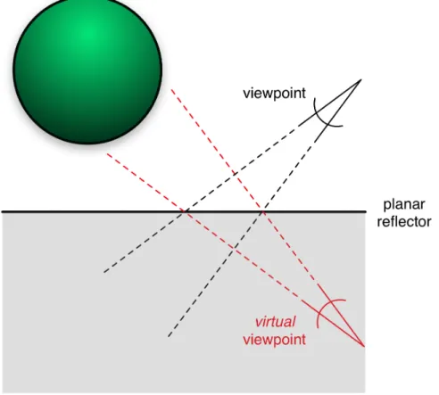
Reflection and environment mapping (Blinn and Newell, 1976) are a set of techniques that are useful for approximating reflection and refraction without having to resort to using ray tracing, which can be expensive or even impossible due to architectural limitations on current graphics hardware.

Figure 2.1: Planar reflection mapping. A virtual camera is placed opposite the planar reflector from the actual camera to generate planar reflections.

2.1.1.1 Planar Reflection Mapping

(33)

physically correct reflections, but suffers from performance issues when there are a large number of planar reflectors, since the scene must be re-rendered separately for each reflector.

2.1.1.2 Cube Mapping

Environment mapping typically assumes that the reflective object, the reflector, is surrounded by a shell, such as a sphere (spherical mapping) or more commonly a cube (cube mapping), and then the environment is projected onto the surrounding shell using the center of the shell as the center of projection. For cube mapping, this process simply requires the scene to be rendered six times, once for each face of the cube. Then during the final rendering pass, the normal to the reflector and the view direction are used to compute a reflection direction which is used to lookup values from thecubemap. Modern graphics chips include support for automatically sampling the correct cube map face given a direction in 3-space.

Most environment mapping techniques make the simplifying assumption that the reflected environment is far from the reflector. When the reflector is relatively close to the environment, or if the center of the reflector is not near the center of the environment map, geometric distortions may be visible since the map has been generated with the center of an enclosing surface as the center of projection.

2.1.1.3 Dual-Paraboloid Mapping

Dual-paraboloid environment mapping (Heidrich and Seidel, 1998) is a technique that stores an environment map in two textures, each of which stores half of the environment as reflected by a parabolic mirror (see Figure 2.2). Typically the alpha channel of each dual-paraboloid map face stores a circular mask that indicates whether a pixel contains relevant data.

A direct mapping from a cube map to a dual-paraboloid map is given by Blythe (Blythe, 1999). The following High Level Shader Language (HLSL) code perfoms the mapping for the front face of the dual-paraboloid map.

samplerCube tCube; // the cubemap to covert to a dual-paraboloid map

(34)

(a) Example dual-paraboloid map. The left column shows thefront map, and the right column shows the back map.

incoming rays

reflected rays (front) reflected

rays (back)

(b) Diagram of a dual-paraboloid map projection. The reflected rays are parallel to each other.

Figure 2.2: Dual-paraboloid maps.

float 4 main (float2 inUV : TEXCOORD0 /* quad texcoord from 0..1 */ )

: COLOR

{

float2 uv = 2.0 * inUV - 1.0; // scale and bias into -1..1 range

float3 dir; // lookup direction for cubemap

// convert front dual-paraboloid face texture coordinate to 3D

// direction

dir.x = 2.0*uv.x;

dir.y = 2.0*uv.y;

dir.z = -1.0 + dot( uv, uv );

dir /= (dot( uv, uv ) + 1.0);

// compute circular mask for alpha channel

(35)

// look up cubemap texture sample and multiply with alpha mask

return float4(texCUBE( texCUBE(tCube, dir).rgb, 1.0) * alpha;

}

A similar shader is used to compute the values for the back map. An alternative to converting 2D texture coordinates to a 3D direction vector in the shader is to pre-compute the conversion and store it in a lookup texture. Then at run-time, an indirect texture lookup is performed during generation of a dual-paraboloid map.

2.1.2 High-Dynamic Range Images

Images in computer graphics are typically represented using low-dynamic range (LDR) values, since the archetypal display can display only a relatively limited dynamic range (the intensity range between black and white). Current commodity LCD displays typically only have a dynamic range on the order of 1000 to 1, whereas real world data will have a dynamic range several orders of magnitude larger.

Instead of using an integer value to represent the intensity of each color channel of an image, high-dynamic range (HDR) images typically use floating point values to represent the intensity of each channel, and allows for more realistic lighting and rendering effects. The availability of commodity graphics processors with single precision floating point native data paths, makes processing HDR data an attractive proposition that can dramatically increase the quality of rendered imagery. Given the limited capabilities of current display technologies, HDR data does have to be mapped to a LDR data via a process calledtone mapping. Tone mapping is a separate topic from the material covered in this chapter, and will not be discussed further in this thesis.

2.1.3 Image-Based Lighting

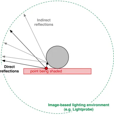
Image-based lighting (IBL), a technique introduced by Debevec (Debevec, 1998; Debevec, 2002), enables synthetic objects to be rendered into real scenes with realistic lighting. This dramatically increases the perceived realism of the synthetic objects. As presented by De-bevec, IBL uses a lightprobe, which is simply an HDR environment map of real world data.

(36)

Lightprobes are typically captured from multiple images taken of a mirrored sphere, which allows radiance data to be captured in all directions. Once a lightprobe is generated, ray trac-ing is used to compute the incident illumination from the image-based lighttrac-ing environment on each of the synthetic surfaces in the rendered scene (see Figure 2.3).

point being shaded

Image-based lighting environment (e.g. Lightprobe)

Direct reflections

Indirect reflections

Figure 2.3: Image based lighting.

Assuming that normalized coordinates are used to access the lightprobe, directions in 3-space can be generated by rotating an normalized vector pointing in the direction of the -z-axis byθ andφ, whereθ and φare given by

u = [−1,1], v= [−1,1] θ = arctan(v/u) φ = π∗p(u2₊_v2₎

Using these relationships, it is a relatively simple task to generate HDR cube and dual-paraboloid environment maps from real world data.

(37)

synthetic object’s BRDF with a lightprobe, thereby approximating the lighting that the synthetic object would have received had it been located at the position where the lightprobe was taken. The use of ambient occlusion (Pharr, 2004) further increases the quality of this approximation.

2.2 Summed-Area Tables

As described in Section 1, summed-area tables enable the rapid calculation of the sum of the pixel values in an arbitrarily sized, axis-aligned rectangle at a fixed computational cost. Figure 1.1 illustrates how a summed-area table is used to compute the sum of the values of pixels spanning a rectangular region. To find the integral of the values in the dark rectangle, we begin with the pre-computed integral from (0,0) to (xR, yT). We subtract the integrals of

the rectangles (0, 0) to (xR, yB) and (0, 0) to (xL, yT). The integral of the hatched box is

then added to compensate for having been subtracted twice.

The average value of a group of pixels can be calculated by dividing the sum by the area. Crow’s technique amounts to convolution of an input image with a box filter. The power lies in the fact that the filter support can be varied at a per pixel level without increasing the cost of the computation. Unfortunately, since the value of the sums (and thus the dynamic range) can get quite large, the table entries require extended precision. The number of bits of precision needed per component is

Ps=log2(w) +log2(h) +Pi

where w and h are the width and height of the input image. Ps is the precision required to

hold values in the summed-area table, andPi is the number of bits of precision of the input.

Thus, a 256x256 texture with 8-bit components would require a summed-area table with 24 bits of storage per component.

Another limitation of Crow’s summed-area table technique is that it is only capable of implementing a simple box filter. This is because only the sum of the input pixels is stored; therefore it is not possible to directly apply a more complex filter by weighting the inputs.

(38)

2.2.1 Higher-Order Summed-Area Tables

In (Heckbert, 1986), Heckbert extended the theory of summed-area tables to handle more complex filter functions. Heckbert made two key observations. The first is that a summed-area table can be viewed as the integral of the input image, and the second that the sample function introduced by Crow was the same as the derivative of the box filter function. By taking advantage of those observations and the following convolution identity

f⊗g=f0n⊗

Z n

g

it is possible to extend summed-area tables to compute higher order filter functions, such as a Bartlett filter, or even a Catmull-Rom spline filter. The process is essentially one of repeated box filtering. Higher order filters approach a Gaussian, and exhibit fewer artifacts such as the blockiness associated with box-filtering.

For instance, Bartlett filtering requires taking the second-order box filter, and weighting it with the following coefficients:

f =

1 −2 −1

−2 4 −2

1 −2 −1

Unfortunately, a direct implementation of the Bartlett filtering example requires 44 bits of precision per component, assuming 8-bits per component and a 256x256 input image.

In general, the precision requirements of Heckbert’s method can be determined as follows:

Ps=n∗(log2(w) +log2(h)) +Pi

wherew and h are the width and height of the input texture, n is the degree of the filter function,Pi is the input image’s precision, andPs is the required precision of thenth-degree

(39)

2.2.2 Related Techniques

Various techniques (Ashikhmin and Ghosh, 2002; Yang and Pollefeys, 2003) have been pre-sented that combine multiple samples from different levels of a mipmap to approximate filter-ing. Ashikhmin and Ghosh approximate simple blurry reflections by using multiple samples from a mipmapped environment map instead of pre-filtering the environment map (Ashikhmin and Ghosh, 2002). By using multiple samples, they are able to approximate various simple BRDFs and blur the environment map on the fly, giving objects the appearance of having glossy BRDFs. Yang and Pollefeys use the same approach to assist in performing depth cor-relation on a pair of stereo images. They take multiple samples from the mip-map and sum them together to approximate a smooth filter functions.

These techniques suffer from several problems. First, a small step in the neighborhood around a pixel does not necessarily introduce new data to the filter; it only changes the weights of the input values. Second, when the inputs do change, a large amount of data changes at the same time, due to the mipmap, which causes noticeable artifacts. Demers et al. (Demers, 2004) added noise in an attempt to make the artifacts less noticeable; although, the visual quality of the resulting images was noticeably reduced.

2.2.3 Efficient Summed-Area Table Generation on GPUs

This section presents one of the major contributions of this thesis. In particular I present a technique to rapidly generate summed area tables on GPUs. In order to efficiently construct summed-area tables, I borrow a technique, called recursive doubling (Dubois and Rodrigue, 1977), often used in high-performance and parallel computing. Using recursive doubling, a parallel gather operation amongst n processors can be performed in onlylog2(n) steps, where

a single step consists of each processor passing its accumulated result to another processor. In a similar manner, the method presented uses the GPU to accumulate results so that only O(log n) passes are needed for summed-area table construction. To simplify the following description, I assume that only two texels, texture elements, can be read per pass. Later in the discussion I explain how to generalize the technique to an arbitrary number of texture reads per pass.

(40)

A B C D A A A A+B A+B A+B B+C A+B+C A+B+C C+D A+B+C+D E D+E A+B+C+D+E A+B+C+D B+C+D+E

Figure 2.4: The recursive doubling algorithm in 1D. On the first pass, the value one element to the left is added to the current value. On the second pass, the value two elements to the left is added the current value. In general, the stride is doubled for each pass. The output is an array whose elements are the sum of all of the elements to the left, computed in O(log n) time.

The algorithm proceeds in two phases: first a horizontal phase, then a vertical phase. During the horizontal phase, results are accumulated along scan lines, and during the vertical phase, results are accumulated along columns of pixels. The horizontal phase consists of n passes, wheren=ceil(log2(image width)), and the vertical phase consists ofmpasses, where m=ceil(log2(image height)).

For each pass a screen-aligned quad is rendered that covers all pixels that do not yet hold their final sum. This prevents pixels that have already computed their final value from wasting precision resources. The input image is stored in a texture named tA. In the first

pass of the horizontal phase two texels are read fromtA: the one corresponding to the pixel

currently being computed and the one to the immediate left. They are added together and stored into texturetB.

For the second pass, the textures are swapped so that data is read from tB and written

totA. Now the fragment program adds the texels corresponding to the one currently being

computed and the one two pixels to the left. tA now holds the sum of four pixels.

The third pass repeats this scheme, now reading fromtAand writing to tB and summing

two texels four pixels apart, resulting in the sum of eight pixels in tB. This progression

(41)

horizontal phase and thus are not covered by the quad rendered in this pass. Next the vertical phase proceeds in an analogous manner. Figure 2.4 shows the horizontal passes needed to construct a summed-area table of a 4x4 image. The following pseudo-code summarizes the algorithm.

tA⇐InputImage

n⇐log2(width)

m⇐log2(height)

// horizontal phase i⇐0

for i < n do

tB[x, y]⇐tA[x, y] +tA[x+ 2i, y]

swap(tA, tB)

i⇐i+ 1 end for

// vertical phase i⇐0

for i < m do

tB[x, y]⇐tA[x, y] +tA[x, y+ 2i]

swap(tA, tB)

i⇐i+ 1 end for

// Texture tA holds the result

In practice, reading more than two texels per fragment, per pass is possible, and this reduces the number of passes required to generate a summed-area table by at least a factor

(42)

of two. The current implementation supports reading 2, 4, 8, or 16 texels per fragment, per pass. This allows trading per-pass complexity with the number of rendering passes required. Adding 16 texels per pass enables us to generate a summed-area table from a 256x256 image in only four passes, two for the horizontal phase, and two for the vertical phase. As shown later, adjusting the per-pass complexity helps in optimizing summed-area generation speed for different input texture sizes. The following is the pseudo-code to generate a summed-area table whenr reads per fragment are possible.

tA⇐InputImage

n⇐logr(width)

m⇐logr(height)

// horizontal phase i⇐0

for i < n do

tB[x, y]⇐tA[x, y]+

tA[x+ 1∗ri, y]+

tA[x+ 2∗ri, y]+ · · ·+

tA[x+r∗ri, y]

swap(tA, tB)

i⇐i+ 1 end for

// vertical phase i⇐0

for i < n do

tB[x, y]⇐tA[x, y]+

(43)

tA[x, y+ 2∗ri]+ · · ·+

tA[x, y+r∗ri]

swap(tA, tB)

i⇐i+ 1 end for

// Texture tA holds the result

Note that near the left and bottom image borders the fragment program will fetch texels outside the image regions. To ensure correct summation of the image pixels, the texture units must be configured to use clamp to border color mode with the border color set to 0. This way texel fetches outside the image boundaries will not affect the sum. Alternatively, it is possible to render a single pixel black border around the input image and configure the texture units to useclamp to edge mode.

The algorithm presented has been implemented in both Direct3D and OpenGL, with simi-lar results. Tables 2.1 and 2.2 summarize the Direct3D results. The OpenGL implementation uses a double buffered pbuffer to mitigate the cost of context switches. Instead of switching context between each pass, the implementation simply swaps the front and back buffers of the pbuffer. This allows us to efficientlyping-pong between two textures as results are accumu-lated. The Direct3D implementation simply uses two different render targets. If implemented at the driver level, similar to the way that automatic mip-map generation is done, the costs of the passes would be reduced even more.

2.2.4 Summed-Area Table Generation Performance

Table 2.1 shows the time required to generate summed-area tables of different sizes on a number of graphics cards using DirectX 9. For each card, and for each of the three input image sizes, we show the shortest time to generate a summed-area table along with the number of texels read per fragment per pass that gives the best result.

(44)

Summed-area table size 256x256 512x512 1024x1024 Radeon

9800 XT1 3.1 ms (8) 14.2 ms (4) 70.1 ms (4) Radeon

X800XT PE1 1.4 ms (8) 7.3 ms (4) 36.2 ms (4) Geforce

6800 Ultra2 4.3 ms (8) 32.4 ms (4) 95.3 ms (4)

Table 2.1: Shortest time to generate summed-area tables of different sizes. The number of samples per pass are given in parentheses. 124−bit f loats 232−bit f loats

Summed-area table size Samples/pass 256x256 512x512 1024x1024

2 2.3 ms 9.9 ms 44.3 ms 4 1.8 ms 7.3 ms 36.2 ms 8 1.4 ms 9.9 ms 45.6 ms 16 2.7 ms 12.4 ms 53.3 ms

Table 2.2: Time to generate summed-area tables of different sizes using different number of samples per pass on a Radeon X800XT Platinum Edition graphics card.

Table 2.2 shows performance based on input size and the number of samples per pass for one of the cards used in the tests. Benchmark results show that finding a good balance between the number of rendering passes and the amount of work performed during each pass is important for the overall performance of summed-area table generation. The optimal tradeoff between the number of passes and per-pass cost is largely dependent on the overhead of switching render targets, which typically causes a pipeline flush, and the design of the texture cache on the target platform.

(45)

2.3 Offset Summed-Area Tables

A key challenge to the usefulness of the summed-area table approach is the loss of numerical precision, which can lead to significant noise in the resultant image. This section first discusses the source of such precision loss and then presents my approach to mitigate this problem (this technique is also described in (Hensley et al., 2005)). Example images are provided that demonstrate how the approach achieves significant reduction in noise: up to 31 dB improvement in signal-to-noise ratios.

2.3.1 Source of Precision Loss

One source of precision loss could be the GPU’s floating-point implementation: Current graphics hardware does not implement IEEE standard 754 floating point but, as shown by Hillesland (Hillesland and Lastra, 2004), current GPU implementations behave reasonably well, so this is not the primary source of numerical error.

The summed-area table approach can exhibit significant noise because certain steps in the algorithm involve computing the difference between two relatively large finite-precision numbers with very close values. This is especially true for pixels in the upper right portion of the image because the monotonically increasing nature of the summed-area function implies that the table values for that region are all quite high.

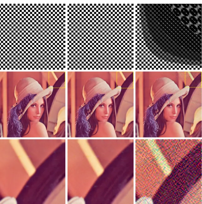
As an example, consider the images of Figure 2.5, which are 256x256 images with 8-bit components. The middle and right columns show the image after being filtered through an ”identity filter,” i.e., a 1-bit filter kernel that is ideally supposed to produce a resultant image that is a replica of the original image. To avoid loss of computational precision, a summed-area table with 24 bits of storage per component per pixel would be sufficient, since the maximum summed-area value at any pixel cannot exceed [256x256]x256. However, the summed-area table used in this example used 16 and 24 bit FP values. 16-bit floating point values are represented with one sign bit, 5 exponent bits, and 10 mantissa bits (s10e5), whereas 24-bit floating point values are represented with one sign bit, seven exponent bits, and 16 mantissa bits (s16e7). As a result, significant noise is seen in the filtered image, with worsening image

(46)

(47)

quality in the direction of increasing xy.

2.3.2 Using Signed-Offset Pixel Representation

Offset summed-area tables simply represent pixel values in the original image as signed floating-point values (e.g., values in the range -0.5 to 0.5), as opposed to the traditional approach that uses unsigned pixel values (from 0.0 to 1.0).

This modification improves precision in two ways: (i) there is a 1-bit gain in precision because the sign bit now becomes useful, and (ii) the summed-area function becomes non-monotonic, and therefore the maximum value reached has a relatively lower magnitude.

I have investigated two distinct methods for converting the original image to a signed-offset representation: (i) centering the pixel values around the 50% gray level, and (ii) centering them around the average image pixel value. The former involves less computational overhead and gives good precision improvement, but the latter provides even better results with modest computational overhead.

Centering around 50% gray level. This method modifies the original image by subtracting 0.5 from the value at every pixel, thereby making the pixel values lie in the -0.5 to 0.5 range. The summed-area table computation proceeds as usual, but with the understanding that the table entry at pixel position (x,y) will now be 0.5xy less than the actual summed-area value. The net impact is a significant gain in precision because the table entries now have significantly lower magnitudes, and therefore computing the differences yields a greater precision result.

Figure 2.5 demonstrates the usefulness of this approach. The first row shows three versions of a checkerboard. The image on the right, reconstructed from a traditional summed-area table, exhibits unacceptable noise throughout much of the image. In contrast, the middle image, generated by our method, shows no visibly perceptible errors.

Centering around image pixel average. While centering pixel values around the 50% gray level proved to be useful, an even better approach is to store offsets from the image’s average pixel value. This is especially true of images such as Lena for which the image average can be quite different from 50% gray. For such images, centering around 50% gray could still result in sizable magnitudes at each pixel position, thereby increasing the probability that the

(48)

(a) Absolute-value of the difference between ground truth and a reconstruction using original summed-area tables.

(b) Absolute-value of the difference between ground truth and a reconstruction using my method (offset summed-area tables).

Figure 2.6: Summed-area table reconstruction error of the inset (bottom row) of Figure 2.5.

summed-area values could appreciably grow in magnitude. Centering the pixel values around the actual image average guarantees that the summed-area value is equal to 0 both at the origin and at the upper right corner (modulo floating-point rounding errors). Figure 2.6 shows the error images between a reconstruction using the original summed-area table algorithm, and the offset summed-area tables method presented in this dissertation.

The computational overhead of this approach is modest as the image average is easily computed in hardware using mip mapping.

2.4 Higher-Order Summed-Area Table Generation

(49)

(a) original image (b) oSAT1 _(box) _(c) _oSAT2 _(Bartlett) _(d) _oSAT3 _(cubic)

Figure 2.7: Comparison of images filtered using repeated offset summed-area tables. Image (a) shows the original input image, half of a dual-paraboloid map computed from the St. Peter’s Basilica light probe (Debevec, 1998). Image (b) is (a) filtered with a box filter using a first order offset summed-area table. Image (c) is (a) filtered with a Bartlett filter using a second order offset summed-area table. Image (d) is (a) filtered with a cubic filter using a third order offset summed-area table. The error in the upper right corner of image (d) is the result of a loss of precision.

boundary pixels. One such padding is to extend the image with black pixels, while arguably, a more reasonable approach is to simply extend the boundary pixels.

There is a simple optimization that traditional approaches use, which is no longer appli-cable when computing higher-order summed-area tables. Traditionally, padding by extending boundary pixel values is actually achieved by re-mapping read accesses to the padded region back to the boundary pixels. Thus, no actual padding is done, but its effect is simulated by ”clamping” the sampling coordinates to the boundary. However, for computing higher order summed-area tables, one cannot use clamping on the first-order summed-area table. In particular, the correct padding is not simply a replication of its boundary values; it is actually the integral of the underlying padded image.

Therefore, for filtering from a second-order summed-area table, instead of clamping, a simple, yet effective, approach is to actually pad the original image, and then do all com-putations on the padded image. This technique ensures that all higher-order summed-area tables are computed accurately, at an increased computational cost. In practice, this does not dramatically affect performance.

(50)

Image 2.7 shows a comparison of filtering a high-dynamic range (HDR) image with a first, a second and a third order summed area table. For the comparison, the first, second, and third order offset summed area tables of the St. Peter’s Basilica Lightprobe were generated using 32-bit floating point arithmetic. For the filtered images, the width of the filter kernel is the same for the different filter orders. The first order filtered image, Figure 2.7(b), clearly shows blocking artifacts from the use of the box filter, while the third order image, Figure 2.7(d) suffers from a loss of precision. The blocking artifacts are greatly exacerbated by the HDR data from the input image, since as soon as bright spot enters the filter kernel, it overwhelms the rest of the data in the filter kernel’s region of support. Figure 2.7(c) shows that filtering with a second order summed-area table offers a reasonable compromise by greatly reducing the blocking artifacts while limiting errors introduced from a loss of precision. Additionally, filtering with a second order summed-area table requires only nine memory accesses, while filtering with a third order summed-area table would require sixteen memory accesses.

2.5 Rendering Glossy Reflections with Summed-Area Tables

Since the technique presented in Section 2.2.2 is efficient enough to generate summed-area tables every frame (less than 2ms for a 256x256 input image on an X800XT PE), their use becomes feasible to generate real-time, interactive effects. This makes summed-area tables an attractive candidate for implementing techniques that approximate dynamic glossy reflections by filtering dynamically generated images.

2.5.1 Glossy Environmental Reflections

(51)

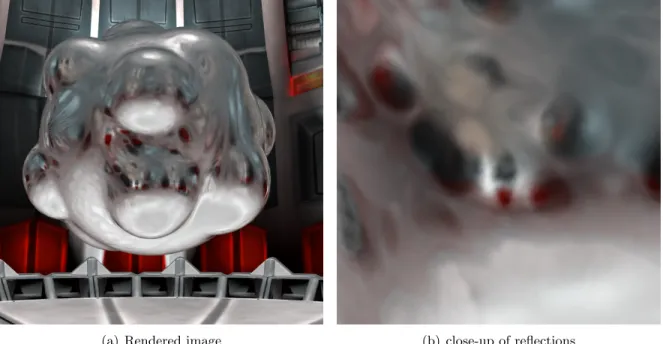
(a) Rendered image (b) close-up of reflections

Figure 2.8: An object rendered with glossy reflections by filtering a dynamic environment map with a spatially varying kernel size. Image (b) shows a close-up of the rendered image, and the spatially varyingglossiness

There are several compelling reasons for using dual-paraboloid environment mapping over the more commonly used cube mapping. First, Kautz et al. showed that when filtering in image space, as opposed to filtering over a solid angle of a hemisphere, a dual-paraboloid environment map has lower error than a cube map or a spherical map. Second, it is only necessary to generate two summed-area tables as opposed to six summed-area tables (one per face of the cube). Finally, for large filters, a dual-paraboloid map requires data from only two textures, whereas it is possible that data might be required from all six faces of a cube map.

A gross approximation to a glossy BRDF is a simple box filter. A single box-filter eval-uation takes four texture reads from the summed-area table. Two evaleval-uations are required in the current implementation when a filter is supported by both the front and the back of a dual-paraboloid map, since at the time of implementation efficientif-else statements were not supported on GPUs. On hardware that has more optimized branching, it is possible to evaluate the filters for both maps only when necessary.

(52)

(a) Rendered image (b) single box filter

Figure 2.9: An object textured using four samples from a pair of summed-area tables generated from an environment map in real-time.

As is common when storing a spherical map in a square texture, our implementation uses the alpha channel to mark the pixels that are in the dual-paraboloid map. A pixel is considered to be in the map if its alpha value is one. The algorithm also uses the alpha value to count the area covered by the filter. After combining the result of the evaluation from the front and back maps, the alpha channel holds the total count of summed texels, which is then used to normalize the filter value.

The basic algorithm for rendering glossy environmental reflections follows.

renderCubeM ap()

generateDualP araboloidM apF romCubeM ap() generateSummedAreaT able(F rontM ap) generateSummedAreaT able(BackM ap) setupT extureCoordinateGeneration() renderScene()

return

renderScene:

(53)

(a) Rendered image (b) stacked filters

Figure 2.10: A set of four box filters stacked to approximate a Phong BRDF.

f ront⇐evaluateSAT(F rontSAT, f ilter size) back⇐evaluateSAT(BackSAT, f ilter size)

// computer filter area

f iltered.alpha⇐f ront.alpha+back.alpha

// combine front and back color result⇐f ront+back

// divide by the area of the filter result⇐result/f iltered.alpha

computeF inalColor(result) end for

While the implementation presented creates a dual-paraboloid map from a cube map, it is possible to directly generate the dual-paraboloid map by using a vertex program to project the scene geometry as done in (Coombe et al., 2004), assuming that the introduced error by this method is acceptable.