MEDIAL/SKELETAL LINKING STRUCTURES
JAMES DAMON1AND ELLEN GASPAROVIC2
Abstract. We introduce a method for modeling a configuration of objects in 2D or 3D images using a mathematical “skeletal linking structure”which will simultaneously capture the individual shape features of the objects and their positional information relative to one another. The objects may either have smooth boundaries and be disjoint from the others or share common portions of their boundaries with other objects in a piecewise smooth manner. These structures include a special class of “Blum medial linking structures”, which are intrinsically associated to the configuration and build upon the Blum medial axes of the individual objects. We give a classification of the properties of Blum linking structures for generic configurations.
The skeletal linking structures add increased flexibility for modeling con-figurations of objects by relaxing the Blum conditions and they extend in a minimal way the individual “skeletal structures”which have been previously used for modeling individual objects and capturing their geometric properties. This allows for the mathematical methods introduced for single objects to be significantly extended to the entire configuration of objects. These methods not only capture the internal shape structures of the individual objects but also the external structure of the neighboring regions of the objects.
In our subsequent second paper [DG2] we use these structures to identify specific external regions which capture positional information about neighbor-ing objects, and we develop numerical measures for closeness of portions of objects and their significance for the configuration. This allows us to use the same mathematical structures to simultaneously analyze both the shape prop-erties of the individual objects and positional propprop-erties of the configuration. This provides a framework for analyzing the statistical properties of collections of similar configurations such as for applications to medical imaging.
1. Introduction
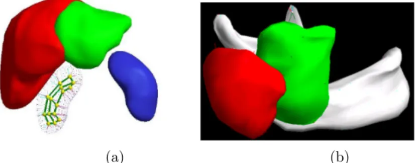
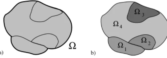
Given a collection of objects, a basic question is how we may simultaneously model both the shapes of the individual objects and their positional information relative to one another. Motivating examples are provided by 2D and 3D medical images, in which we encounter collections of objects which might be organs, glands, arteries, bones, etc (see e.g. Figure 1). A number of researchers have already begun to recognize the importance of using the relative positions of objects in
Key words and phrases. Blum medial axis, skeletal structures, spherical axis, Whitney stratified sets, medial and skeletal linking structures, generic linking properties, model configurations, radial flow, linking flow.
(1) Partially supported by the Simons Foundation grant 230298, the National Science Foundation grant DMS-1105470 and DARPA grant HR0011-09-1-0055. (2) This paper contains work from this author’s Ph. D. dissertation at Univ. of North Carolina.
1
medical images to aid in analyzing physical features for diagnosis and treatment (see especially the work of Stephen Pizer and coworkers in MIDAG at UNC for both time series of a single patient and for populations of patients [LPJ], [GSJ], [JSM], [JPR], [Jg], and [CP]).
In these papers, significant use is made of the mathematical methods which are applied when modeling a single object using a “skeletal structure”[D1], [D3]. Such a structure generally consists of a “skeletal set”, which is a stratified set within the object, together with a multi-valued “radial vector field” from points on the set to the boundary of the object. These form a flexible class of structures obtained by relaxing conditions on Blum medial axes, and these allow one to overcome various shortcomings of the Blum medial axis for modeling purposes. They have played an important role by providing mathematical tools and numerical criteria for fitting discrete deformable templates as models for the individual objects in 3D medial images. These discrete templates, called “M-reps” or in their more general forms “S-reps”, are discrete versions of skeletal structures where the skeletal set is a polyhedral surface with boundary edge, which is topologically a 2-disk (versus the Blum medial axis which would have singularities), and with vectors defined at the vertices. In turn the fitting of the discrete deformable templates to individual objects in the medical images combine the numerical criteria with statistical priors formed from training sets of images. In carrying out the stages of fitting of the models to the objects in the images, the mathematics of skeletal structures is used to guarantee nonsingularity of the models, for the interpolation of the discrete models to yield smooth surfaces, and for ensuring the regularity of resulting object model boundaries.
This approach has been successfully used in numerous cases for modeling objects in medical images, including e.g. the hippocampus, brain ventricles, corpus callo-sum, kidney, liver, and pelvic area involving the prostate, bladder and rectum. For example, many references to papers that use M-reps and S-reps for the analysis of medical images of single objects are given in Chapters 1, 8 and 9 in the book edited and partially written by S. Pizer and K. Siddiqi, see reference [PS].
For certain collection of objects they have have been combined with user chosen, rather adhoc ways, to capture the relative positions between certain objects. While considerable work has been devoted to the application to individual objects, there has not been developed an effective mathematical approach for an entire collection. It is the goal of this paper to describe a mathematical framework for modeling an entire configuration of objects in 2D or 3D, which builds upon the success obtained for individual objects.
We will concentrate on configurations of objects in 2D and 3D images. These can be modeled by a collection of distinct compact regions{Ωi} in R2 or
R3 with
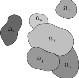
piecewise smooth generic boundaries Bi, where each pair of regions are either dis-joint or only meet along portions of their boundaries in specified generic ways (see e.g. Figure 2). The mathematical results apply more generally to regions in Rn
(see [DG]) even though we concentrate here onR2 andR3.
such information as: the measure of relative closeness of portions of regions, char-acterization of “neighboring regions,”and the “relative significance”of an individual region within the configuration.
Single numerical measures such as the Gromov-Hausdorff distance between ob-jects in such configurations measure overall differences without identifying specific feature variations responsible for the differences. Also invariants that would be ap-propriate for a collection of points fail to incorporate how shape differences between objects contribute to differences in positional structure of such configurations. We will introduce for such configurations “medial and skeletal linking structures,”which allow us to simultaneously capture local and global shape properties of the individ-ual objects and their “positional geometry.”
(a) (b)
Figure 1. Examples of 3-dimensional medical images (obtained
by MIDAG at UNC Chapel Hill) of a collection of physiologi-cal objects which can be modeled by a multi-region configura-tion. a) Prostate, bladder and rectum in pelvic region [CP] and b) mandible, masseter muscle, and parotid gland in throat region (modeled with a skeletal linking structure).
In doing so we have three goals:
(1) minimizing the redundancy of the geometric information provided by the structure while allowing existing mathematical methods for single regions to be extended to configurations;
(2) robustness of the structure’s properties under small perturbations of the object’s shapes and positions in the configuration; and
(3) obtaining quantitative measures from the structure for use in statistical analysis of populations of “configurations of the same type”.
To limit the amount of redundancy, the linking structures extend in a minimal way the notion of a “skeletal structure”for a single compact region Ω with smooth boundary B, developed by the first author [D1] (or see [D3] for regions inR2 and R3). It consists of a pair (M, U), where the “skeletal set”M is a “Whitney stratified
Ω
12
Ω
Ω
3Ω
45
Ω
Ω
6Figure 2. Multi-region configuration inR2.
The added linking structure consists of a multi-valued “linking function”`i de-fined on the skeletal set Mi for each region Ωi and a refinement of the Whitney stratification ofMi on which`i is stratawise smooth. The linking functions`i to-gether with the radial vector fields Ui yield multivalued “linking vector fields”Li, which satisfy certain linking conditions. Even though the structures are defined on the skeletal sets within the regions, the linking vector fields allow us to capture geometric properties of the external region as well.
A special type of skeletal linking structure is a Blum medial linking structure, which builds upon the Blum medial axes of the individual regions. We classify the properties of the Blum linking structures for generic configurations. In obtaining this structure, we identify the regions which remain unlinked and classify their local generic structure of their singular boundaries (which is also the singular set of the convex hull of the configuration). We do this by introducing the spherical axis, which is the analog of the Blum medial axis but for directions inRn, instead
of distances; and it is defined using the family of height functions on the region boundaries.
Just as for skeletal structures for single regions, the skeletal linking structure is a more flexible structure obtained by relaxing a number of the conditions for the Blum linking structure. This allows more flexibility in applying skeletal structures to model objects. Then, as we have already explained, this flexibility is what allows simplified skeletal structures to be used as discrete deformable templates for mod-eling objects [P], overcoming the lack ofC1-stability of the Blum medial axis, and
providing discrete models to which statistical analysis can be applied [P2]. Like-wise the skeletal linking structures have analogous properties, exhibiting stability under C1 perturbations and allowing discrete models for applying statistical anal-ysis. This motivates their potential usefulness for modeling and computer imaging questions for medicine and biology.
[D3] for regions inR2andR3). This includes conditions ensuring the nonsingularity
of a “radial flow”from the skeletal set to the boundary, providing a parametrization of the object interior by the level sets of the flow and implying the smoothness of the boundary [D1, Thm 2.5]. The medial/skeletal linking structure then extends these results to apply to the entire collection of objects, and includes the global geometry of the external region.
In Section 2, we explain what we mean by multi-object configurations and how we mathematically model them using multi-region configurations. Next, in Section 3 we introduce medial/skeletal linking structures for multi-region configurations and give their basic properties. In Section 4, we introduce two versions of a “Blum linking structure”for a general configuration. We first give the generic properties of the Blum medial axis for a region with singular boundary having corners and edge curves (in the case ofR3). The Blum medial axis will now contain the singular
points of the boundaries in its closure and we give an “edge-corner normal form”that the Blum medial axis will exhibit near such singular points. We further give the local form of the stratification of the boundary by points associated to the singular points of the medial axis. It is the generic interplay between these stratifications for adjoining regions and the linking medial axis that gives the generic properties of the linking structure.
For a generic multi-object configuration, which allows shared boundaries that have singular points, we establish the existence of a generic “full Blum linking structure”for the configuration (Theorem 4.13); and later list the generic linking types for the 3D case in Section 6. In the special case where all of the regions are disjoint with smooth generic boundaries, this directly yields a “Blum medial linking structure”(Theorem 4.12). This special case for disjoint regions was obtained in the thesis of the second author [Ga]. In Section 5 we explain how to modify for general configurations the resulting full Blum linking structure near the singular points of the boundaries to obtain a skeletal linking structure. Lastly in Section 7 we explain how the method involving M-reps and S-reps used as deformable templates for single regions can be expanded to obtain deformable templates for an entire configuration based on skeletal linking structures.
In a second paper [DG2], we will use the linking structure we have introduced to determine properties of the “positional geometry”of the configuration. This will include: identifying distinguishing external regions capturing positional geometry; identifying neighboring regions via linking between these regions; introducing and computing numerical invariants of the positional geometry for measures of close-ness and significance of regions in terms of volumetric measurements; computing volumetric invariants (which involve regions outside the configuration) as “skeletal linking integrals”; and combining these results to obtain a tiered graph structure which provides a hierarchical ordering of the regions. This will provide for the comparison and statistical analysis of collections of objects inR2 andR3.
2. Modeling Multi-Object Configurations in R2 andR3
Local Models for Objects at Singular Points on Boundary. We begin by defining what exactly we mean by a “multi-object configuration.”We consider ob-jects which have smooth boundaries if they are separated from the other obob-jects. However, if two objects meet along their boundaries then we allow two different situations, where objects either have flexible boundaries or are rigid. The result-ing possible configurations depend upon which combinations occur. To model such meetings along boundaries, we first describe the form that the object’s boundaries take at the edges of such shared boundary regions.
First, we model the individual objects by compact connected 2D or 3D regions Ω with boundariesBwhich aresmooth manifolds with boundaries and corners. We say that Ω is a manifold with boundaries and corners if each point x∈ Bis either a smooth point of the boundary or is modeled, via a diffeomorphic mapping of a neighborhood of the origin of R2, resp. R3, sending either a closed quadrant
or half space of R2, resp. a closed octant, quarter-space, or half-space of R3 to
a neighborhood of xin Ω, with the boundaries of these regions in R2, resp. R3,
mapping to the boundaryB, see e.g. Figures 3 and 4.
a) b) c) d)
y
x
Figure 3. Model for a (crease) edge in R3 a) and the general
curved edge b); the model for a corner in R2 c) and the general
curved corner d).
y x
z
e) f) g)
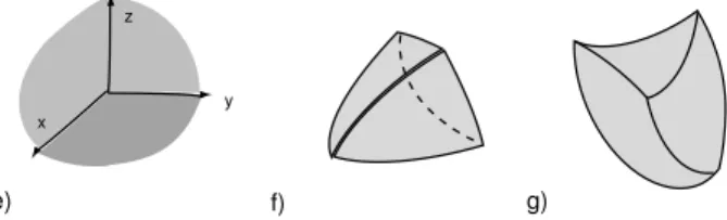
Figure 4. Model for a convex corner in R3 e), and the
corre-sponding curved convex corner f). A concave corner g) may occur where three boundaries of regions which are pairwise mutually ad-joined meet at a point.
Then, the boundaryBis stratified by the corner points, the edge curves (forR3),
and the smooth boundary regions (referred to as regular points of the boundary). The union of the corner points and edge curves (inR3) form the singular points of
the boundary.
common boundary regions, we consider two cases depending on whether the regions are all flexible, or one of them is rigid. In the first case, for 3D objects, we model the edges of regions of common boundary regions by either a)P2; b)P3 in Figure
6. In these figures, one of the regions in the figures may denote the external region complementary to the objects. If one of the regions is rigid then instead the regions meet as in c)Q1 or d)Q2 in Figure 6, where the region with smooth boundary is
the rigid one, and again one of the other regions may denote the external region complementary to the objects. For 2D objects, the local models for meeting are more simply given by either points of typeP2in a) and b) in Figure 5 or typeQ2
in c) and d) in the same figure. We refer to a configuration of regions satisfying the above two conditions regarding their boundary structure and their common boundary regions as satisfying thecombined boundary intersection condition.
a) b) c) d)
Figure 5. Generic local forms for adjoining regions inR2: type
P2consisting of a) two flexible regions meeting and b) three flexible
regions meeting; or typeQ2consisting of c) a flexible region
meet-ing a rigid region and d) two flexible regions meetmeet-ing a rigid region (with the darker rigid region below having the smooth boundary).
(a) (b) (c) (d)
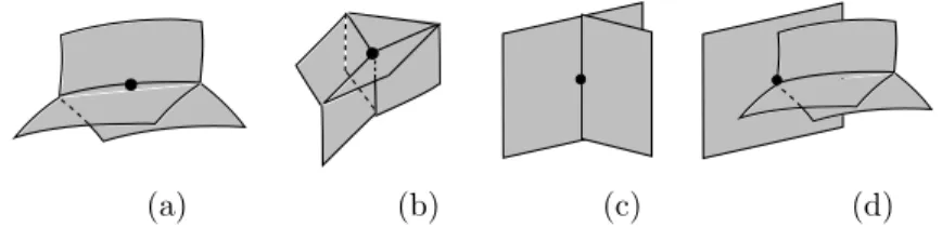
Figure 6. Generic local forms for the boundaries where
adjoin-ing regions inR3 meet: a)P
2 and b)P3 represent the boundaries
of several flexible regions meeting, including possibly the exterior region. Next, c) Q1; and d) Q2 represent the boundaries of
flex-ible region(s) meeting a rigid region (which is to the left and has the smooth boundary). The actual boundaries are diffeomorphic images of these models so the surfaces are in general curved and not planar.
the region below the curve in Figure 5 or to the left of the plane in Figure 6 would represent a rigid region with which one or more flexible regions have contact.
We are going to model a object configuration mathematically with a multi-region configuration, which we define next.
Definition 2.2. A multi-region configuration consists of a collection of compact regions Ωi ⊂R2 or R3, i= 1, ..., m, with smooth boundaries and corners Bi and satisfying the combined boundary intersection condition.
Then, a multi-region configuration will encode as data : i) the topological struc-ture of each region; ii) the regions which share common boundaries and their in-dividual types (flexible or rigid); and iii) the topological structure of the shared boundary regions between two regions. Different regions having the same data will be viewed as having the same configuration type, and changes in the type will be viewed as resulting from a transition of types, see e.g. §5.
The configuration type can change due to: regions that were disjoint coming in contact, or the reverse; boundary regions of contact undergoing topological changes; regions undergoing changes in their topological type (e.g. a hole being created or destroyed); or more subtle positional changes. These are modeled by transitions of configuration type. The generic transitions are the most common ones, but we will not attempt to classify or analyze them here. If we wish to study variations and modifications within a single configuration type, then these can be most effectively described via an embedding mapping of a configuration which we consider next.
The Space of Equivalent Configurations via Mappings of a Model. We introduce amodel configuration∆forΩinRn+1,n= 1,2 which is a configuration
of multi-regions{∆i}satisfying Definition 2.2. Aconfiguration of the same typeas
Ωwill be obtained by an embedding Φ :∆→Rn+1. This means that Φ :∪i∆i→ Rn+1 extends to a smooth embedding in some neighborhood, and it restricts to
diffeomorphisms ∆i 'Ωi for each i, with Bi denoting the boundary of Ωi. Even though the configuration varies with Φ we still use the notationΩfor the resulting (varying) image configuration (with a specific Φ understood). In particular, a configuration of model type ∆ has all of the data of∆ built into it, so different regions Ωi and Ωj will meet along a shared boundary only when the corresponding ∆i and ∆j already do so and otherwise will not meet.
Thespace of configurations of type∆is given by the infinite dimensional space of
embeddings Emb (∆,Rn+1). Then, bygeneric properties of a configurationwe will
mean properties satisfied for an open dense set of embeddings in Emb (∆,Rn+1).
This means that for a configuration that exhibits generic properties, a sufficiently small perturbation will not destroy these properties, and if a configuration does not exhibit these properties, “almost any arbitrarily small perturbation”which is performed will ensure that it does. The generic properties which we give are shown in [DG] to satisfy this property.
We say the regions Ωi and Ωj are adjoining regions if Bi∩ Bj 6= ∅. Also, the
external boundary region of Bi will denote that portion of the boundary which is
shared by the external region. For example, in the multi-region configuration Ω
in Figure 2 the regions Ω1, Ω5, Ω6, are adjoined to Ω2 (and Ω1 and Ω5 with each
Remark 2.3. In the special case of a configuration consisting of disjoint regions with smooth boundaries, each boundary is entirely external. In such a case, we shall see that the geometric relations between the regions are entirely captured via “linking behavior” in the external region.
Because the external region extends indefinitely, we will frequently find for com-putational reasons that it is preferable to have the configuration contained in a “bounded region”. By this we mean an ambient region ˜Ω so that Ωi⊂Ω for each˜ i, then we say thatΩis aconfiguration bounded byΩ. Such a ˜˜ Ω might be a bound-ing box or disk or an intrinsic region containbound-ing the configuration. Then we will also consider bounded configurations either given by an embedding ˜Φ : ˜∆→R2 or
R3, with ˜Φ( ˜∆) denoting ˜Ω, and Φ = ˜Φ|∆; or we fix ˜Ω and consider embeddings
Φ :∆→int ( ˜Ω).
Configurations Allowing Containment of Regions. In our definition of a multi-region configuration, we have explicitly excluded one region being contained in another. However, given a configuration which allows this, we can easily identify such a configuration with the type we have already given. To do so, if one region is contained in another Ωi⊂Ωj, then we may represent Ωj as a union of two regions Ωi and the closure of Ωj\(int (Ωi)∪(Bi∩ Bj)), which we refer to as the region
complementto Ωi in Ωj. By repeating this process a number of times we arrive at
a representation of the configuration as a multi-region configuration in the sense of Definition 2.2. See Figure 7.
Ω
a)Ω
1 2
Ω Ω
3
Ω
4
b)
Figure 7. a) is a configuration of regions contained in a region Ω.
It is equivalent to a multi-region configuration b) which is without inclusion.
3. Skeletal Linking Structures for Multi-Region Configurations in
R2 andR3
The skeletal linking structures for multi-object configurations will be constructed for the multi-region configurations modeling them. They will build upon the skeletal structures for individual regions. We begin by recalling their basic definitions and simplest properties.
Skeletal Structures for Single Regions. We begin by recalling [D1] (or also see [D3]) that a “skeletal structure”(M, U) inRn+1 [D1, Def. 1.13], consists of: a
Whitney stratified set M which satisfies the conditions for being a “skeletal set” [D1, Def. 1.2] and a multivalued “radial vector field” U onM which satisfies the conditions of [D1, Def. 1.5] and the “local initial conditions”[D1, Def. 1.7]. M consists of smooth strata of dimensionn, and the set of singular strataMsing, with ∂M denoting the singular strata whereM is locally a manifold with boundary (for which we use special “boundary coordinates”). For images in R2 and
interested in the cases forn= 1,2; however, the general description is independent of dimension.
Without restating the conditions, we remark that these conditions allow each value of U on a smooth pointx of M to extend to a smooth vector fieldU on a neighborhood of x, and various mathematical constructions on the smooth strata to be extended to the singular strata Msing, see [D1, §2]. Using the multivalued radial vector fieldU, we define a stratified set ˜M, called the “double ofM” and a finite-to-one stratified mappingπ: ˜M →M, see [D1,§3]. Points of ˜M consist of all pairs ˜x= (x, U) whereU is a value of the radial vector field atx, andπ(x, U) =x (see Figure 8). M˜ provides a mathematical method to keep track of both sides of each stratum of M. It also allows multivalued objects on M to be viewed as single-valued objects on ˜M.
a) b) c)
Figure 8. a) illustrates a neighborhood of a point inM and the multivalued vector fields . b) and c) illustrate the two correspond-ing neighborhoods in ˜M.
Likewise we can keep track of the radial lines from each side of M with the space N+ = M˜ ×[0,∞), where for ˜x = (x, U) ∈ M˜, the radial line (actually
a half-line) is parametrized by [0,∞) by c 7→ c ·U. Then, using N+, we can
define the “radial flow”. In a neighborhoodW of a pointx0 ∈M with a smooth
single-valued choice for U, we define a local representation of the radial flow by ψt(x) =x+t·U(x). Together the local definitions yield a global radial flow as a mapping Ψ :N+ →Rn+1defined for ˜x= (x, U) by Ψ(˜x, t) =ψt(x). Beginning with
a skeletal structure (M, U), we can associate a “region” Ω which is the image Ψ(N1),
whereN1= ˜M×[0,1], and its “boundary” B={x+U(x) :x∈M all values of U}.
U
B
M
Ω
Figure 9. Illustrating the radial flow from the skeletal set M,
with the radial vector fieldU, flowing in the region Ω to the bound-aryB, where the level sets are stratified sets forming a fibration of Ω\M.
N1\M˜ and Ω\M; however the level sets of the flow Bt are stratified rather than being smooth. From the radial flow we define the radial map ψ1(x) = x+U(x)
from ˜M toB. We may then relate the boundary and skeletal set via the radial flow and the radial map.
A standard example we consider will be the Blum medial axisM of a region Ω with generic smooth boundaryBand its associated (multivalued) radial vector field U. Then, the associated boundaryBwill be the original boundary of the object.
The compatibility condition involves the compatibility 1-form ηU = dr+ωU,
wherekUk=ris theradial functionandωU(v) =v·uwhereU =r·u, withuthe multivalued unit vector field alongU. Then,ηU is also multivalued with one value for each value ofU. If ηU vanishes on a neighborhood ofxin a smooth region of M, thenU(x) is orthogonal to the boundaryBat the pointψ1(x), and we refer to
U as being “partially Blum”atx. Also, ifηU vanishes onMsing, then the boundary
Bwill be weaklyC1 on the image of the singular set. However, if it does not, then
the boundary will have corners and edges. Hence, skeletal structures can also be used for regions with corners and edges.
Skeletal Linking Structures for Multi-Region Configurations.
We are ready to introduce skeletal linking structures for multi-region configura-tions. These structures will accomplish multiple goals. The most significant are the following.
i) Extend the skeletal structures for the individual regions in a minimal way to obtain a unified structure which also incorporates the positional information of the objects.
ii) For generic configurations of disjoint regions with smooth boundaries, pro-vide a Blum medial linking structure which incorporates the Blum medial axes of the individual objects.
iii) For general multi-region configurations with common boundaries, provide for a modification of the resulting Blum structure to give a skeletal linking structure.
iv) Handle both unbounded and bounded multi-region configurations.
In Part II [DG2] we shall also see that the skeletal linking structure has a second important function allowing us to answer various questions involving the “positional geometry”of the regions in the configuration.
Remark 3.1. Even though a configuration itself is bounded, the complement is unbounded. The properties we shall give will be valid for the unbounded external region; however, for both computational and measurement reasons, it is desirable to consider the configuration as lying in a bounding region. This is the “bounded case”. There are a number of possibilities for such bounding regions: intrinsic bounding region, a bounding box, the convex hull, or a bounded region resulting from imposing a threshold, etc. We shall consider further the relation of these with a skeletal linking structure modeling a given configuration at the end of this section.
We begin by giving versions of the definition for both the bounded and un-bounded cases.
Definition 3.2. A skeletal linking structure for a multi-region configuration{Ωi}
in R2 or
S1) (Mi, Ui) is a skeletal structure for Ωi for each i withUi =ri·ui a scalar multiple ofuia (multivalued) unit vector field andrithe multivalued radial function onMi.
S2) `i is a (multivalued) linking function defined onMi (excluding the strata Mi∞, see L4 below), with one value for each value of Ui, for which the corresponding values satisfy `i ≥ri, and it yields a (multivalued)linking
vector fieldLi=`i·ui .
S3) The canonical stratification of ˜Mi has a stratified refinement Si, which we refer to as thelabeled refinement.
BySibeing a “labeled refinement”of the stratification ˜Miwe mean it is a refinement in the usual sense of stratifications in that each stratum of ˜Mi is a union of strata ofSi; and they are labeled by the linking types which occur on the strata.
In addition, they satisfy the following fourlinking conditions.
Conditions for a skeletal linking structure
L1) `i andLi are continuous where defined onMi and are smooth on strata of
Si.
L2) The “linking flow”(see (3.1) below) obtained by extending the radial flow is nonsingular and for the strata Si j of Si, the images of the linking flow are disjoint and eachWi j ={x+Li(x) :x∈Si j}is smooth.
L3) The strata {Wi j} from the distinct regions either agree or are disjoint and together they form a stratified set M0, which we shall refer to as the
(external) linking axis.
L4) There are strata Mi∞ ⊂ M˜i on which there is no linking so the linking function`i is undefined. On the union of these strata M∞ =∪iMi∞, the global radial flow restricted toN+|M∞is a diffeomorphism with image the complement of the image of the linking flow. In the bounded case, with ˜Ω the enclosing region of the configuration, it is required that the boundary of ˜Ω is transverse to the stratification of M0 and where the linking vector
field extends beyond ˜Ω, it is truncated at the boundary of ˜Ω (this includes M∞).
We denote the region on the boundary corresponding to M∞ byB∞ and that corresponding toMi∞ byBi∞.
Remark 3.3. By property L4), Mi∞ does not exhibit any linking with any other region. We will view it as either theunlinked regionor alternately as being linked to∞, where we may view the linking function as being∞onMi∞. In the bounded case we modify the linking vector field so it is truncated at the boundary of ˜Ω. We can also introduce a “linking vector field on M∞” by extending the radial vector field until it meets the boundary of ˜Ω (see e.g. Figure 12).
For this definition, we must define the “linking flow” which is an extension of the radial flow. We define thelinking flowfromMi by
λi(x, t) = x +χi(x, t)ui(x) where (3.1)
χi(x, t) =
2tri(x) 0≤t≤ 1
2 2(1−t)ri(x) + (2t−1)`i(x) 1
Ω 1
2 Ω
Ω 3 Ω4
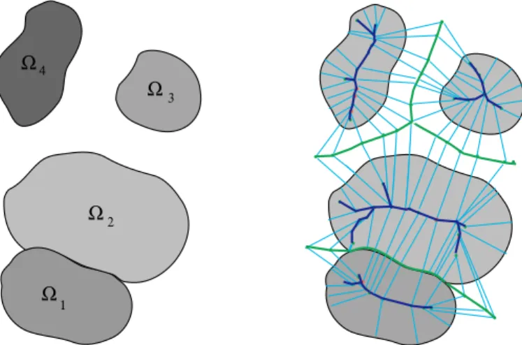
Figure 10. Multi-region configuration in R2 and (a portion of)
the skeletal linking structure for the configuration. Shown are the linking vector fields meeting on the (external) linking axis. The linking flow moves along the lines from the medial axes to meet at the (external) linking axis, which includes the portion of the adjoined boundaries of Ω1 and Ω2.
As with the radial flow it is actually defined from ˜Mi (or ˜Mi\M∞). The combined linking flowsλi from all of theMi will be jointly referred to as the linking flowλ. For fixedtwe will frequently denoteλ(·, t) byλt.
Convention: It is convenient to view the collection of objects for the linking structure as together forming a single object, so we will adopt notation for the entire collection. This includesM for the union of theMi fori >0, and similarly for ˜M. On M (or ˜M) we have the radial vector field U and radial function r formed from the individual Ui and ri, the linking function ` and linking vector fieldLformed from the individual`i andLi; as well as the linking flowλandM∞ already defined.
We see that for 0≤t≤ 1
2 the flow is the radial flow at twice its speed; hence,
the level sets of the linking flow,Bi t, for time 0≤t≤ 1
2 will be those of the radial
flow. For 12 ≤t≤1 the linking flow is from the boundaryBi to the linking strata of the external medial linking axis.
By the linking flow being nonsingularwe mean it is a piecewise smooth home-omorphism, which for each stratum Si j ⊂ M˜i, is smooth and nonsingular on Si j ×
0,12 and either: Si j × 1
2,1
is smooth and nonsingular if Si j is a stra-tum associated to strata inBi0. ForSi j not associated to strata inBi0,`i=ri on Si j, so the linking flow onSi j×12,1is constant as a function oft. That the link-ing flow is nonslink-ingular will follow from the analogue of the conditions given in [D1,
§3] for the nonsingularity of the radial flow. These will be given in Part II [DG2], when we use the linking flow to establish geometric properties of the configuration.
x∈M˜i andx0∈M˜j arelinkedif the linking flows satisfy λi(x,1) =λj(x0,1). This is equivalent to saying that for the values of the linking vector fields Li(x) and Lj(x0), x+Li(x) =x0+Lj(x0). Then, by linking propertyL3), the set of points in ˜Mi and ˜Mj which are linked consist of a union of strata of the stratificationsSi andSj. Furthermore, if the linking flows on strata fromSi k⊂M˜i andSj k0 ⊂M˜j yield the same stratumW ⊂M0, then we refer to the strata as being linked via the
linking stratumW. Then,µi j=λj(·,1)−1◦λi(·,1) defines a diffeomorphiclinking
correspondencebetweenSi k andSj k0.
In Part II [DG2] we will introduce a collection of regions which capture geomet-rically the linking relations between the different regions. For now we concentrate on understanding the types of linking that can occur. There are several possible different kinds of linking. More than two points may be linked at a given point in M0. Of these more than one may be from the same region. If all of the points are
from a single region, then we call the linking self-linking, which occurs at inden-tations of regions. If there is a mixture of self-linking and linking involving other regions then we refer to the linking aspartial linking, see Figure 11.
.
.
.
.
..
.
i)ii)
iii) iv)
v)
Figure 11. Types of linking for multi-region configuration inR2:
The numbers correspond to the generic Blum linking types listed in §4. Also, i) and ii) illustrate linking between two objects; iii) and v) self-linking; and iv) partial linking.
Remark 3.4. If Ωi and Ωj share a common boundary region, then certain strata inMi andMj are linked via points in this boundary region, and for those x∈Mi, `i(x) =ri(x); see Figure 10.
We next consider in more detail the bounded case.
Skeletal Linking Structures in the Bounded Case. For the bounded case we suppose that the configuration lies in the interior of a “bounding region” ˜Ω so that the boundary ∂Ω is transverse to: i) the strata of the external medial axis˜ M0,
hyperplanes for ˜Ω. Hence any line in the tangent plane lies outside int ( ˜Ω). Thus, the radial lines from regions in the configuration will always meet the boundary transversely.
We can alter the linking vector field either by truncating it where it meets the boundary ∂Ω or defining it on˜ M∞ and then refining the stratification so that on appropriate strata the linking vector field ends at ∂Ω. It is now defined on all of˜ Mifor the individual regions Ωi. Because we are either reducing`i, or definingLi onMi∞, the linking flow is still nonsingular.
Thus, we have compact versions of the regions defined for the unbounded case. There are a number of different possibilities for such bounding regions.
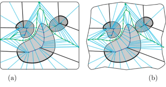
(a) (b)
Figure 12. a) Bounding box with curved corners containing
a configuration of three regions and b) (a priori given) intrinsic
bounding regionfor the same configuration. The linking structure
is either extended to the boundary (in the region bounded by the darker lines on the boundary forMi∞) or truncated at the bound-ary.
Possibilities for a Bounding Region Ω:˜
1) Bounding Box or Bounding Convex Region: The box requires a center and
directions and sizes for the edges of the box. For this, we would need to first normalize the center and directions for the sides of the box and then normalize the sizes of the edges either using a fixed size or one based on feature sizes of the configuration (see e.g. Figure 12 (a)).
2) Convex Hull: The smallest convex region which contains a configuration is
the convex hull of the configuration. For a generic configuration, the convex hull consists of the regionsBi∞together with the truncated envelope of the family of degenerate supporting hyperplanes which meet the configuration with a degenerate tangency or at multiple points. a) of Figure 17 in §4, which is a configuration inR2, the envelope consists of line segments joining
the doubly tangent points corresponding to the points in the spherical axis (b) of Figure 17. In R3, the envelope consists of a triangular portion of
a triply tangent plane, with line segments joining pairs of points with a bitangent supporting plane, and a decreasing family of segments ending at a degenerate point.
3) Intrinsic Bounding Region: If the configuration is naturally contained in
that the extensions of the radial lines intersect ∂Ω transversely, then we˜ can modify the linking structure as in the convex case to have it defined on all of the Mi, and terminating at ∂Ω, if linking has not already occurred˜ (see e.g. Figure 12 (b)).
4) Threshold for Linking: The external region can be bounded by placing
a threshold τ on the `i so that the Li remain in a bounded region. This can be done in two different ways. An absolute thresholdrestricts the ex-ternal regions to those arising from linking vector fields with `i ≤τ; and
a truncated thresholdrestricts to a bounded region formed by replacing `i
by`0i = min{`i, τ}. For the first type, only part of the region would have an external linking neighborhood; while in the second, the entire region would. As for the convex case, since we are replacing `i by smaller values, the linking flow will remain nonsingular. We obtain modified versions of the regions lying in a bounded region.
4. Blum Medial Linking Structure for a Generic Multi-Region
Configuration
In this section we consider two types of linking structures extending the Blum medial axes of the individual objects (i.e. regions). To do so we give a number of results. These include: giving the generic structure of the Blum medial axis for a region with singular boundary allowing corners and edges (inR3); introducing the
“spherical axis”for the configuration, which plays the analogous role for directions as the medial axis plays for distances; and giving the generic properties for the “full Blum medial linking structure”for a general configuration, and its special form in the case of a configuration of disjoint regions with smooth boundaries.
Blum Medial Axis for a Single Region with Generic Singular Boundary.
For a single region we will extend the classification of the generic local structure of the Blum medial axis for regions with smooth boundaries in R2 and
R3 due
to Yomdin [Y], Mather [M], and Giblin-Kimia [GK] (see also [P] and [PS]). For
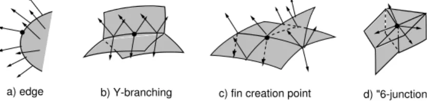
R2 the singular points are either Y-branch points where 3 smooth curves meet
non-tangentially at a point, or end points of a smooth curve. ForR3 the singular
points are either edge points (A3), fin points (A1A3),Y-branch curve points (A31),
or 6-junction points (A41), where six surface segments meet at a point along four Y-branch curves. These are illustrated in Figure 13. The notation A1A3 or Ak1
denotes the singular behavior of the “distance to the boundary”function at the points on the boundary associated to the indicated points on the medial axis.
a) edge b) Y-branching c) fin creation point d) "6-junction"
Figure 13. Generic local medial axis structures inR3: a)A3; b)
Stratification of the Boundary.
The associated points on the boundary form a stratification of the boundary classified by the types of singular points. The boundary classification is shown in [DG, Thm 4.4] to have the generic forms given in Figure 14.
4 1
A
1
A
3
A
3 1
A
A
3 1
A
3
A
Figure 14. Generic local stratification of the boundary for a
region inR3in terms of the type on the medial axis corresponding
to Figure 13: A3andA31are the dimension 1 strata (corresponding
to a) and b)), while the other three are dimension 0. The last two represent A1A3 type from the locations of the A3 point and the
A1 point.
Stratification of the Blum Medial Axis at Singular Boundary Points.
Unlike the case of a region with smooth boundary, the Blum medial axis of a region with singular boundary may extend up to the singular portion. However, in the case of singular points which are either corners or edges (inR3) we can give a
precise characterization of the Blum medial axis near these points.
Definition 4.1. Theedge-corner normal formfor the Blum medial axis of an edge or corner point xin R2 or R3 is the image via a smooth diffeomorphism, sending
the origin to x, of one of the models given in Figure 15. In R2, the model for the
medial axis is given for the corner model by the set of points (x, y) withx=y≥0. In R3, the models are given by either: the set of points (x, y, z) with x= y ≥ 0
for the edge model, or by the set of points (x, y, z) with x, y, z ≥ 0 and one of x=y≥0,x=z≥0, ory=z≥0.
a) b) c)
Figure 15. InR2, a) normal form for the Blum medial axis at a
corner point on the boundary. InR3, b), resp. c) are normal forms
for edge points, resp. corner points. The darker shaded regions represent the Blum medial axis.
We give the following strengthened form for the structure of the Blum medial axis allowing singular points, see [DG, Thm 4.4]
Theorem 4.2(Generic Properties of the Blum Medial Axis). For a generic region
Ω in R2 or
R3 with singular boundary allowing corners and edges (for R3), the
i) it has the same local properties in the interior of the regionint (Ω)as given above for smooth regions (including the local singular structure and proper-ties of the radial vector fields as illustrated for 3D in Figure 13);
ii) the corresponding stratifications of the boundary lie in the smooth strata
(i.e. they miss the edges and corners) and are the same as for the smooth case; and
iii) the closure of the Blum medial axis in the boundary consists of the
singu-lar points of the boundary; at these points, the Blum medial axis has the corresponding edge-corner normal form in Definition 4.1.
Remark 4.3. The Blum medial structure M for a region with boundary and corners contains the singular points of the boundary in its closure, and at such points the radial vector field U = 0. Hence, (M, U) does not define a skeletal structure in the strict sense. However, it can still be used, just as with skeletal structures, to compute the local, relative, and global geometry and topology of both the region and its boundary. Hence, we can view it as a “relaxed skeletal structure,”where “relaxed”means that M includes the singular boundary points and U = 0 on these points. Alternatively, we can modify the Blum medial axis near the singular points of the boundary so it becomes a skeletal structure, see§5.
Spherical Axis of a Configuration. The generic local properties of the Blum medial axis for individual regions described in the last section will also apply to the external linking axis for the Blum linking structure which will be intrinsic for a configuration. There are still two remaining contributions to the linking structure. The one involves identifying the types of linking which may occur generically be-tween different regions. This leads to part of the refinement of the stratification of the Blum medial axes of the individual regions and the external linking axis. The remaining contribution concerns the portions of the Blum medial axes, denoteM∞, and their corresponding boundary pointsB∞ where no linking occurs. These are points on the boundaries where no other regions (or different portions of the same region) would be visible. We characterize the boundary ofB∞using the “spherical axis”and the associated “spherical structure”, which we now proceed to define.
Along with the Blum medial axis, we introduce its analog for directions in place of distances. Directions are given by vectorsv∈Sn, whereSn is the unit sphere in Rn+1. Given such a direction and either a region Ω or a configuration Ω, the
supporting hyperplane in the directionvis given by an equationx·v=c, where all
pointsxof Ω orΩsatisfyx·v≤c(i.e. it is contained in the half-space defined by x·v≤c), with equality at one or more points. The intersection of the supporting hyperplanes defines the convex hull of the region or configuration.
We define the spherical axisZ ⊂Sn of Ω, or the configurationΩ, to consist of directions v ∈ Sn for which the supporting hyperplanes x·v =c for the convex hull of Ω or Ω have two or more tangencies with B or a degenerate tangency, see e.g. Figure 16. If we let τ : B ×Sn →
Rbe defined by τ(x,v) =x·v, then τ is
Theorem 4.4(Generic Properties of the Spherical Axis). For generic regions (with smooth boundaries) or generic configurations, the spherical axis has the following
local structure. InR2,Z consists of a discrete set of points where supporting lines
have two tangent points (see e.g. Figure 17). In R3, it consists of a collection of
branched curves with endpoints. At smooth points of the curves there is a double
tangency of the supporting plane. The branching occurs at Y-branch points which
correspond to triple tangencies. The end points correspond to points where the
height function τ has anA3 singularity. These are illustrated in Figure 16.
a) b) c)
Figure 16. Types of tangencies corresponding to points in the
spherical axis. The tangent planes shown are to points of multiple tangencies (except for the singleA3 point at the left tangency in
c).
Ω 1
Ω 2
Ω 3 Ω
4
Ω 1 Ω
1 Ω
4 Ω
4 Ω
3 Ω 2
a) b) c)
Figure 17. a) Configuration of four regions inR2 with the
bi-tangent supporting lines, and b) the corresponding spherical axis, which consists of the points onS1corresponding to bitangent lines
in a). The regions between points represent subregions of B of unlinked points inB∞. If the same region Ωiis indicated on both sides of a radial line, then inBi is a region involving self-linking. The third figure in c) is a region in R3 with the corresponding
Spherical Structure for a Configuration. Just as for the Blum medial axis, we may associate to the spherical axisZ, both a height functionhand a multivalued vector field V. To do this we need to initialize the origin. Then, the height for a pointu
on the spherical axis, which is a unit vector, defined for a pointx∈ B is just the dot productx·u. Furthermore, there may be multiple points associated tou, all of which lie in the supporting hyperplaneH defined byx·u=h(u), for the maximum valueh=h(u) for B. For each point xi ∈H∩ B, there is a vector V =xi−hu orthogonal to the line spanned byu. This defines a multivalued vector fieldV.
Definition 4.5. The full spherical structure for the spherical axis of the multi-region configuration is the triple (Z, h, V), consisting of the spherical axis Z, the height functionh, and the multivalued vector fieldV. This depends upon the choice of an origin on which all height functions are 0.
From the spherical structure, we can reconstruct the boundary of B∞ by x= V(u) +h(u)u for u ∈ Z and the multiple values of V at u. Here x denotes a collection of points corresponding to the values ofV.
Then, the regions in int (B∞) are the regions in the complement of the boundary of B∞ which have supporting hyperplanes for at least one point in one of the corresponding complementary regions to the spherical axis. If we have in addition the height function for the configuration defined on all ofSn, then we can construct the supporting hyperplanes for all u∈Sn, and the envelope of these hyperplanes yieldsB∞.
Blum Medial Linking Structure. We now consider the analogous Blum medial linking structure for a generic multi-region configuration. First, we note that if the configuration has regions with boundaries and corners, then the Blum medial axes of the individual regions will not define skeletal structures. This is because the Blum medial axis will actually meet the boundary at the edges and corners. However, in the case of disjoint regions {Ωi} in Rn+1 with smooth generic boundaries (which
do not intersect on their boundaries) there is a natural Blum version of a linking structure, which we introduce.
Definition 4.6. Given a multi-region configuration of disjoint regionsΩ ={Ωi} in Rn+1, fori= 1, . . . , m, with smooth generic boundaries (which do not intersect
on their boundaries), aBlum medial linking structureis a skeletal linking structure for which:
B1) theMiare the Blum medial axes of the regions ΩiwithUithe corresponding radial vector fields;
B2) the linking axisM0is the Blum medial axis of the exterior region Ω0 (and
we refer to it as themedial linking axis); and
B3) the Mi∞ are the points in ˜Mi corresponding to points on Bi for which a height function has an absolute maximum (or minimum for the height function for the opposite direction).
Generic Linking Properties.
We consider a generic configuration of regions{Ωi}withBithe boundary of Ωi, andMi the Blum medial axis of Ωi. If each region is generic, then by Theorem 4.2 the Blum medial axis of each region has generic local structure. For 3D, the points on the boundary are of types A3, A31, A41, A3A1 and A1A3, as shown in Figure
14, along with the remaining points of typeA2
1 corresponding to smooth points on
the medial axis. For 2D, there are only isolated points of typeA3, corresponding
to end points of the medial axis andA3
1 points corresponding toY-branch points,
with the remaining points of typeA2 1.
u1
.
Figure 18. Generic linking involves the simultaneous role played by pointsxi∈ Biand their Blum features via the distance function to a pointui of the Blum medial axisMi of the interior region Ωi and that for a pointu0 in the external linking medial axis .
A point ofBi may simultaneously have a role as both a point on the boundary of Ωi and as a point on the boundary of the external region, see Figure 18. As such it has two distinct Blum descriptions, and hence simultaneously belongs to strata on the boundaries corresponding to given Blum behavior exhibited for the individual regions and for the external region. Generic linking between regions for a configuration satisfies special genericity properties which is explained by how these strata intersect.
We consider a collection of smooth boundary pointsS={x1, . . . , xk}withxi∈
Bji associated to pointsui on the medial axes Mji. Suppose theui are linked at
the pointu0on the external medial axisM0. In the generic case, this meansk≤3
forR2 andk≤4 for
R3. We use the notationAαi to denote the Blum type ofxi
for the pointuifor the individual region Ωji and denote the corresponding strata of
the boundary consisting of points of this type by Σαi
Bji. Likewise, we letAβ denote
the Blum type for the pointu0 on the external medial axis, and denote the strata
in the external medial axis by Σ(β)M
0 and the corresponding strata on the boundary
by ΣβB. Then, theBlum linking typeis denoted by (Aβ:Aαi1, . . . , Aαik).
Definition 4.8. The set of pointsS={x1, . . . , xk}as above exhibitsgeneric Blum
linkingof type (Aβ:Aαi1, . . . , Aαik) if:
i) the strata Σ(β)B ⊂ Band Σ(αi)
ii) the images inM0of the strata Σ (β)
B ∩Σ
(αi)
Bji under the linking flow intersect
transversely in the stratum Σ(β)M
0 (see e.g. Figure 19).
For example, generic linking inR2means that zero-dimensional (isolated point)
strata in one region can only be linked to points in the A2
1 strata in another.
Also, inR3a one-dimensional stratum can intersect other one-dimensional stratum
(transversely in a single point) in a boundary Bi and this can then also be linked toA21 strata in another boundary as in Figure 19.
Example 4.9(Generic Linking inR2). There are only five types of generic linking
for configurations inR2(see Figure 11):
i) (A2
1:A21, A21): linking smooth points of two medial axes at a smooth point
of the external medial axis, forming one-dimensional strata;
ii) (A21:A3, A21): linking an end point of one medial axis with a smooth point
of another at an isolated smooth point of the external medial axis, forming a zero-dimensional stratum;
iii) (A21:A31, A21): linking aY-branch point of one medial axis with a smooth
point of another at an isolated smooth point of the external medial axis, forming a zero-dimensional stratum;
iv) (A3
1:A21, A21, A21): linking smooth points of three medial axes at aY branch
point of the external medial axis, forming a zero-dimensional stratum; v) (A3 :A21): a single smooth point of a medial axis is self-linked at an end
point of the external medial axis.
We note that all five types can occur for self-linking; but only the first four can occur for linking between distinct regions; and partial linking can only occur via iv).
By these being the only five generically occurring linking types, we mean that any other possibility, such as e.g. two end points of different regions being linked, may be arranged for a specially constructed configuration; however, almost all slight perturbations of this special configuration will destroy this special linking feature and only involve the five basic types.
For 3D, the situation becomes more complicated and there are seventeen generic linking types listed in Table 1 in§6. However, as explained in§7, by replacing the Blum linking structure with a simpler skeletal linking structure, we can significantly reduce the number of linking types.
Remark 4.10. For a general multi-region configuration, we can substitute in place of Ω0 a region Ωi which has multiple adjoining regions (including possibly the complement Ω0) and the definition of “generic linking”of the adjoining regions
relative to Ωi has the same form as in Definition 4.8. Generically they have the same properties as for Ω0.
Generic Structure forB∞ andM∞.
For a region Ωiof a configuration, the points inMi∞(andBi∞) are not involved in linking; however, they do involve points which have a type Aα based on the
internal medial structure of Ωi. By the generic structure ofMi∞ andBi∞ we are interested in both the generic properties of the stratifications of Bi∞ and Mi∞ resulting from the spherical axis and their relation with the strata Σα
(a)
(a)
(a) (b)
(b) (a)
(a)
(c)
(a) (a)
(a) (a)
(c)
(c)
(c)
(c)
Figure 19. Examples of linking types involving three objects
with a portion of the linking medial axis shown. The points (a) are of linking type (A2
1 : A3, A21); points (b) illustrate linking of
type (A2
1 : A3, A3), and (c) of type (A31 : A3, A21, A21). In the
external linking medial axis is illustrated via the dark curves the 1-dimensional strata of type (A2
1 : A3, A21) with isolated points
either of types (A21:A3, A3) where the 1-dimensional strata cross
or (A31:A3, A21) where the (A 2
1:A3, A21) curve crosses theY-branch
curve of the external linking medial axis.
The interior points of Bi∞ are those points where the supporting hyperplane meets the configuration at a single nondegenerate tangency. In addition, the bound-ary ofBi∞consists of strata Σ(α)∞ corresponding to the strata Σ(α)Z of the spherical axisZ and are of the same dimensions. The strata Σ(α)∞ lie in the smooth strata of theBi.
Definition 4.11. By M∞ andB∞havinggeneric structurewe mean:
1) the spherical axis of the configuration is generic and each Bi∞ has strata with the resulting generic local structure given by Theorem 4.4;
2) the strata of this stratification ofBi∞intersect tranversally the strata Σ
(β)
Bi
for the Blum medial axis of Ωi; and
3) the strata of Mi∞ are the images in ˜Mi of the transverse intersections Σ(α)∞ ∩Σ(β)Bi .
Examples of the generic local structure for the boundary strata of M∞ for a multi-region configuration inR3 are shown in Figure 16: a) of type A21, b) of type
A31, and c) of type A3. The darker curves (including the darker dashed curves)
Existence of a Blum Medial Linking Structure. Before stating the general form of a full Blum linking structure for a general configuration, we first give a special case where the configuration Ω consists of disjoint regions with smooth boundaries. Then, the existence of Blum medial linking structures is guaranteed by the following, which in addition ensures generic linking (see [Ga, Thms 3.4.3 and 3.4.4] and [DG, Thm 4.12]).
Theorem 4.12(Existence of Blum Medial Linking Structure). For a generic
con-figurationΩ={Ωi} in R2 orR3 consisting of disjoint regions with smooth
bound-aries (i.e. they do not intersect on their boundbound-aries), and withΩ contained in the
interior of a given compact region Ω˜,
(1) the configuration has a Blum medial linking structure such that each Mi
(including M0) has generic local properties given by Theorem 4.2;
(2) the linking structure exhibits generic linking as in Definition 4.8;
(3) M∞ and B∞ have generic structure as given in Definition 4.11; and
(4) in the case that Ω˜ is convex, the properties for a linking structure in the
bounded case hold.
This result is a special case of the following general result for a general configu-ration allowing adjoined regions in [DG, Thm 4.13].
Theorem 4.13(Full Blum Linking Structures). A generic multi-region
configura-tionΩ={Ωi} inR2orR3 contained in the interior of a compact regionΩ˜ has the
following generic properties:
i) each Ωi has a Blum medial axisMi exhibiting the generic local properties
at interior pointsof Ωi given by Theorem 4.12;
ii) the external region in Ω˜ has a medial linking axis M0 which exhibits the
generic local Blum properties;
iii) the local structure of the Blum axes Mi (including i = 0) near a
singu-lar boundary point has the local generic edge-corner normal form given by
Definition 4.1;
iv) at a smooth boundary point of a region Ωi of type Qk,k = 2,3, the strata
of Qk-points transversally intersects the strata of Blum type pointsΣ
(α)
Bi ;
v) generic linking occurs between the smooth points of the regions and no linking occurs at edge-corner points; and
vi) Bi∞is contained in the smooth strata of theBi, andBi∞andMi∞exhibit
the generic propertiesgiven in Definition 4.11.
Note: Property v) holds as well for generic linking between adjoining regions of a given region Ωi relative to the region Ωi.
5. Modifying the Full Blum Medial Structure to a Skeletal Linking
Structure
There are two perspectives on this. On the one hand, as mentioned in Remark 4.3, we may view this as a “relaxed form of a skeletal linking structure.”We shall see that from this structure we still obtain all of the local, relative, and global geometry of the individual regions and the positional geometry of the configuration. However, if we consider the stability and deformation properties, such a structure does not behave well.
We describe two approaches to modifying the full Blum linking structure to obtain a skeletal linking structure. One approach is when the configuration with adjoined regions can be viewed as a deformation of a configuration with disjoint regions. The second is to modify the full Blum linking structure by a process of “smoothing the corners”of the regions. We describe each of these.
Example of Evolving Skeletal Linking Structure for Simple Generic Tran-sition. We illustrate the method for a simple generic transition under which two initially disjoint regions Ωi0, i = 1,2, undergo a deformation Ωi t to become
ad-joined at t = t0 and form a common boundary region Zt for t > t0. This is
illustrated in Figure 20.
a) b) c)
Ω'1t
0
Ω'2t
0 Ω'2 0
Ω'1 0
Z t Ω'2t
Ω'1t
Figure 20. The stages for a simple generic transition of two evolving regions Ω0i t becoming adjoined: a) disjoint regions, b) simple tangency at t = t0, and c) regions adjoined along Zt at t > t0.
However, this causes a transition in the full Blum medial linking structure as in changing from a) to b) in Figure 21. There is a discontinuous change in the Blum medial axis somewhat analogous to the introduction of aC1bump in the boundary
of a region which forces the Blum medial axis to introduce a new branch.
An alternate approach is to deform the Blum medial linking structure of the regions before the transition to a skeletal linking structure as the transition occurs and continues for the adjoined regions to evolve from a) to c) in Figure 21. This is achieved by keeping the skeletal axes for each region but altering the lengths of both the radial vectors so they extend to the common boundary and altering the linking vectors to the external linking axis as shown.
This gives a family of skeletal linking structures for the varying configuration
Ω0t ={Ω1t,Ω2t}, which evolve continuously (and stratawise differentiably on the added strataSi t), see Figure 21.
a) b) c)
Z t
M2t
Ω'1t
Ω'2t
Ω'1 0
Ω'2 0
Ω'1t
Ω'2t M1 0
M2 0
M1t M'1t
M' 2t M
0 M
0
Figure 21. Comparison of generic bifurcation of the full Blum
linking structure versus evolution of the retracted skeletal linking structure for two evolving regions Ω0i t becoming generically ad-joined as in Figure 20. Full Blum linking structure bifurcates by adding branches from a) unjoined regions to b) after becoming ad-joined. By contrast, the retracted skeletal linking structure evolves while retaining the structure of the skeletal sets, from a) unjoined regions to c) after being adjoined.
Modifying the Full Blum Linking Structure via Smoothing. A second ap-proach for a configuration with adjoining regions is to modify the full Blum linking structure to a skeletal linking structure. One way to accomplish this is by “smooth-ing of the corners of the regions”in a small neighborhood of the edge/corner set as in Figure 22. The goal is to modify the regions Ωi in a small neighborhoodW of the edge corner points so that the smooth region boundaries are smooth, interior to Ωi and agree with the original boundaries outside of W. This is done in such a way that the radial vector field of the Blum medial axes of the smooth regions can be extended to be transverse to the original boundary and can be extended to meet the external medial axis transversely. These extended vectors are then the linking vectors for a skeletal structure. The details of this can be found in [DG, Chap. 5].
a) b)
M 1
M 2
Ω1
2
Ω M0
Ω1
2
Ω
M1
M 2
M0
Figure 22. An example of a smoothing of a configuration with
6. Classification of Linking Types for Blum Medial Linking Structures in R3
For a generic configurationΩin R3, the Blum medial linking structure exhibits
generic linking properties given in Table 1. We first briefly explain the features of the table. Dimension refers to the dimension inR3 of the strata where the given
linking type occurs. There are three types of linking: 1) linking between points on distinct medial axes; 2) “partial linking” involving more than one point from one medial axis and point(s) from another; and 3) “self-linking” where linking is between points from a single medial axis. “Pure linking type” refers to cases only occurring for self linking. TheA2
1 andA1A3linking can occur for either linking or
self-linking; whileA3
1 andA41 linking can occur for any of the three linking types.
Table 1: Classification of Linking Types for Blum Medial Linking Structures inR3
Linking Type Dimension Description of Linking A21 Linking
i) (A2
1:A21, A21) 2 between 2 smooth points
ii) (A2
1:A31, A21) 1 between a smooth point
and a Y-junction point
iii) (A21:A3, A21) 1 between a smooth point
and an edge point
iv) (A2
1:A3A1, A21) 0 between a fin point
and a smooth point
v) (A2
1:A1A3, A21) 0 between a smooth point
associated to a fin point and another smooth point
vi) (A21:A41, A21) 0 between a smooth point
and a 6-junction point
vii) (A2
1:A31, A31) 0 between 2 Y-junction points
viii) (A2
1:A3, A3) 0 between 2 edge points
ix) (A2
1:A31, A3) 0 between a Y-junction point
and an edge point
A3
1, A41 and A1A3 Linking
x) (A31:A21, A21, A21) 1 between 3 smooth points
xi) (A3
1:A31, A21, A21) 0 between 2 smooth points
and a Y-junction point
xii) (A3
1:A3, A21, A21) 0 between 2 smooth points
and an edge point
Table 1: Classification of Linking Types for Blum Medial Linking Structures inR3
Linking Type Dimension Description of Linking xiv) (A1A3:A21, A21) 0 A1A3 linking between 2
smooth points
Pure Self-Linking
xv) (A3:A21) 1 edge-type self-linking with
a smooth point
xvi) (A3:A31) 0 edge-type self-linking with
a Y-junction point
xvii) (A3:A3) 0 edge-type self-linking with
an edge point
7. Simplifying the Blum Linking Structure for Medical Imaging
For modeling configurations in 2D and 3D medical images, the strategy we pro-pose builds upon that used in modeling single objects using M-reps and S-reps as developed by Pizer and coworkers at UNC MIDAG. The Blum medial axis is re-placed by a simpler skeletal structure where the skeletal set (also called the medial set) is replaced by a surface with boundary diffeomorphic to a 2-dimensional disk, which is modeled by a rectangular grid with a multi-valued vector field at the ver-tices of the grid. Then, the grid together with vectors is the template which is fitted to a specific object in each of a training set of medical images. The size of the grid is experimentally chosen based on the object. The fitting involves an optimization process based on several criteria involving nonsingularity of the structure, regularity of the interpolated vector fields, nonsingularity of the constructed object boundary, and closeness of fit to an expert segmentation of the object. These criteria use in several ways the underlying mathematics of skeletal structures to numerically measure the criterion and contribute to the interpolation technique.
The fitting of the templates provides a discrete set of data for each object in the training set; but the data are points on a product manifold. A form of non-linear PCA is applied to identify the most significant feature directions. Then an iterative process is applied to further refine the fits and ultimately to yield a fit-ting process which is applied to new images using the preceding criteria and the statistical priors. This method provides extremely high quality fit yielding high segmentation accuracy for a number of different cases that have been studied, and led to commercial software for imaging the male pelvic region.