ADVANCED STATISTICAL LEARNING TECHNIQUES FOR HIGH-DIMENSIONAL IMAGING DATA
Leo Yu-Feng Liu
A dissertation submitted to the faculty of the University of North Carolina at Chapel Hill in partial fulfillment of the requirements for the degree of Doctor of
Philosophy in the Department of Statistics and Operations Research.
Chapel Hill 2018
ABSTRACT
LEO YU-FENG LIU: Advanced Statistical Learning Techniques for High-Dimensional Imaging Data
(Under the direction of Yufeng Liu and Hongtu Zhu)
ACKNOWLEDGEMENTS
I would like to express my deepest appreciation to the people who stood by me during my years at UNC. Without their support, this dissertation would not have been completed.
TABLE OF CONTENTS
LIST OF TABLES . . . viii
LIST OF FIGURES . . . x
1 Introduction . . . 1
1.1 Background . . . 1
1.2 Data structure and notation . . . 3
1.3 Image based classification . . . 5
1.3.1 Binary classification . . . 6
1.3.2 Multi-category classification . . . 8
1.4 Image based regression . . . 9
1.5 Deep convolutional neural network model . . . 10
1.6 New contributions and outline . . . 10
2 SMAC: Spatial Multi-category Angle based Classifier for High-dimensional Neu-roimaging Data . . . 12
2.1 Introduction . . . 12
2.2 Methods and materials . . . 15
2.2.1 Data Structure . . . 15
2.2.2 Statistical Classification Framework . . . 15
2.2.2.1 Binary Large-Margin Classifiers . . . 16
2.2.2.2 Multi-category Large-margin Classifiers . . . 17
2.2.3 Spatial Smoothing Regularization . . . 19
2.2.4 Algorithm . . . 21
2.2.5.2 Closed-form solutions for the subproblems . . . 24
2.2.6 Simulation of synthetic data . . . 26
2.2.6.1 Generation of the synthetic data . . . 26
2.2.7 Application: classification of MRI images from ADNI data . . . 28
2.2.7.1 Participants . . . 29
2.2.7.2 Image acquisition and processing . . . 29
2.3 Results . . . 29
2.3.1 Comparison, tuning parameter selection and cross-validation . . . 29
2.3.2 Results from synthetic data analysis . . . 31
2.3.2.1 Cross-validation and tuning results . . . 31
2.3.2.2 Receiver operating characteristic (ROC) analysis and clas-sification accuracy . . . 31
2.3.2.3 Visualization and interpretation of coefficient images . . . 34
2.3.2.4 Model sensitivity on training sample size and noise level . . . 35
2.3.3 Results from ADNI data . . . 38
2.3.3.1 ROC analysis and classification accuracy . . . 38
2.3.3.2 Clinically meaningful coefficient images . . . 39
2.3.4 Computational considerations . . . 42
2.4 Discussion . . . 43
3 SVSIR: Subject Variant Scalar-on-Image Regression . . . 47
3.1 Introduction . . . 47
3.2 Methods and models . . . 50
3.2.1 Data structure and the homogeneous models . . . 50
3.2.2 Subject-specific models . . . 51
3.2.2.1 Homogeneous disease map and its Potts prior . . . 53
3.2.2.2 Individual disease maps . . . 56
3.3 Estimation and prediction . . . 56
3.3.2 Homogeneous region detection . . . 58
3.3.3 Heterogeneous regions assignments . . . 60
3.3.4 Tuning parameter selection . . . 61
3.3.5 Prediction . . . 62
3.4 Theoretical properties . . . 64
3.5 Simulation studies . . . 67
3.6 Real application . . . 74
3.7 Discussion . . . 80
3.8 Proofs . . . 81
3.8.1 Proof of Theorem 1 . . . 81
4 MCNN: Masking Convolutional Neural Network for Image Classification and Regression . . 88
4.1 Introduction . . . 88
4.2 Data structure . . . 90
4.3 Masked convolutional neural network . . . 91
4.3.1 Segmentation module . . . 91
4.3.2 Prediction module . . . 92
4.3.3 Loss functions . . . 92
4.3.4 Implementation . . . 93
4.4 Synthetic simulation experiments . . . 94
4.4.1 Synthetic image regression . . . 94
4.4.2 Noisy MNIST . . . 95
4.5 Real applications . . . 95
4.5.1 Street view house number (SVHN) . . . 96
4.5.2 ADNI MRI classification . . . 97
4.6 Discussion . . . 100
LIST OF TABLES
2.1 List of parameters in Algorithm 1. . . 27 2.2 Demographic information of all subjects in the ADNI data analysis. The
unit for intracranial volume (ICV) is 1,000cm3. The means of age and ICV
are reported, with standard deviations in parentheses. . . 29 2.3 Comparison of the classification results of binary synthetic data.
Classifica-tion accuracy (ACC), true positive rate (TPR), true negative rate (TNR) and area under the ROC curve (AUC) are presented as percentages. Means
from 50 iterations are reported, with standard deviations in parentheses. . . 33 2.4 Comparison of the classification results of multi-category synthetic data.
Classification accuracy (ACC) and area under the ROC curve (AUC1-3) for classes 1, 2 and 3 are presented as percentages. Means from 50 iterations
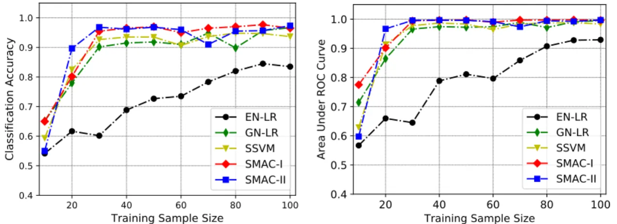
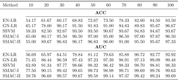
are reported, with standard deviations in parentheses. . . 33 2.5 Sample size sensitivity analysis. Columns represent different training
sam-ple sizes. Classification accuracy (ACC) and area under the ROC curve (AUC) are presented as percentages. The evaluation is based on 600 test
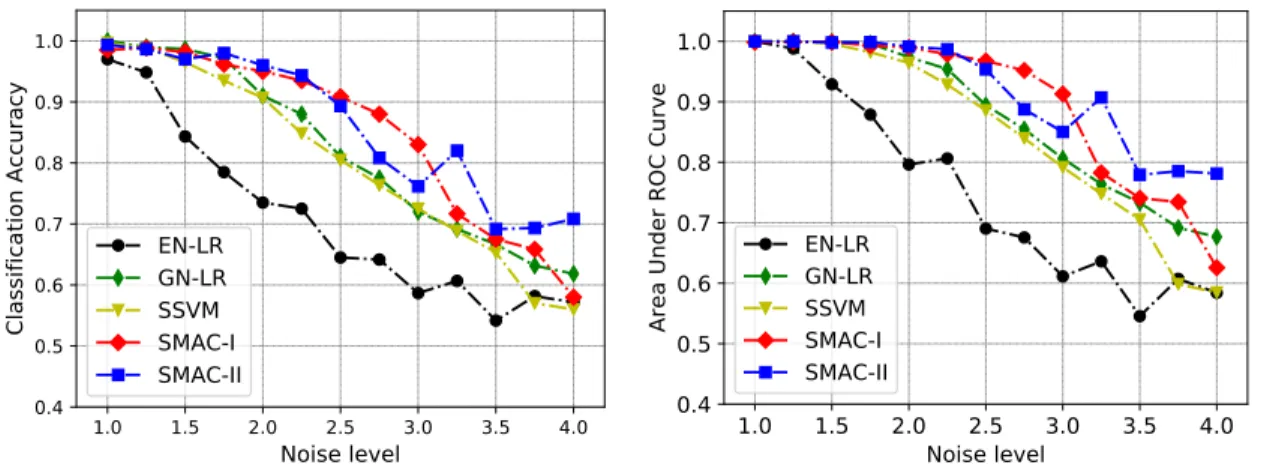
samples. . . 37 2.6 Noise level sensitivity analysis. Columns represent different standard
de-viations of noise. Classification accuracy (ACC) and area under the ROC curve (AUC) are presented as percentages. The evaluation is based on 600
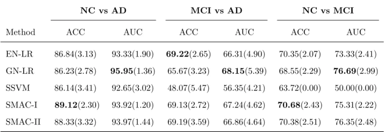
test samples. . . 37 2.7 Comparison of the binary classification results of MRI Data. Classification
accuracy (ACC) and area under the ROC curve (AUC) are presented as percentages. Means from 30 iterations are reported, with standard
devia-tions in parentheses. . . 39 2.8 Comparison of the 3-category classification results of MRI data.
Classi-fication accuracy (ACC) and area under the ROC curve (AUC1-3) with respective reference labels NC, MCI and AD are presented as percentages. Means from 30 iterations are reported, with standard deviations in
paren-theses. . . 39
3.1 The Relative Estimation Error (REE) of the simulation studies. The means
from 50 iterations are reported, with standard deviations in parentheses. . . 70 3.2 The Root Mean Square Prediction Error (RMSPE) of simulation studies.
The means from 50 iterations are reported, with standard deviations in parentheses. . 71 3.3 The demographical information of all subjects in data analysis. The mean
3.4 The mean value of the Root Mean Square Prediction Error (RMSPE) of the ADNI data analysis among 30 random splits. The smallest values are displayed in bold font and underlined, and the second smallest values are
shown in bold font only. . . 77 3.5 The mean value of the correlation between predicted scores and observed
scores of the ADNI data analysis among 30 random splits. The largest values are displayed in bold font and underlined, and the second largest
values are shown in bold font only. . . 77
4.1 Summary of results in the numerical experiments. The mean squared pre-diction errors are reported for the regression problem and the
LIST OF FIGURES
1.1 Plots of three popular modalities of human brain images: Computed To-mography (CT) in the left panel, Magnetic Resonance Imaging (MRI) in the middle panel and Positron Emission Tomography (PET) in the right
panel. All images are displayed in the transverse direction. . . 2 1.2 A typical imaging assisted diagnosis procedure. . . 2
2.1 True signals for two classes of images in Simulation I. The left panel is the true image of class 1: the transparent and yellow regions represent the voxel values of 0 and 1, respectively. The right panel is the true image of
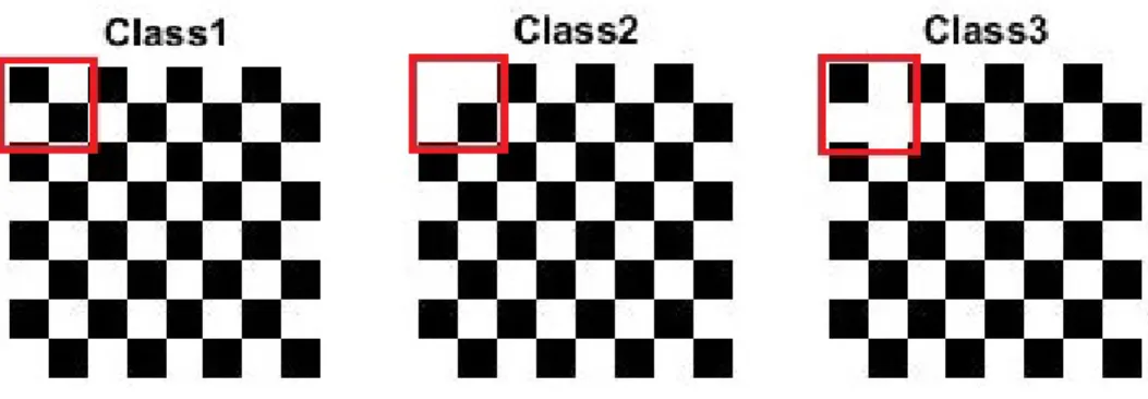
class 2: the transparent, yellow and black regions represent 0,1 and 2, respectively. . . 27 2.2 True signals for three classes of images in Simulation II. The three images
are the top layer (z= 1) of the mean images for classes 1, 2, and 3, respec-tively. White represents the voxel value of 1, and black represents 0. The four layers (z= 1, . . . ,4) of the true image are identical within each class.
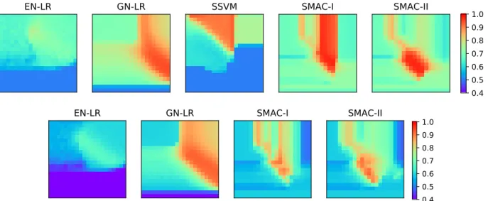
The discriminating regions are marked in red boxes. . . 28 2.3 Validation accuracies for synthetic studies. The top row of 5 panels (from
left to right) respectively correspond to the validation accuracy matrices of EN-LR, GN-LR, SSVM, SMAC-I and SMAC-II for the binary synthetic data. The bottom row of 4 panels (from left to right) respectively corre-spond to the validation accuracy matrices of EN-LR, GN-LR, SMAC-I and SMAC-II for the multi-category synthetic data. Each entry of the matrix is the tuning accuracy for the corresponding combination of λ1 and λ2. The
vertical direction of the matrix represents the value ofλ1, from top to
bot-tom being {0,2−14,2−13, . . . ,25}, and the horizontal direction represents
λ2, from left to right being{0,2−14,2−13, . . . ,25}. . . 32
2.4 Receiver operating characteristic (ROC) analysis for the binary synthetic
data based on 600 test samples. . . 32 2.5 Receiver operating characteristic (ROC) analysis for the multi-category
synthetic data based on 900 test samples. Each panel represents the ROC
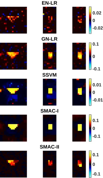
curves evaluated using the “one-versus-the-rest” strategy. . . 33 2.6 Estimated coefficient images obtained from five classification methods in
Simulation I. The 5 panels display the coefficient images of EN-LR, SSVM, GN-LR, SMAC-I and SMAC-II. Each coefficient image is displayed in three respective directions: transverse, coronal and sagittal, from left to right.
2.7 Estimated coefficient images obtained from four classification methods in Simulation II.The top panels are the respective coefficients from EN-LR and GN-LR, and the bottom panels are the coefficients from SMAC-I and SMAC-II. The first two coefficient images (β1 andβ2) of each classifier are displayed. The coefficients from SMAC-I and SMAC-II are obtained using Equation (2.6). All the coefficient images are displayed in the transverse
direction, centered at (16,16,1). . . 36 2.8 Classification results under different training sample sizes. The left panel
displays the classification accuracy and right panel displays the area under
the ROC curve. . . 36 2.9 Classification results under different noise levels. The left panel displays
classification accuracy and the right panel displays the area under the ROC curve. . . . 38 2.10 Estimated coefficient images obtained from five classification methods in
the binary ADNI study. The five plots are the respective coefficient images from EN-LR, GN-LR, SSVM, SMAC-I and SMAC-II. Each coefficient is displayed in the views of coronal, sagittal and transverse planes. The slices
are located at (0,−17,18). . . 40 2.11 Estimated coefficient images obtained from four classification methods in
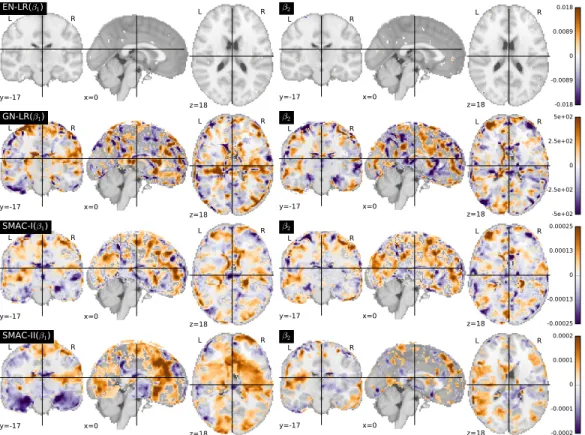
the multi-category ADNI study. The four rows of plots are the respective coefficient images from EN-LR, GN-LR, SMAC-I and SMAC-II. The first two coefficient images (β1 and β2) of each classifier are displayed. The coefficients from SMAC-I and SMAC-II are obtained using Equation (2.6). Each coefficient is displayed in the views of coronal, sagittal and transverse
planes. The slices are located at (0,−17,18). . . 41 2.12 Mean computational time for each method in Simulation I. In each plot,
the vertical direction represents the value of λ1, from top to bottom being
{0,2−14,2−13, . . . ,25}, and the horizontal direction corresponds toλ2, from
left to right being {0,2−14,2−13, . . . , 25}. . . 43
3.1 The brain images of two head & neck patients. The tumors are marked in
the red circles. . . 50 3.2 Example of binary images and their associated local similarity scores. The
top row displays the binary images B1(t) and B2(t), which have exactly
same numbers of 0’s and 1’s. The bottom row displays their associated
local similarity scoressB1(t) and sB2(t). . . 55 3.3 The flow chart of the estimation procedure. . . 61 3.4 An example of the shape-based weights. The left panel is a binary image,
and the right panel is the associated weight matrix, with W1< W2< W3. . . 64 3.5 The plots for the homogeneous coefficient images βin Scenarios 1, 2 and 3
3.6 An example of the synthetic image in the moderate heterogeneity case: the left panel is the coefficient image with 3 non-zero regions. The middle panel is the masking image, indicating that the top two regions are active; and
the right panel is the corresponding covariate image X withRSN R= 0.5. . . 69 3.7 The box plot for the simulation studies. The plots in the top row are
the estimation results for Scenarios 1 to 3 respectively. The plots in the bottom row are the prediction results. The asterisk signs represent the
medians from 50 iterations, and the cross signs denote the 25 and 75 percentiles. . . 72 3.8 The plot of estimated coefficients in Scenario 1 with RSN R= 0.25. The
image on the most left is the true coefficient. The top row is the estimation from ridge regression (RR), Elastic-Net (EN) and Lasso, and the bottom row is the estimation from spatial regularized regression (SREG), functional linear regression (FLR) and the proposed subject variant scalar-on-image regression (SVSIR). The relative estimation error (REE) for these methods
are 0.87, 0.77, 0.78, 0.16, 0.44 and 0.08 respectively. . . 73 3.9 Three typical covariate images from patients with diagnostic labels as NC,
MCI and AD respectively (from top to bottom). . . 75 3.10 The box plot of the Root Mean Square Prediction Error (RMSPE) and the
correlation between predicted scores and observed scores in the ADNI data
analysis among 30 random splits. . . 78 3.11 The plot of the coefficient images from all six methods, with MMSE as responses. . . . 79 3.12 The plot of the coefficient images from all six methods, with ADAS-cog11
as responses. . . 79 3.13 The plot of the coefficient images from all six methods, with ADAS-cog13
as responses. . . 80
4.1 A representative structure of MCNN consisting of the latent binary map-ping module with U-net and a classification network based on VGG (Si-monyan and Zisserman, 2014). Here ⊗ denotes the element-wise product
between the masking matrix and the input image. . . 90 4.2 Estimation results for the synthetic image regression. In each of the two
panels, the image on the left is the original input image. The three images on the top are the estimated masks for Scenario 1-3 respectively. The
images on the bottom are the corresponding masked images. . . 95 4.3 The estimation results for the noisy MNIST experiment. The top row is the
plot of the input images with digits 0 to 9 from left to right. The following
4.4 The estimation results for the SVHN experiment. The left group of images shows two correctly classified images, and the right group corresponds to the misclassified images. Each of the four panels consists of three images:
the original noisy image, the estimated mask and the masked image. . . 97 4.5 Training history of the CNN and MCNN models in the SVHN experiment.
The red and blue lines represent the loss function value of the CNN and MCNN models, respectively. The solid and dashed lines correspond to the
training and validation losses, respectively. . . 97 4.6 Estimation results for the ADNI experiment. The three groups of brain
images respectively show typical samples of Alzheimers disease (AD), mild cognitive impairment (MCI) and healthy status (NC). From top to bottom, each column shows three images: the original image, the estimated mask,
and the masked image. . . 99 4.7 Training history of the CNN and MCNN models in the ADNI experiment.
The red and blue lines represent the loss function values of the CNN and MCNN models, respectively. The solid and dashed lines correspond to the
CHAPTER 1 Introduction
1.1 Background
Neuroimaging technology has been rapidly developed in the past decades. Many imaging tech-niques are widely used to unravel the mystery about the structure and functionality of our neural system, and provide valuable information for the diagnosis and treatment of certain diseases (Giedd et al., 1999; Ogawa et al., 1990; Khoo et al., 1997). For example, advanced imaging techniques, including Computed Tomography (CT), Magnetic Resonance Imaging (MRI) and Positron Emis-sion Tomography (PET) are commonly used both in clinical applications and scientific research to study the functionality of human brains. Figure 1.1 displays some typical brain images, obtained using such techniques. They create images in different ways and measure different aspects of the brain structure and activities. A CT scan uses X-rays taken from different angles to produce cross-sectional images that measure different levels of tissue density inside the brain. MRI is based on the science of nuclear magnetic resonance and uses the gradient field of the radio-frequency signal of hydrogen atoms nuclei to generate brain images. PET images measure the metabolic processes, such as flows of blood to different parts of the brain, via detecting the radioactivity of the injected tracer.
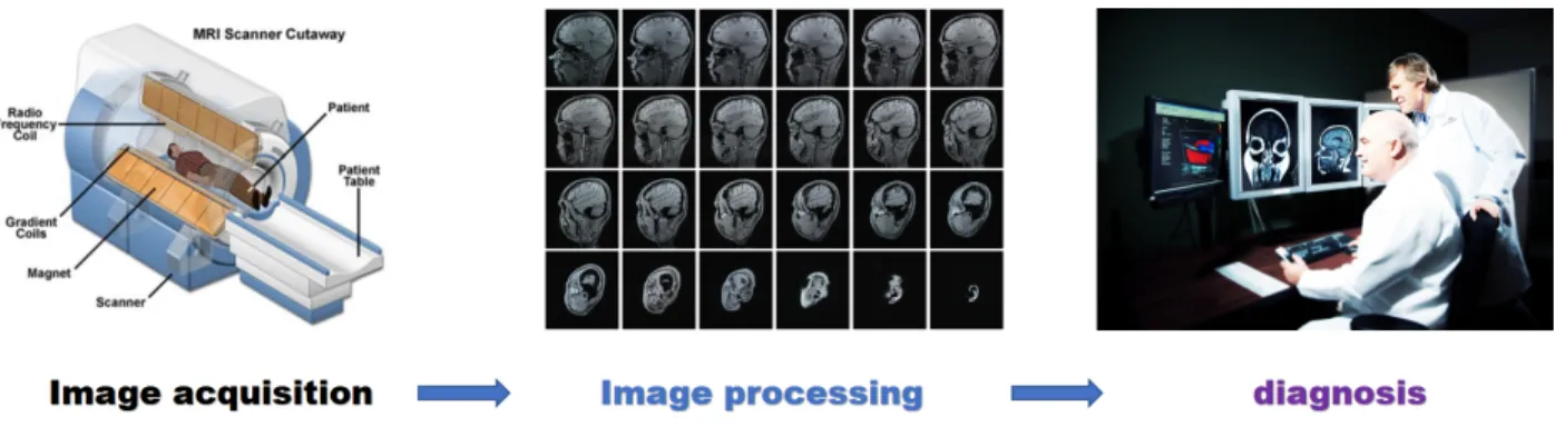
Neuroimaging techniques are widely used for imaging-guided diagnosis procedures. In gen-eral, such procedures include three steps: image acquisition, image processing, and diagnosis. An example of MRI-aided diagnosis is illustrated in Figure 1.2. The imaging-guided diagnosis can significantly improve the accuracy of diagnosed results but requires the expertise of well-trained radiologists, which can be expensive to obtain in practice.
CT MRI PET
Figure 1.1: Plots of three popular modalities of human brain images: Computed Tomography (CT) in
the left panel, Magnetic Resonance Imaging (MRI) in the middle panel and Positron Emission Tomography (PET) in the right panel. All images are displayed in the transverse direction.
medical check-ups in mammography, and in the detection of tumors in the CT scans of lung cancer patients.
The key concept of CAD is to build efficient statistical models, that use medical imaging data to predict important clinical information, and eventually assist radiologists to make diagnosis decisions. There are two types of supervised learning problems in the field of CAD, classification and regression. These two problems can be solved by scalar-on-image models, whose response represents scalar variables and covariate corresponds to imaging data. For classification problems, the scalar responses represent class labels that indicate different stages of disease development, or different clinically meaningful subgroups of patients. For regression, the models are used to predict certain clinical scores as continuous variables, based on image covariates. These clinical scores are usually highly related to the pathology of diseases and can be used as an important guideline to evaluate the effectiveness of treatment plans. For instance, the MiniMental State Examination
(MMSE) score is commonly considered as a benchmark in clinical and research settings to evaluate cognitive impairment and to screen for dementia (Pangman et al., 2000).
For the rest of this chapter, we briefly introduce the framework of scalar-on-image models and review some related works in the literature.
1.2 Data structure and notation
We use bold symbols to represent image variables, such as X and use regular symbols for scalar and other non-image variables, such as y. The notation [n] represents the set{1,2, . . . , n}. The data in the scalar-on-image model are given in pairs of (Xi, yi)’s, where yi denotes the scalar response and Xi represents the corresponding covariate image for thei-th subject.
The image variable X can be viewed as a real-valued function over a bounded image domain, i.e., X = {X(t)∈R; ∀t∈ D}. Here the image domain D denotes a bounded 2-D surface or 3-D
volume, andtis the corresponding location index, which can be a vector of length 2 or 3 according to the dimension of D. The function value X(t) can be the raw image intensity or some other measurement at locationt.
In practice, digital images are often collected with finite resolution, and in this case, the image functions are only evaluated at certain grid points of the whole image domain. Those grid points are usually referred as pixels/voxels. The associated imaging data X are then presented as 2-D matrices or 3-D tensors, with each entry as the pixel/voxel value.
In general, a scalar-on-image model is defined as follows,
yi =f(hXi,βi); fori= 1, . . . , n, (1.1)
whereβdenotes the coefficient image corresponding toXi’s, which can also be treated as a function over the same image domain D. The operation h·,·i denotes the inner product of the two images, which is given by
hXi,βi=
Z
t∈D
Note that, in the discrete setting, the inner product in (1.2) is equivalent to the inner product of two matrices or tensors for 2-D or 3-D images respectively.
According to the definition in Equation (1.1), the scalar-on-image model basically assumes that the yi’s respond to the change of covariate images Xi’ through the inner product of Xi and β, defined in Equation (1.2). This assumption guarantees the coefficient imageβlies on the same space as the covariate images, and thus can incorporate the spatial information of the image domain. We will discuss this property in detail in Section 2.2.3.
In the machine learning literature, the estimation of scalar-on-image models can be summarized in the loss + penalty framework (Hastie et al., 2005). The loss function is used to ensure the goodness-of-fit of the model on the training data, and the penalty term is introduced to avoid over-fitting and encourage some desired structure in the estimated coefficients, such as sparsity. Under this framework, the challenges in estimating the scalar-on-image models mainly arise from the high dimensionality, complex spatial structure, and strong noise in imaging data. High dimensionality is a very common phenomenon in medical imaging data. For example, a typical MRI image of size 256×256×256 corresponds to a variable in the 16,777,216 dimensional space of the statistical model. Due to the high cost of image acquisition facilities, the sample size, i.e., the number of participants in neuroimaging studies is usually very small. This makes the problem fall into the high dimensional low sample size (HDLSS) realm, which was discussed by Hall et al. (2005) in detail. Furthermore, the inherent biological structure of the objects in medical images often present complex spatial correlation and smoothness. Without considering such structure, the models can be hard to interpret and underperformed in terms of prediction. Moreover, the noise of neuroimaging data can be generated in every step of the data acquisition. For example, head motions and machine vibrations in a MRI scan will blur the brain images, and the registration and alignment error in image processing will generate some systematic error of the spatial locations. These noises are spatially correlated and strongly impact the estimation and prediction accuracy, thus require special techniques to deal with.
In the literature, many sparse regularization techniques have been proposed to handle high-dimensional data, including imaging data as a special case. For instance, Tibshirani (1996) intro-duced the Lasso regularization by imposing anL1 norm penalty to high dimensional least squares
groups of correlated predictive variables, this method tends to select only a few variables as rep-resentatives of the groups and ignores the rest. Zou and Hastie (2005) proposed the “Elastic-Net” penalty which regularizes bothL1 andL2 norms of the coefficients. It can avoid the selection issue
with correlated variables by encouraging a grouping effect.
In general, the sparse regularization methods perform the variable estimation and selection simultaneously. They can improve both estimation and prediction performances in a general high dimensional setting. However, for imaging data, the predictive variables are not only sparse, but also spatially clustered in the image domain. Without considering such spatial structures, these regularization methods may underperform when applied in scalar-on-image models. In particular, they tend to delivery coefficient images containing only isolated voxels, which are less clinically meaningful.
To effectively handle imaging data, it is critically important to incorporate its spatial smooth-ness and correlation structure. One efficient approach is to impose the spatial regularization penalty. It has been proven that this approach helps to deliver interpretable coefficient images and improve prediction performance. For instance, Rudin et al. (1992) introduced the total variation penalty that controls the differences between intensities of the adjacent pixels/voxels in the coefficient im-age. Recently, Grosenick et al. (2013) proposed a spatial smoothing penalty named GraphNet by incorporating local graph structure into the Elastic-Net (Zou and Hastie, 2005) regularization. Both methods yield spatially clustered signals in the coefficient images. The total variation penalty yields more clear boundaries between zero and non-zero regions, while GraphNet achieves more spatial smoothness. Despite of progress in these methods, there are still many unsolved problems in the scalar-on-image models. We will discuss some of the unique challenges for image based classifications and regressions separately in the following sections.
1.3 Image based classification
should not only be able to classify patients into clinically meaningful subgroups, but also identify those relevant imaging biomarkers. This is critically important to improve the accuracy of the neuroimaging based computer-aided diagnosis (CAD) and possibly improve treatment plans at an early stage of the diseases.
The mathematical formulation of the image based classification problems can be expressed using the scalar-on-image model in Equation (1.1). The response yi’s are defined as categorical variables, i.e. yi ∈ {1, . . . , K}, representing different groups of subjects. Here K denotes the total number of classes, which is an integer much smaller than the sample size n. The classification model essentially assumes that the pairs of (Xi, yi)’s are drawn from an unknown distribution P(X, y) defined over X × Y, where X denotes the space of all images on the spatial domain D and Y ={1, . . . , K} defines the associated class label space. A classification rulef :X → Y, is a function that maps covariate image X into the class label space {1, . . . , K}. A natural criteria to evaluate a classification rule is to use the corresponding classification error, i.e.,EX,y[I(f(X)6=y)],
whereI(·) represents the indicator function. The optimal classification rule is denoted as the Bayes
rule, which theoretically minimizes the classification error, i.e.,
f∗(X) = argmin f
EX,y[I(f(X)6=y)]
= argmax y P
(y|X).
In practice, since the underlying distribution P(X, y) is unknown, estimation of the classification rule is essentially finding the functions approximating the theoretical Bayes rule.
1.3.1 Binary classification
(QDA) (Hastie et al., 2005) and logistic regression (Cox, 1958; Walker and Duncan, 1967; Hastie et al., 2005). In LDA, the underlying conditional distributions of the covariates,P(X|y = 1) and P(X|y = 2) are commonly assumed to be normally distributed with equal covariance matrices, while in QDA the two classes are allowed to have different covariance structure. Both methods use the maximum likelihood to estimate the conditional distributions, and apply the Bayes’s theorem to predict the class labels. In logistic regression, the class labels are assumed to follow a Bernoulli distributionBer(p). The covariates determine the mean of the distribution through a link function g(p) = hX,βi. The coefficient image β can be obtained using iterative reweighted least squares estimation. These methods work well for low dimensional data, but may underperform when dealing with imaging data, because the estimation procedure can be unstable in the high dimensional setting. Furthermore, the distribution assumptions may not hold for neuroimaging data.
In the past few decades, margin-based methods are getting more and more popular due to their flexibility and improved prediction performance. These methods provide a different view from the likelihood based approaches. Instead of imposing some distributional assumption, these methods directly estimate the classification boundary. In particular, the class labely∈ {1,2}is coded as
Wy =
−1 ify= 1 +1 ify= 2,
and a functionf(·) is introduced, such thatsign(Wyf(X)) can be directly used as the classification rule. Among various margin-based classifiers, perhaps the most well known one is the Support Vector Machines (SVM) (Vapnik, 2013). It estimates the classification rule by solving the following optimization:
min β
n
X
i=1
l(WyihXiβi) +λkβk
2,
(LUM) which covers a range of the margin-based classifiers, including SVM and DWD as special cases. We will revisit LUM in Chapter 2 and discuss the details.
Binary classifiers have been widely used and well studied in the image based classification problems. We refer readers to Rathore et al. (2017) for a comprehensive review of the development on binary classifiers for imaging data in the past thirty years.
1.3.2 Multi-category classification
In contrast to the significant progress in binary image based classification, the developments in category classification are quite limited in the neuroimaging literature. However, multi-category classification is of great importance and deserves more attention. In fact, many neu-rodegenerative diseases, such as Alzheimer’s disease, often have multiple subtypes and transitional stages in their pathophysiological process. Only classifying patients into the disease and health con-trol groups cannot provide sufficient information to characterize the pathophysiological progress. On the other hand, some diseases, such as breast cancer, may have multiple subtypes. Accurately identifying the subtypes of the disease can greatly improve the effect of personalized treatments.
1.4 Image based regression
Image based regression is another important application of the scalar-on-image models. The responses yi’s in such models are continuous and may represent certain pathologically relevant clinical scores. For example, the MiniMental State Examination (MMSE) and Alzheimer’s Disease Assessment Scale Cognitive (ADAS-Cog) scores are widely used to access the cognitive impairment of the patients with Alzheimer’s disease. An effective imaging-based regression model should be able to accurately predict the clinical scores, and efficiently extract the informative imaging biomarkers from the data. This requires a one-to-one correspondence between the location indices in the coefficient images and the covariate images. Thus the linear models are commonly considered and formulated as follows,
yi=β0+hXi,βi+i, (1.3)
wherei’s are the i.i.d. Gaussian noise with mean zeros and the finite varianceσ2.
Note that Model (1.3) can be regarded as a special case of functional linear regressions (FLR) if we treat the images as functions over the image domain. It can also be explained as an extension of the high-dimensional linear models (HDM) if the images are represented as the discrete pixel/voxel values. Both modeling frameworks are extensively studied in the literature among the past decade. We refer readers to the well-known monographs of Ramsay and Silverman (2005), Ferraty and Vieu (2006) and B¨uhlmann and Van De Geer (2011) for details. Despite of the flexibility of the FLR and HDM, the imaging-based regression models still have some unique challenges that cannot be solved by these two frameworks. For example, the HDM assumes the feature indices are interchangeable, but in imaging-based regression these indices are ordered according to the spatial location of the covariate images and thus not interchangeable.
1.5 Deep convolutional neural network model
In the past few years, the deep convolutional neural network (CNN) models have raised huge attention by demonstrating very competitive performance in image related problems, including classification, detection and segmentation. For example, the CNN models have already beat hu-mans in terms of classification accuracy in the MNIST digit recognition (LeCun et al., 1998; Wan et al., 2013) and ImageNet (Deng et al., 2009; He et al., 2016) classification problems. The appli-cation of deep CNN models in neuroimaging problems are also well studied in the recent literature, e.g., (Payan and Montana, 2015) used a 3D convolutional neural network with pre-trained sparse encoders to predict the Alzheimer’s disease using the MRI images; (Wang et al., 2014) applied the extracted features from the CNN models to build a mitosis detector; (Moeskops et al., 2016) and (Zhang et al., 2015) proposed a method using deep CNN models to handle brain segmentation problems.
While the improvement of deep CNN models in image classification and segmentation problems is impressively significant, the model itself works as a “black box” in most cases. Many applications in neuroimaging are still based on existing networks. We will propose a novel convolutional neural network that can handle both the prediction and segmentation tasks simultaneously, and use the estimated segmentation results as a masking image that can indicate the regions in original images that are related to the prediction task.
1.6 New contributions and outline
In this dissertation, I focus on the predictive scalar-on-image models with application in neu-roimaging studies. Both classification and regression problems are investigated. The major con-tributions include extending existing methods to the high dimensional neuroimaging setting and proposing new techniques that overcome some unique challenges in neuroimaging studies.
regularized methods. Both our simulation and application in the Alzheimer’s Disease Neuroimaging Initiative (ADNI) study demonstrate the usefulness of SMAC.
In Chapter 3, we investigate the scalar-on-image regression problems and propose a Subject Variant Scalar-on-Image Regression (SVSIR) model. The SVSIR can yield desired spatially smooth-ing and sparse coefficient images, and incorporate heterogeneity structure among the patients. Ex-tensive numerical studies demonstrate the improvement in terms of both estimation and prediction performance. We also apply the proposed model in the ADNI study, to predict cognitive scores based on MRI data.
CHAPTER 2
SMAC: Spatial Multi-category Angle based Classifier for High-dimensional Neu-roimaging Data
2.1 Introduction
With advances in modern imaging technology, it is becoming increasingly prevalent to collect high-dimensional imaging data (e.g., magnetic resonance imaging [MRI]) in order to extract imaging biomarkers (or features) that are useful for various tasks, including disease detection, diagnosis, prognosis, and treatment, among many others (Chen et al., 1998; Lopez et al., 2009; Ram´ırez et al., 2009). For many diseases, such as Alzheimer’s disease (AD) and breast cancer, it is expected that medical images contain clinically relevant information associated with their pathophysiology. A critical challenge is determining how to build a predictive model (or classifier) that can classify patients into clinically meaningful subgroups according to their imaging data. Such a model may improve the clinical care of these patients and possibly slow their disease progression.
segmen-tation to identify meaningful ROIs in order to extract informative, discriminating and independent features for the classification task.
Image-based analysis, however, uses raw imaging data across all grid points. Two key ad-vantages of using raw imaging data include potential gain in classification accuracy and spatially interpretable coefficient maps of the classifiers in the original image space. The main challenges for image-based analysis include (i) high dimensionality, (ii) complex spatial information and (iii) noisy functional data. For example, a typical T1-weighted MR image of size 256×256×256 will yield a 16,777,216 dimensional space, and due to the inherent biological structure of the brain, these data also have complex spatial correlation and smoothness.
Many methods in the literature apply a pre-screening procedure to reduce the dimensionality of the imaging data, and build classifiers in the reduced image space. For example, Liu et al. (2012) applied the ensemble of multiple classifiers based on randomly selected patches of the MR images, and Hinrichs et al. (2011) built multiple kernel support vector machines based on 2,000 to 250,000 features selected by voxel-wise t-tests. The pre-screening procedure can significantly reduce the computational cost in estimating the classifiers, but potentially loses important predictive information. On the other hand, many regularization techniques have been proposed to directly handle high-dimensional data, including imaging data as a special case (Grosenick et al., 2008, 2009; Yamashita et al., 2008; Van Gerven and Heskes, 2012). For instance, Yamashita et al. (2008) proposed a method by imposing L2 norm regularization to logistic regression for classification of
functional MRI data in various tasks; whereas Casanova et al. (2011) applied elastic-net penalized regression to distinguish between patients with AD versus NCs based on both gray matter and white matter segmentation maps. These regularization methods perform simultaneous estimation of coefficients across all voxels and select the predictive voxels. Since most standard regularization methods do not account for the spatial structure of imaging data, their resulting classifiers usually contain only isolated voxels; thus, it can be difficult to interpret the results. Moreover, standard sparsity penalties, such as L1, can be sub-optimal for the high-dimensional prediction problems
considered here, since the effect of high-dimensional imaging data on certain categories is often spatially clustered and non-sparse.
proposed a spatial smoothing classifier based on the GraphNet penalty. Furthermore, Watanabe et al. (2014) developed a spatial support vector machine (SSVM) classifier based on the fused lasso (FL) and GraphNet penalties. These methods yield meaningful coefficient images and achieve good accuracy for binary neuroimaging classification, but are not directly applicable to multi-category classification problems.
The aim of this chapter is to develop a spatial multi-category angle-based classifier (SMAC) for high-dimensional imaging data. Compared with the existing methods in the literature, three major methodological contributions of this chapter are as follows:
• The proposed SMAC not only utilizes the spatial structure of images, but also extends the angle-based classification framework recently developed by Zhang and Liu (2014) to perform simultaneous multi-category classification of imaging data.
• We use a hybrid of a generalized total variation (TV) penalty (Tibshirani et al., 2005) and a sparse L1 penalty, namely an FL penalty, to identify spatially aggregated clusters that are
important for discriminating different classes. Our methods are able to deliver competitive classification accuracy and interpretable imaging biomarkers.
• We have developed the SMAC package by using both MATLAB and Python and will release it through the website “https://www.nitrc.org/”. Our package includes a graphical user interface that is freely downloadable from the same website. Our SMAC package can handle 1-dimensional (1-D) curves, 2-dimensional (2-D) surfaces, and 3-dimensional (3-D) volumes.
2.2 Methods and materials
2.2.1 Data Structure
One important classification problem in the neuroimaging literature is to predict the disease status of patients based on their neurological images. The class label is denoted by a categorical response variable y, usually taking values of 1,2, . . . , K, indicatingK different classes of interest. The covariate X ={xd:d∈ D} ∈Rp represents the observed imaging data, whereD denotes the spatial space of the image, which can be a 1-D curve, 2-D surface or 3-D volume, anddis a vector of length 1, 2 or 3, indicating the location of the corresponding voxel in the image. Without loss of generality, we focus on 3-D real valued images in this chapter, and usep as the dimension of the imaging data, which equals the total number of voxels in the image.
2.2.2 Statistical Classification Framework
For a K-category classification problem, a statistical classifier builds a map from the covariate space Rp to the category space {1, . . . , K}. Given a new observation X∗, the classifier predicts
the associated class label y∗ as ˆy∗. To build the classifier, many statistical procedures can be fitted into the regularization framework of loss + penalty. A loss function l(·) is introduced to ensure the goodness of fit of the resulting model to the training data. Two groups of loss functions that are commonly used in the literature include likelihood-based and margin-based loss functions. Likelihood-based methods usually impose some assumption of probability distributions on the data and then establish the classification rule by solving some parametric statistical models. Examples of these methods include Fishers linear discriminant analysis (LDA) (Fisher, 1936) and logistic regression (Hastie et al., 2005). In contrast, margin-based methods solve the classification prob-lems without imposing a strong distributional assumption on the data. Specifically, a margin-based method uses a functional margin as the input of the loss functionl(·). The values of the functional margins are directly associated with the accuracy of the class label assignment. For binary clas-sification with the class label Wy ∈ {±1} fory ∈ {1,2}, one can obtain a function f(x) and use
ˆ
indicating the correctness of the classification. Our proposed classifier belongs to margin-based methods.
When dealing with high-dimensional data, a regularization term is usually added to the loss function to prevent the models from over-fitting the training data. The choice of the regularization term is based on prior knowledge of the data structure and the properties of the specific penalty. For instance, theL1 norm penalty can be utilized to learn the sparse structure of data (Tibshirani,
1996), and the L2 type of penalties encourage continuous shrinkage in the estimation (Zou and
Hastie, 2005). To choose the penalty term for handling the neuroimaging data, it is necessary to account for its high dimensionality and complex image structure. A desired penalty should encourage sparsity, while incorporating the spatial structure of the imaging data.
2.2.2.1 Binary Large-Margin Classifiers
Many “off the shelf” classifiers are potential candidates for neuroimaging classification. Exam-ples range from the very classical LDA (Fisher, 1936) and logistic regression (Hastie et al., 2005) to the recent machine learning techniques, such as the support vector machine (Boser et al., 1992) and boosting (Friedman et al., 2000). The choice of the classifier depends on the data structure and the goal of classification. However, there is no clear guideline about which classifier to choose in each complicated case. (Liu et al., 2011) proposed a large-margin unified classifier (LUM), covering a rich family of classification methods, which allows us to tune our loss function within the rich LUM family to obtain a satisfactory solution. In this chapter, we choose a special LUM loss function which has the following form:
l(u) =
1−u, ifu <0; e−u, ifu≥0.
(2.1)
Despite the potential improvement in classification performance when using LUM, this classifier was originally proposed to solve binary classification problems. The extension to multi-category cases requires additional effort. We address this issue in the following section.
2.2.2.2 Multi-category Large-margin Classifiers
To handle multi-category data, one simple approach is to conduct binary classification sequen-tially via the one-versus-one or one-versus-the-rest scheme in order to predict the class labels. These methods have been proven to be suboptimal when there is no dominating class (Liu and Yuan, 2011). Other classifiers solve the classification problem simultaneously by mapping covari-ates to a vector with the length equal to the total number of categories. Such classifiers can be found in (Zhu and Hastie, 2005), (Zhu et al., 2009) and (Liu and Yuan, 2011). A sum-to-zero constraint on the predicted vector is usually applied to achieve desirable theoretical properties, but may increase the complexity of the corresponding optimization. Without this constraint, (Zhang and Liu, 2014) proposed a multi-category angle-based classifier (MAC) that can achieve the Fisher consistency and some other desirable properties.
For a K-category classification problem (K ≥ 2), MAC creates a map from the class labels y∈[K] to the vertices of a regular simplex in the (K−1)-dimensional space, i.e.,
Wy =
(K−1)−1/2ξ, ify= 1; − 1+K1/2
(K−1)3/2ξ+
K K−1
1/2
ey−1, ify∈[K]/1,
(2.2)
where ξ ∈ RK−1 is a vector with all elements being 1, and ey ∈ RK−1 is a vector such that
all elements are 0, except that the y-th component is 1. Note that for K = 2, it reduces to the traditional binary classification with labels Wy ∈ {±1}. Due to the property of the regular simplexes, the angles between any two projected class labels are equal, i.e., ∠(Wy, Wy0) = CK for
all y6=y0.
Wy fory ∈[K] to determine the prediction rule, i.e.,
ˆ
y= argmin y ∠
(Wy, f(X)).
According to the “law of cosine”, this is equivalent to
ˆ
y= argmax y
hWy, f(X)i, (2.3)
where h·,·i denotes the inner product of two vectors. The inner product essentially plays the role of the functional margin in MAC, and the empirical risk minimization (ERM) is, therefore defined as follows:
min f∈F
( n
X
i=1
l(hWyi, f(Xi)i) +λJ(f)
)
, (2.4)
wherel(·) is the margin-based loss function defined by equation (2.1) andJ(f) denotes the penalty term with the tuning parameter λ, which controls the strength of regularization.
Considering the specialty of voxel-based neuroimaging classification, we narrow the function space F to linear functions, so that the coefficients of f(·) are voxel-wisely matched with the structure of the image covariateX, i.e.,
f(X) = (f1(X), f2(X), . . . , fK−1(X))T ,
fj(X) =βj,0+x1βj,1+. . .+xpβj,p forj∈[K−1]. (2.5)
Notice that βj = (βj,1, . . . , βj,p)T has a one-to-one correspondence with the imaging data X = (x1, . . . , xp)T. Thus, it can be also defined in the original image space of the covariates. In this case, we denoteβj as the coefficient image of the fitted classifier.
For a K-category classification problem, we have K−1 coefficient images. In order to match the coefficient images with the K class labels, we denote the reconstructed coefficient images β∗y, y∈[K] of the same dimension of βj as follows,
β∗y = K−1
X
j=1
whereWy,j is the j-th element of the project class label Wy in Equation (2.2) and “·” denotes the element-wise product.
Note that β∗y has the one-to-one correspondence with the class label y. Additionally, since
PK
y=1Wy = 0 according to Equation (2.2), we have the sum-to-zero constraint on β ∗
y’s as well, i.e.,
PK
k=1β ∗
y = 0. These properties ensure that the reconstructed coefficient images are comparable with the coefficient images obtained from other linear classification models with the sum-to-zero constraint, such as logistic regression.
2.2.3 Spatial Smoothing Regularization
The penalty term J(f) in problem (2.4) not only plays an important role of preventing the resulting classifier from over-fitting, but also helps to achieve some desired structure in the coefficient images. For image classification, unpenalized estimation often yields dense coefficients, but requires additional thresholding (or feature selection) to identify meaningful biomarkers. In contrast, the use of sparse penalties alone, such as lasso and the elastic net, leads to coefficient images with isolated voxels, which can be difficult to interpret. The use of spatial smoothing penalties not only captures the spatial smoothness in the image space, but also yields biologically interpretable coefficient images. For instance, Grosenick et al. (2013) proposed a spatial smoothing penalty, GraphNet, that incorporates the spatial structure in the elastic net penalization. However, the GraphNet penalty yields global smoothness in coefficient images, so it may be suboptimal in preserving sharp edges.
We introduce the generalized FL penalty (Tibshirani, 2011) to capture the spatial structure of imaging data. For an image I = {I(d) ∈R :d∈ D}, the discrete image intensities are evaluated at grid points d = (d1, d2, d3)T ∈ R3 in a compact setD. The FL penalty is a weighted mixture
of the L1 and TV penalty on the image intensities. The L1 penalty encourages both shrinkage
and sparseness (Tibshirani, 1996); whereas the TV penalty regularizes the differences between the consecutive elements in the estimation. We denote the latter as the TV-I penalty. Its discrete formulation is defined as follows:
TV-I(I) = D1
X
d1=1
D2
X
d2=1
D3
X
d3=1
where|| · ||1 denotes the L1 norm,D1,D2 andD3 respectively represent the total number of voxels
along each dimension, and ∇ denotes the discrete differential operator such that ∇Id1,d2,d3 = (∇1Id1,d2,d3,∇2Id1,d2,d3,∇3Id1,d2,d3)T. Moreover,∇1Id1,d2,d3 is defined as
∇1Id1,d2,d3 =
Id1,d2,d3 −Id1+1,d2,d3 if 1≤d1 ≤D1−1,
0 ifd1 =D1,
and ∇2Id1,d2,d3 and ∇3Id1,d2,d3 can be similarly defined.
The TV-I penalty penalizes the discrete gradient of the image functionI(·). It encourages the spatial smoothness of I(·), while capturing its sharp edges. This property allows us to efficiently detect important blobs. However, in some cases, the TV-I penalty tends to yield images with block-wise constant blobs (Rudin et al., 1992), which might erase too many details. For this reason, we introduce the second-order TV penalty, denoted TV-II, which can capture blobs with a continuous change of intensity by imposing the regularization on the Hessian matrix of I(·), which encourages the gradual fade ofI(·) in the space. The discrete formulation of TV-II is defined as follows:
TV-II(I) = D1−2
X
d1=1
D2−2 X
d2=1
D3−2 X
d3=1
||H(Id1,d2,d3)||1, (2.8)
whereH(Id1,d2,d3) = (∇m(∇m0(Id1,d2,d3)))
1≤m,m0≤3 and || · ||1 denotes the entry-wise L1 norm of a
matrix.
Note that the calculation of both gradient and Hessian operators can be represented as matrix multiplication on the vectorized images. In particular, the TV-I(I) in (2.7) can be represented as
TV-I(I) =||D×I||1,
where D denotes the discrete derivative operator that contains the differencing operation along each of the 3 dimensions of the image domain.
Similarly, the TV-II penalty can be represented as
whereDII = diag{D,D,D}is a diagonal block matrix, with 3 copies of matrixDrepresenting the operations along each dimension.
For problem (2.4), we haveK−1 coefficient images for aK category classification problem and can denote β= (β1, . . . ,βK−1)T as the vector of all the image coefficients, as denoted in equation
(2.5). The associated TV-I penalty is defined as
TV-I(β) = K−1
X
k=1
TV-I(βk) = K−1
X
k=1
||D×βk||1 =||CIβ||1,
whereCI = [D, . . . ,D] isK−1 copies of the operator D. Similarly, we can define
TV-II(β) =||CIIβ||1,
whereCII = [DIID, . . . ,DIID] is K−1 copies of the matrix DIID. Finally, the EMR problem in (2.4) can be reformulated as follows:
min β∈R(K−1)(p+1)
( n
X
i=1
l(hWyi, f(Xi)i) + FL(β) )
, (2.9)
where l(·) is the loss function in (2.1), f(·) is a system of linear functions defined in (2.5), and FL(β) = λ1||β||1+λ2||Cβ||1 defines the FL penalty, in which λ1 and λ2 are two non-negative
tuning parameters andC=CI for TV-I orCII for TV-II.
2.2.4 Algorithm
2.2.5 Alternative Direction Method of Multipliers
The ADMM algorithm (Boyd et al., 2011; Mota et al., 2011) was developed to handle large-scale convex optimization problems with the following separable and constrained structure:
min
X,Y
g1(X) +g2(Y) subject to A1X+A2Y= 0, (2.10)
where X ∈ Rp and Y ∈ Rq are unknown parameters, g1(X) and g2(Y) are two closed convex
functions, andA1 ∈Rm×p and A2 ∈Rm×q represent mlinear constraints onXand Y, respectively.
ADMM solves (2.10) by breaking them into smaller and simpler subproblems and solving them alternatively. Specifically, for the t+ 1 iteration,
Xt+1 = argmin
X
n
g1(X) +ρ
2||A1X+A2Y
t+ut||2 2 o
,
Yt+1 = argmin
Y
n
g2(Y) +ρ
2||A1X t+1+
A2Y+ut||22 o
,
ut+1 =A1Xt+1+A2Yt+1+ut,
where ρ denotes the augmented Lagrangian parameter, u is a vector of dual variables, and || · ||2 denotes theL2 Euclidean norm. The choice ofρaffects the convergence rate of the algorithm (Boyd
et al., 2011), and remains an open question in the literature. We implement our algorithm with ρ= 1, but it can be tuned in practice.
2.2.5.1 Reformulation of ERM
We first reformulate the ERM (2.9) so that the ADMM algorithm can be applied smoothly. Note that the evaluation of the functional margins hWyi, f(Xi)i consists of only linear operations. We construct a big matrixA, such that the inner product can be simplified as one matrix multiplication, i.e.,
hWyi, f(Xi)i= K−1
X
k=1
Wyi,k(hXi,βki+βk,0) =Ai,.β fori∈[n], (2.11)
The penalty term in (2.9) consists of a sum of two L1 norms of vectors, and thus can be
simplified as
||Bβ||1=λ1||β||1+λ2||Cβ||1,
where BT = [λ
1I, λ2CT]. With a little bit of adjustment to the notations, we use I to denote
the identity matrix here. Furthermore, we reconstruct the differencing matrix C to a circulant matrix Ce by adding some additional rows, and define BeT = [λ1I, λ2CeT] accordingly. Under this
reformulation, the matrix (I+BeTBe) becomes a block circulant with a circulant block matrix and
can be efficiently inverted by using the fast Fourier transform (FFT) (Chan et al., 1993).
For masked images, we introduce a recovering matrix R according to the masking matrix to recover the 3-D image structure with all the grid points in the space. A selection matrixMis then introduced to rule out the augmented rows added in Be and force the regions outside the mask to
zeros. Therefore, we have
FL(β) =||MBRe β||1.
The EMR is then reformulated as
min β∈R(K−1)(p+1)
{ n
X
i=1
l((Aβ)i) +||MBRe β||1}.
We further introduce some auxiliary constants and artificial variables to reformulate the prob-lem in a desired form for the ADMM. This leads to our final ERM formulation as follows:
min β,v1,v2,v3
n
X
i=1
l(v1i) +||Mv3||1
subject to v1=Aβ, v2=Rβ, and v3 =Bve 2.
(2.12)
Specifically, we set XT = βT,v3T
, YT =vT1,vT2
, g1(X) = ||Mv3||1 and g2(Y) = Pni=1l(v1i)., and denote
A1 = A 0 R 0 0 I
and A2 =
−I 0
0 −I 0 −Be
,
2.2.5.2 Closed-form solutions for the subproblems
We first demonstrate the solution of the optimization in the X block, which contains the
fol-lowing two subproblems:
βt+1 = arg min β
||Aβ−vt1+ut1||22+||Rβ−vt2+ut2||22 , (2.13)
v3t+1 = arg min
v3
n
||Mv3||1+
ρ
2||v3−Bve t
2+ut3||22 o
. (2.14)
Solution for β:
The optimization of β in (2.13) is a quadratic minimization problem, which has a closed-form solution:
βt+1=Kt−AT(I−AAT)−1AKt=Kt−HLHtR, (2.15)
where Kt =AT(vt1−ut1) +RT(vt2−ut2) and HtR =AKt. Moreover, HL =AT(I−AAT)−1 is a fixed term across all iterations, so it can be precalculated.
Solution for v3:
Problem 2.14 can be solved by a proximal algorithm, the solution of which is given by
vt3+1=M×Softρ−1
e
Bvt2−ut3
−(I−M)
e
Bvt2−ut3
, (2.16)
where Soft(·) is a component-widesoft thresholding operator (Parikh and Boyd, 2013), denoted by
Softλ(v) = ((vj −λ)+−(−vj−λ)+)j,in which (x)+= max{x,0}.
Next, we demonstrate the optimization of theYblock, which involves two variablesv1 andv2.
We apply the ADMM algorithms, and decompose it into the following two subproblems:
vt1+1= arg min
v1
( n
X
i=1
l(v1i) + ρ 2||Aβ
t+1−v
1+ut1||22 )
, (2.17)
vt2+1= arg min
v2
n
||Rβt+1−v2+ut2||22+||vt3+1−Bv2e +ut3||22 o
. (2.18)
Solution for v1:
method, i.e.,
vt1+1i =vt1i−l
0(vt
1i) +ρ v1ti− Ai.βt+1+ut1i
l00(vt
1i) +ρ
, for i= [n], (2.19)
where l0(·) and l00(·) are the first- and second-order derivatives of the loss function l(·), which are given as follows:
l0(u) =
−1 ifu <0 −e−u ifu≥0
and l00(u) =
0 ifu <0 e−u ifu≥0
.
To ensure convergence, we need to conduct multiple iterations in every Newton step. In our implementation, we only perform 1 iteration, which has been shown to result in sufficiently good convergence in practice.
Solution for v2:
The optimization ofv2 in (2.18) is a standard quadratic programming problem, which has a
closed-form solution:
vt2+1=I+BeTBe
−1n
Rβt+1+ut2
+BeT vt3+1+ut3
o
.
The direct inversion of the matrixI+BeTBe may not be feasible due to the extra high dimensionality.
We make use of its block circulant structure and solve the problem in v2 by FFT at a cost of O(nlogn) operations (Afonso et al., 2010). Specifically, we have
vt2+1=ifftfft Rβt+1+ut2
+BeT vt3+1+ut3
÷fft(Γ1)
, (2.20)
where fft and ifft denote the 3-D FFT and inverse FFT operators, respectively, “÷” denotes the element-wise division, and Γ1 is the first column of matrixI+BeTBe.
below a certain threshold,, i.e.,
βt+1−βt
βt
≤. (2.21)
Algorithm 1 ADMM algorithm for SMAC-I/II
Initialize primal variablesβ,v1,v2,v3 as0. Initialize dual variablesu1,u2,u3 as0.
Set t= 0, assignλ1, λ2 ≥0.
Precompute HL=AT I−AAT
−1
while t≤tmax do
Primal update: βt+1=Kt−H
LAKt (2.15)
vt3+1=M×Soft1
ρ
e
Bvt2−ut3
−(I−M)
e
Bvt2−ut3
(2.16)
vt1+1i =vt1i−l
0(vt
1i)+ρ(vt1i−(Ai.βt+1+ut1i))
l00(vt
1i)+ρ
, fori= [n], (2.19)
vt2+1=ifftfft Rβt+1+ut2+BeT v3t+1+ut3
÷fft(Γ1)
(2.20)
Dual update:
ut1+1=Aβt+1−vt1+1+ut1 ut2+1=Rβt+1−vt2+1+ut2 u3t+1=v3−Bve t2+1+ut3
Convergence criteria:
if
βt+1−βt
/ βt
> then
t=t+ 1
else break
return β=βt+1
end if end while
2.2.6 Simulation of synthetic data
To illustrate the finite sample performance of SMAC, we conducted simulation studies in both binary and multi-category cases.
2.2.6.1 Generation of the synthetic data
Table 2.1: List of parameters in Algorithm 1.
Parameter(s) Description
β Target variable in the optimization.
v1 Auxiliary variable,v1=Aβ.
v2 Auxiliary variable,v2=Rβ.
v3 Auxiliary variable,v3=Beβ. u1,u2,u3 Dual variables in the ADMM.
λ1, λ2 Penalty strength forL1 and TV-I/II respectively.
A Matrix to compute functional margin, see equation (2.11).
Kt Vector to be calculated for solving (2.15),Kt=AT(vt1−ut1) +RT(vt2−ut2).
e
B Augmented discrete operator for FL penalty, see Section 2.2.5.1 for details.
M Selection matrix to rule out additional terms, see Section 2.2.5.1 for details.
R Recovering matrix for masked images. Γ1 The first column of matrixI+BeTBe.
discriminating region between the two classes is the ROI represented by the region of the black triangular prism in the center, which contains 75 voxels in total. The image intensities in the three ROIs are 0, 1 and 2, respectively.
Figure 2.1: True signals for two classes of images in Simulation I. The left panel is the true image of class 1: the transparent and yellow regions represent the voxel values of 0 and 1, respectively. The right panel is the true image of class 2: the transparent, yellow and black regions represent 0,1 and 2, respectively.
In Simulation II, we considered classifying three classes of images. The image size is 32×32×4, and the true signals are θ1, θ2 and θ3, which are graphically illustrated in Figure 2.2. The image
Figure 2.2: True signals for three classes of images in Simulation II. The three images are the top layer (z= 1) of the mean images for classes 1, 2, and 3, respectively. White represents the voxel value of 1, and black represents 0. The four layers (z = 1, . . . ,4) of the true image are identical within each class. The discriminating regions are marked in red boxes.
We generated noisy image samples by adding independent Gaussian noise at each voxel of the true signals, i.e., if thei-th image belongs to thek-th category, the associated noisy sample is given as
Xi(t) =θk(t) +i(t) for allt∈ D and i∈[n], (2.22)
wherei(t)iid∼N(0, σ2) represents the Gaussian noise. For both simulation studies, we setσ= 2 for all samples.
2.2.7 Application: classification of MRI images from ADNI data
2.2.7.1 Participants
In this chapter, we used a subset of baseline T1-weighted images from the ADNI study. After removing images with low quality, we obtained a dataset consisting of 749 samples (209 NC, 361 MCI and 179 AD). Table 2.2 summarizes the demographic information of all the subjects in our data analysis.
Table 2.2: Demographic information of all subjects in the ADNI data analysis. The unit for intracranial volume (ICV) is 1,000cm3. The means of age and ICV are reported, with standard deviations in parentheses.
Male Female Age ICV NC 111 95 76.03 (4.95) 1.27 (0.12) MCI 233 131 75.00 (7.38) 1.29 (0.14) AD 98 81 75.50 (7.53) 1.27 (0.15)
2.2.7.2 Image acquisition and processing
All images were preprocessed by a standard procedure (Guo et al., 2014), including anterior commissure and posterior commissure correction, N2 bias field correction, skull-stripping, inten-sity inhomogeneity correction, cerebellum removal, segmentation, and registration. We generated RAVENS-maps for the whole brain, using the deformation field obtained during registration (Da-vatzikos et al., 2001) and obtained 749 images of size 128 ×128×128. Considering that the variability of age, gender and whole-brain volume among different subjects may affect the classifi-cation results, we first removed those factors by fitting linear regression models at each voxel, and then built the classification model based on the residual images of these linear models.
2.3 Results
2.3.1 Comparison, tuning parameter selection and cross-validation
for comparison, we chose the following classifiers for neuroimaging classification: logistic regres-sion using elastic-net regularization (EN-LR) (Casanova et al., 2011), logistic regresregres-sion with the GraphNet penalty (GN-LR) (Grosenick et al., 2013) and SSVM with an FL penalty (Watanabe et al., 2014). Since SSVM was originally designed only for binary problems, we did not include it in the multi-category problems. To distinguish between SMAC with TV-I and TV-II penalties, we respectively denote them as SMAC-I and SMAC-II.
All the methods mentioned above involve two tuning parameters, λ1 and λ2. For consistent
comparison, we denoted λ1 as the tuning parameter of the sparse penalty terms for all methods.
In SSVM, SMAC-I and SMAC-II, we denoted λ2 as the tuning parameter of the total variation
terms, whereas in EN-LR and GN-LR, we defined λ2 as the parameter of the L2 norm penalty.
We conducted a grid search to select the best pair of the two parameters across a 21 by 21 log-based grid for the synthetic data, i.e., λ1 ⊗λ2 ∈ {0,2−14,2−13, . . . ,25}⊗2 and a smaller grid of
λ1⊗λ2 ∈ {0,2−13,2−11, . . . ,23,25}⊗2 for the real data.
For the analysis of the synthetic data, a data-rich scenario, we independently generated 30 training, 30 validation and 300 test samples for each class according to (2.22), which yielded 60 training, 60 validation and 600 test samples in Simulation I and 90 training, 90 validation and 900 test samples in Simulation II. We used the training samples to build models for each combination of λ1andλ2, and evaluated the models on the validation samples to calculate the tuning classification
accuracy and area under the curve (AUC) in the associated receiver operating characteristic (ROC) analysis. Based on the validation results, we picked the models with the highest classification accuracy. If ties occurred, we chose the models with highest AUC among them. If we still obtained multiple models, the one with a larger spatial penalty (λ2) was selected as our final model. We
applied the final model to the test samples to evaluate the classification performance. To validate the stability of the methods, we repeated the experiments for 50 iterations, and reported the means and standard deviations of the results.
2.3.2 Results from synthetic data analysis
2.3.2.1 Cross-validation and tuning results
The mean validation accuracy matrices from 50 iterations of the simulation studies are given in Figure 2.3. In Simulation I (binary case), EN-LR yielded lower validation accuracy for most of the sparse estimation, i.e.,λ1 ∈ {21, . . . ,25}. SSVM yielded higher tuning accuracies for the sparse and
patched estimation, i.e.,λ1⊗λ2 ∈ {0,2−14, . . . ,2−8} ⊗ {2−5, . . . ,2−3}. GN-LR achieved very good
validation accuracy when the sparsity and smoothness levels were relatively high, but yielded low accuracy when the sparsity level was too high, i.e.,λ1 ∈ {24,25}. SMAC-I and SMAC-II achieved
overall higher validation accuracy and were more sensitive to the change in tuning parameters. In particular, the SMAC methods were more sensitive to the penalty level of the total variation than the sparse term. This is mainly explained by the spatial smoothness assumption of the imaging data.
The results of Simulation II are similar to those of Simulation I. The sparse method EN-LR yielded low validation accuracy for most combinations of the tuning parameters. GN-LR and SMAC achieved high accuracy under a relatively high sparsity level and a moderate smoothness penalty level, i.e., λ1⊗λ2 ∈ {2−5,2−4,2−3}⊗2.
2.3.2.2 Receiver operating characteristic (ROC) analysis and classification accuracy
The ROC analysis can simultaneously evaluate the true positive rate and the false positive rate for a binary classifier under different thresholds. The AUC numerically measures the performance of a classifier in the ROC analysis. When dealing with the multi-category cases, the ROC analysis can be implemented using the “one vs. the rest” strategy, i.e., transforming it into multiple binary problems. We conducted the ROC analysis for both binary and multi-category problems, randomly picked one result from the 50 iterations, and plotted the associated ROC curves; see Figures 2.4 and 2.5. The numerical results for all iterations are summarized in Tables 2.3 and 2.4.
EN-LR
GN-LR
SSVM
SMAC-I
SMAC-II
0.4 0.5 0.6 0.7 0.8 0.9 1.0
EN-LR
GN-LR
SMAC-I
SMAC-II
0.4 0.5 0.6 0.7 0.8 0.9 1.0
Figure 2.3: Validation accuracies for synthetic studies. The top row of 5 panels (from left to right) respectively correspond to the validation accuracy matrices of EN-LR, GN-LR, SSVM, I and SMAC-II for the binary synthetic data. The bottom row of 4 panels (from left to right) respectively correspond to the validation accuracy matrices of EN-LR, GN-LR, SMAC-I and SMAC-II for the multi-category synthetic data. Each entry of the matrix is the tuning accuracy for the corresponding combination ofλ1andλ2. The
vertical direction of the matrix represents the value ofλ1, from top to bottom being{0,2−14,2−13, . . . ,25},
and the horizontal direction representsλ2, from left to right being{0,2−14,2−13, . . . ,25}.
0 0.2 0.4 0.6 0.8 1
False positive rate
0 0.2 0.4 0.6 0.8 1
True positive rate
Class 1 vs Class 2
EN-LR GN-LR SSVM SMAC-I SMAC-II Random
Figure 2.4: Receiver operating characteristic (ROC) analysis for the binary synthetic data based on 600 test samples.