Risk management and the quantum threat

Risk management and the quantum threat

Understanding the requirements to run Shor’s algorithm to break RSA with a 2048 bit key and how to use this information to protect

against the quantum threat

by

C. Rugers

A thesis submitted in partial fulfillment for the degree of Master of Science

at the

Cyber Security Academy

January 2018

Examination Committee: prof. dr. ir. J. van den Berg,

“If you think you understand quantum mechanics, you don’t!”

Quantum computers are supposed to be of great value for research in the field of medicine,

material science, energy, transport and logistics. However several standardization institutes like

NIST report that the quantum computer poses a threat to cyber security. The impact of quantum

computing on broadly deployed crypto-systems is clear. Shor’s algorithm will break

public-key-cryptography systems and Grover’s algorithm will weaken symmetric-key-public-key-cryptography systems.

However, the time of arrival of a quantum computer that can run these algorithms is not as clear

as the impact. This thesis investigated the requirements for running Shor’s algorithm to break

RSA-2048 and uses the obtained information to propose tools that support risk-management

regarding the quantum threat.

We conclude that the gap between the requirements to run Shor’s algorithm to break RSA-2048

and the available physical resources is significant. This gap can be closed by progress on the

supply side and by progress on the demand side. On the demand side, progress in fault-tolerant

architectures and/or reducing the required number of T-gates will significantly reduce the gap.

On the supply side, progress in the number of physical controllable qubits and an increase in the

fidelity of quantum gates will significantly reduce the gap. Also should be noted that breaking

other algorithms requires a different set of physical resources, which results in other gaps.

This information is used to define the topics to monitor the quantum threat regarding its impact

on cyber security. Monitoring is necessary because our society depends heavily on ICT. The

vulnerable crypto-systems are used in various types of security protocols, which facilitate services

like online shopping and banking, online access to your health-care test results, online registration

for social funds for citizens, providing citizens online trusted information about calamities. Not

being able to trust these technologies supporting these and other online services cripples society.

The government has its responsibilities regarding cyber security as well as businesses and

or-ganizations as described in the second national cyber security strategy. The national cyber

security center can use its role as expert authority on cyber security to provide public and

pri-vate parties with information derived from monitoring the quantum threat. For this purpose, the

proposed monitoring framework can be used. Businesses and organizations can use the proposed

translation method to determine how the quantum threat impacts their strategic risks.

Additionally a pragmatic approach is proposed. It uses the results of the proposed translation

method to select one of three scenarios. Each scenario has guidelines for actions depending

on the significance of the impact on strategic risks. Using the pragmatic approach creates a

balance between the uncertainty about when the risk materializes and the investments required

to investigate and act upon the risk. This is different compared to other approaches, which use

an asset-based approach and start prioritizing after an inventory of vulnerable IT assets.

The monitoring framework, the translation method and the pragmatic approach give the public

and private sector tools to act on the quantum threat. This is a first step in enabling society

to reduce the negative consequences of quantum computing on society and to fully benefit from

Acknowledgements

First of all I would like to thank my supervisors for the useful discussions and their critical remarks. I also like to thank my employer, the Dutch Ministry of Defence. They supported this work through facilitating in time and college funds.

Note that all statements of fact, opinion or conclusions contained herein are those of the author and should not be construed as representing the official views or policies of the Dutch Government.

Abstract ii

Acknowledgements iii

List of Figures vii

List of Tables viii

1 Introduction 1

1.1 Context . . . 1

1.2 Research questions . . . 2

1.3 Methodology . . . 3

1.3.1 Methodology for answering the research questions related to quan-tum computing and technology . . . 3

1.3.2 Methodology for answering the research question how to deal with the quantum threat . . . 5

1.3.3 Limitations of the research and intended audience . . . 5

1.4 Thesis structure. . . 6

2 Setting the scene 7 2.1 What is a quantum computer? . . . 7

2.1.1 Quantum-mechanical phenomena . . . 8

2.1.2 Computing device . . . 8

2.2 The quantum threat and cyber security . . . 12

2.2.1 Related work . . . 13

3 Shor’s algorithm and logical building blocks for implementation 15 3.1 Shor’s Algorithm . . . 15

3.2 A brief introduction to quantum circuits . . . 17

3.3 The quantum step in Shor’s algorithm . . . 19

3.3.1 Initialization . . . 20

3.3.2 Superposition . . . 20

3.3.3 Modular Exponentiation and entanglement . . . 20

3.3.4 Quantum Fourier Transform . . . 21

3.3.5 Measurement . . . 21

3.3.6 Classical post-processing. . . 21

v

3.4.1 Comparing quantum circuits . . . 22

3.4.2 Overview of quantum circuits relevant for Shor’s algorithm . . . . 23

3.5 Logical building blocks for running Shor’s algorithm . . . 24

4 Fault-tolerant implementations and hardware options 25 4.1 Fault-tolerant quantum computing . . . 25

4.1.1 Surface code . . . 26

4.2 A cost estimate for running Shor’s algorithm . . . 28

4.2.1 Circuit selection . . . 29

4.2.2 Determine the required logic resources . . . 29

4.2.3 Determine the required physical resources . . . 30

4.3 Types of physical implementations . . . 34

4.3.1 Ion-trap qubits as the hardware platform for surface-code archi-tecture. . . 34

4.3.2 Superconducting qubits as the hardware platform for surface-code architecture . . . 35

4.3.3 The current number of physical qubits on a quantum chip . . . 36

4.4 Closing the gap . . . 37

4.5 Summary . . . 38

5 Reflection on the quantum threat 39 5.1 Likelihood . . . 39

5.2 Impact . . . 41

5.2.1 Method for translating the technical impact to strategic risks . . . 42

5.2.1.1 Actors involved in strategic risk-management for listed companies . . . 42

5.2.2 Impact of the quantum risk to society . . . 43

5.2.2.1 Actors involved. . . 44

5.2.2.2 Management of the interdependence between the actors involved. . . 45

5.3 How to deal with the quantum threat? . . . 45

5.3.1 Option 1: Delaying the action plan . . . 46

5.3.2 Option 2: Mosca & Mulholland’s Methodology for quantum risk-management . . . 46

5.3.2.1 Reflection on Mosca & Mulholland’s quantum-risk as-sessment . . . 47

5.3.3 Option 3: A pragmatic approach . . . 48

5.3.3.1 Reflection . . . 50

5.3.4 Option 4: Risk-treatment without assessment . . . 50

5.3.5 ICT organizations . . . 50

5.3.6 Mitigating measures - Quantum-safe solutions. . . 51

5.4 A framework for monitoring the quantum threat . . . 52

5.5 Summary . . . 54

6 Conclusions and further research 55 6.1 Conclusion . . . 55

A Example: Computing the period r 60

B Positive interference using the Quantum Fourier Transform 61

C Background information for the surface-code architecture 63

D Brief overview of commercially quantum computers 66

D.1 IBM . . . 66

D.2 Rigetti . . . 67

D.3 Intel . . . 67

D.4 Microsoft . . . 67

D.5 D-Wave . . . 67

D.5.1 Adiabatic quantum computing . . . 68

D.6 Google . . . 68

List of Figures

1.1 Method to determine the requirements for running Shor’s algorithm and

the gap between the demand side and the supply side. . . 4

2.1 Computing device using an input to produce an output. . . 9

2.2 Bloch sphere representation including three different qubit states. . . 9

2.3 Visualization of phase damping. . . 10

2.4 General visualization of layers needed for the physical realization of a quantum computer.. . . 11

3.1 Visualization of implementing a computational task. . . 17

3.2 Example of a simple quantum circuit. . . 17

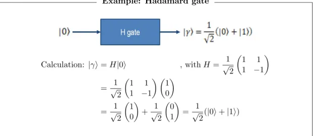
3.3 Example of a gate operation: the Hadamard gate. . . 18

3.4 Example of a gate implementation of Step II of Shor’s algorithm. . . 19

3.5 Building blocks of modular exponentiation, derived from [1].. . . 20

3.6 Method for determining the required resources for running Shor’s algorithm. 22 4.1 Abstract representation of the error-correction steps. . . 26

4.2 Fowler’s choices to select the relevant quantum circuits. . . 29

4.3 Scope and design choice made for estimating the required logical resources for the modular exponentiation circuit. . . 30

4.4 Steps to estimate the amount of physical qubits needed to produce the required ancilla states and parameters influencing this number. . . 31

4.5 A visualization of ion-trap qubits with two different spin directions.. . . . 34

4.6 A basic equivalent circuit for superconducting qubits. . . 36

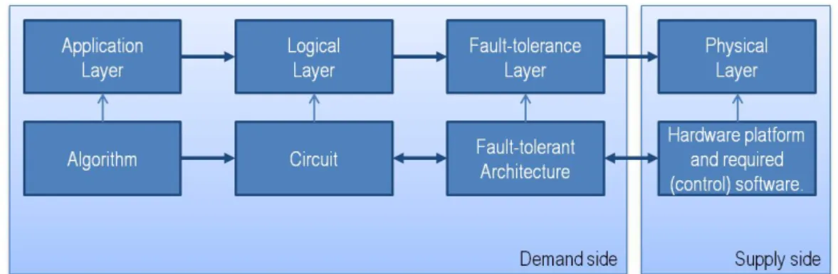
4.7 Layers grouped in a demand side and a supply side in relation to the physical resources. . . 37

5.1 Visualization of the options and choices made. . . 40

5.2 Visualization of the framework for monitoring the quantum threat. . . 53

D.1 Types of Quantum Computing. . . 68

1.1 Overview of research questions and chapters. . . 6

2.1 Impact of Quantum Computing on Common Cryptographic Algorithms. . 12

3.1 Overview of proposed circuit design’s for Shor’s algorithm.. . . 23

4.1 Requirements for implementing a surface-code architecture. . . 28

4.2 Estimates for the required logical building blocks of Shor’s algorithm. . . 31

4.3 Estimates of the required amount of physical qubits for Shor’s algorithm. 32

4.4 A time estimation for Shor’s algorithm using the Fowler et.al. set-up. . . 32

4.5 Estimates of the requirements for implementing Shor’s algorithm using a surface-code architecture on a physical platform. . . 33

C.1 Eigenstates of the two-qubit operatorsXaXbandZaZband the four

eigen-states for this example of non-destructive error-detection. . . 65

Chapter 1

Introduction

1.1

Context

The idea of building a quantum computer already exists for 35 years [2]. Recently com-panies like IBM1 _{and Rigetti}2 _{made quantum computing on real quantum computers}

available in the cloud. Many organizations look with great eager to this new type of computers, because these are supposed to be of great value for research in the field of medicine, material science and energy [3]. Quantum computers also promise to solve computational problems in the research area’s of transport, logistics and artificial intel-ligence [4]. However the opportunities promised by the quantum computer also come at a price.

Several sources, e.g. NIST [5], ETSI [6] and the Dutch NCSC [7] report that the quantum computer is a threat to cyber security. To be more precise: some quantum algorithms pose a threat to some algorithms we use to protect our data. The quantum algorithm proposed by P. Shor poses a threat to cryptographic algorithms based on the (abelian) hidden subgroup problem, such as the mathematical problem of prime factoring as used in RSA [8]. Shor’s algorithm is supposed to solve the factoring problem exponentially faster than known classical algorithms. This would result in breaking RSA, a widely used asymmetric cryptographic algorithm used for key agreement and transport but also for digital signature generation and verification [9].

Another quantum algorithm that poses a threat is Grover’s algorithm. This quantum search algorithm speeds up brute-force attacks on symmetrical key algorithms, such as

1_{IBM Q Quantum experience (https://quantumexperience.ng.bluemix.net/qx/experience, consulted} on 24-10-2017).

2_{Rigetti Forest 1.0 (https://medium.com/rigetti/introducing-forest-f2c806537c6d, consulted on} 24-10-2017) The platform provides a quantum simulator and a quantum chip.

AES. This quantum algorithm also affects secure hash functions, such as SHA-2 and SHA-3. However the speed up Grovers algorithm promises, which is quadratic is, is less compared to the speed up of Shor’s algorithm, which is exponential. Therefore the threat posed by Grover’s algorithm is considered to be less significant [8]. The focus of this thesis is therefore on Shor’s algorithm.

The in this thesis investigated risk event is the event that Shor’s algorithm can be run on an available quantum computer and will break RSA with a 2048 bit key (RSA-2048).

Getting insight in the impact and the probability of an identified risk event is part of the risk analysis phase of a risk assessment. The impact of the defined risk event depends strongly on the context, consequences and current repressive countermeasures. All of these are specific to the organization involved and the responsibility of the person performing the risk assessment, the cyber security specialist.

The probability or likelihood that there is a quantum computer that is able to run Shors algorithm and break RSA-2048, is a general ”feature” from the cyber security specialists point of view. Investigating the likelihood of the risk event is the focus of this thesis.

Some work has been done on this topic, including calculating the cost of running Grover’s algorithm for SHA-256 and SHA3-256 [8]. Also a cost estimation for running Shor’s algorithm to break a 2000-bit number has been reported [10]. These cost estimations can be understood as requirements for a quantum computer and are one of the elements influencing the likelihood of the identified risk event. Another part of the likelihood is assessing if these requirements can be met and, if not, what it takes to close the gap between the requirements and the available resources.

Currently the views on how to deal with the quantum threat differ. One view is that there is plenty of time left for organizations and the other view is to start now with quantum risk assessments [11].

The second objective of this thesis is to determine how to deal with the quantum threat, based on the findings of understanding the requirements to run Shor’s algorithm and break RSA-2048.

1.2

Research questions

3

Sub question 1: What is a quantum computer and which related research is done re-garding the cyber security threat quantum computers pose?

Sub question 2: What is Shor’s algorithm and what are the building blocks on the logical layer?

Sub question 3: How can these logical building blocks be implemented on a practical quantum computer and what are the costs for running Shor’s algorithm for a significant key size?

Sub question 4: What is the gap between the physical resources of current quantum computers and the cost requirements of running Shor’s algorithm for a significant key size?

Sub question 5: Which implementation factors reduce the gap?

The second objective of this thesis is to answer the question: How to deal with the identified quantum threat?

1.3

Methodology

1.3.1 Methodology for answering the research questions related to quantum computing and technology

The quantum computing and quantum technology related research in this thesis follows a methodology derived from methods applied in [8, 10, 12]. Additionally the most likely types of physical implementations and their physical resources are compared to the cost required to run Shor’s algorithm to determine the gap between the supply side, represented by the physical layer and the demand side, represented by three layers. These three layers are the application layer, the logical layer and the fault-tolerant layer. The used method is shown in Figure1.1.

Figure 1.1: Method to determine the requirements for running Shor’s algorithm and

the gap between the demand side and the supply side.

Two experts from different quantum research niches reviewed the assumptions made in this thesis. These experts are R. Versluis and C. Schaffner. Dr. Christian Schaffner3

is professor at the institute for logic, language and computation (ILLC) at University of Amsterdam and works as a researcher at QuSoft. Ir.Richard Versluis4 is a principal scientist/systems engineer at TNO and lead scientist for TNO at QuTech.

In this research only public sources are used as information source. The focus is on literature written by researchers in the quantum domain and the predictions made by quantum experts.

To obtain sufficient knowledge about Shor’s algorithm, information is used from lecture notes and other public sources used to teach university students Quantum Computing or Quantum Information Processing. As with all algorithms, Shor’s algorithm needs to be made ”mechanically” in order to run it on a computer. For this circuits are used. This defines the next step, to look at different logical implementations of Shor’s algorithm using logical quantum circuits. Most information on this topic is obtained from review papers summarizing differences between quantum circuits implementing Shor’s algorithm.

To answer the third research question a literature study is performed to investigate the practical building blocks and requirements needed to run the quantum circuit. We have chosen to focus on the most mature technologies, these are obtained from recent scientific review papers. The fourth research question is answered after a short inventory of the main physical implementations. To answer the fifth research question the most costly building blocks on the demand side are selected and on the supply side a selection is based on the requirements from the demand side.

3_{https://www.cwi.nl/people/2134} 4

5

1.3.2 Methodology for answering the research question how to deal with the quantum threat

To answer the last research question, first a reflection on the likelihood of the risks related to the quantum threat was given based on the findings from the previous research questions.

Also a reflection on the impact of the quantum threat was given. Additional to what was found in the literature on the technical impact of the quantum threat an observation was made that the crypto-systems that are vulnerable to the quantum threat are frequently applied as risk controls to mitigate a risk to an acceptable risk level. This observation is used to develop a method for translating the technical impact of the quantum threat to the impact on the strategic risks of an organization.

The information published by ETSI is used to formulate the impact of the quantum threat on society. A description of the actors involved in the response to the quantum threat regarding cyber security is given based on information from the Dutch second national cyber security strategy (NCSS 2).

The reflections on impact and likelihood are used to reflect on an existing quantum risk assessment methodology by Mosca & Mulholland and two other options, delaying an action plan and mitigation without risk-assessment. A new method for handling the quantum threat is proposed using the findings from the reflection on likelihood and impact.

The proposed monitoring framework uses the findings from research question 5 and the information from standardization institutes ETSI and NIST to determine the topics to monitor. Information from the NCCS2 is used the determine the actors involved for providing the obtained information from monitoring to the relevant parties.

1.3.3 Limitations of the research and intended audience

The literature review to investigate the resources required to run Shor’s algorithm and break RSA-2048 was limited to public sources. A selection from the large amount of available and suitable material, has been made consulting experts.

Another limitation was to use RSA-2048 to determine the physical requirements. There are other crypto-systems vulnerable for the quantum threat, which will lead to other physical requirements and other gaps. To make a more complete analysis of the quantum threat, these other algorithms and their physical requirement should be investigated.

This thesis has been written for people working in the cyber security field with a back-ground in risk management and who are familiar with risk-management standards like NEN-ISO/IEC 31010. Only a general background in quantum mechanics, computer science, information science or electronics is needed to read the complete thesis. Some basic math is required from the reader as well as knowledge about RSA. Readers with no background in quantum mechanics, computer science, information science or electronics can skip Chapters3and 4to get an overview of the results and the reflection on how to deal with the quantum threat.

The thesis uses a high abstraction level, more details on topics can be found in the relevant literature used in each chapter. A more detailed mathematical and physical description of quantum mechanics can be found for example in [2,13].

1.4

Thesis structure

The research questions are answered using the following thesis structure.

Sub question Chapter answering the

sub question

1: What is a quantum computer and which related research is done regarding the cyber security threat

quantum computers pose?

Setting the scene

2: What is Shor’s algorithm and what are the building blocks on the logical layer?

Shor’s algorithm and logical building blocks for implementation

3: How can these logical building blocks be implemented on a practical quantum computer and what are the costs of running Shor’s algorithm for a significant key size?

Fault-tolerant implementations and hardware options 4: What is the gap between the physical resources of current

quantum computers and the cost requirements of running Shor’s algorithm for a significant key size?

Fault-tolerant implementations and hardware options 5.Which implementation factors reduce the gap? Fault-tolerant

implementations and hardware options How to deal with the identified quantum threat? Reflection on

the quantum threat Conclusions and recommendations for further research Conclusions and further

research

Chapter 2

Setting the scene

Most cyber security experts are familiar with threats in the classical domain1. For exam-ple, vulnerabilities in IT systems or industrial control systems, vulnerabilities resulting from the human component in IT, such as attackers using social engineering to get ac-cess to information or IT systems and vulnerabilities resulting from procedures, such as inadequate patch management.

To understand the cyber security threat a quantum computer poses, a brief introduction in the quantum field is necessary. This chapter starts with a brief introduction about what a quantum computer is and closes with more background information on the threat quantum computers pose to cyber security. The threat quantum computers pose is often referred to as the quantum threat. In this thesis both are used.

2.1

What is a quantum computer?

The definition of a quantum computer strongly depends on the scientific field and the background of the audience. For the purpose of this thesis a general definition is chosen:

A quantum computer is a computing device that exploits quantum-mechanical phenom-ena, such as superposition, entanglement and interference.

This definition is derived from a similar definition as published in [14]. The next two sections provide more information on the quantum mechanical phenomena and the com-puting device.

1_{People working in the in the scientific fields related to quantum mechanics, quantum computing,} quantum information theory etc, use the term classical for the world as we know it or everything that is not using the unique quantum mechanical features explicitly. Note that the term conventional is also used.

2.1.1 Quantum-mechanical phenomena

The computational power of a quantum computer is based on three phenomena: quan-tum parallelism, entanglement and quanquan-tum interference. These phenomena provide quantum algorithms the computational power to solve certain mathematical problems more efficiently than classical computers solve these problems.

Quantum parallelism uses the quantum feature of superposition to apply a function2 to all possible input values simultaneously. Superposition allows quantum systems to be in many different states at the same time [13]. Quantum systems are used to store infor-mation. The most simple quantum system is a qubit. In press releases, superposition is often translated as: a qubit can be 1 and 0 at the same time.

”Entanglement arises when two or more quantum systems exist in a superposition of correlated states.”[15]. If for example two qubits were entangled and separated physical from each other3, then the operations performed on the first qubit would affect the second qubit instantaneously independent of the distance between them. These are called non-local effects and refer to what Einstein called ”spooky action at a distance” [13].

The effects of interference on an algorithm can be best compared with interference pat-terns between light or sound waves [13]. Depending on the applied interference, some quantum states cancel out and some are amplified. When measuring a quantum state to obtain the output of an algorithm, this amplification means that the probability of ob-taining a measurement result (output) from that amplified quantum state increases and the probability of obtaining a measurement state from a less amplified state decreases.

2.1.2 Computing device

Here we formulate a computing device as a system with an input, some computation (evolution) and an output, see Figure 2.1. For example: Shor’s algorithm has as input, integer N = pq, where p and q are large prime numbers. The goal is to compute the prime factors p and q as desired4 output. Quantum computation can be defined as ”a sequence of unitary transformations, affecting simultaneously each element of the superposition, generating a massive parallel data processing albeit within one piece of quantum hardware” [16].

2

Algorithms apply one of more mathematical function(s).

3_{For example: one qubit stays in The Hague (city in Europe) and the other is transported to a city} in Australia.

9

Figure 2.1: Computing device using an input to produce an output.

A quantum computer needs a quantum state as input. The most simple quantum state is a qubit. The state of a qubit can be visualized as a point on a unit three-dimensional sphere,the Bloch sphere, as visualized in Figure2.2.

Figure 2.2: Bloch sphere representation including three different qubit states |0i,

|1i, |ψi=α|0i+β|1i, where αandβ are complex numbers. Because|α|2_+|β|2 _{= 1,}

|ψi=α|0i+β|1i=eiγ cos₂θ|0i+eiφsinθ₂|1i

, whereθ,φandγare real numbers. Since

eiγ_{has no observable effects, this term is omitted, resulting in|ψi=cos}θ

2|0i+e

iφ_sinθ

2|1i [2].

After initialization of the quantum state (the input), the quantum state is evolved to an output state using a quantum circuit with quantum gates. During the execution of the algorithm the quantum states may suffer from an effect called decoherence.

Decoherence is a kind of noise that has no classical analog. A simplified model of deco-herence is described by two parameters acting in parallel, phase damping and amplitude damping. Phase damping describes the loss of quantum information without loss of energy [2]. It is called phase damping, because it randomly changes the phase of a quan-tum system reducing the coherence between the superposed |0i and |1i states and by this leaking information. Phase randomization has timescale T2 [2,17]. Phase damping

is visualized in Figure 2.3. Phase damping affects the xy-plane of the Bloch sphere,

x1 6=x2 and y1 6=y2.

Amplitude damping refers to the effects due to energy loss in a quantum system [2]. For example if a qubit in superposition, |ψi=α|0i+β|1i, where |α|2_+|β|2 _{= 1, loses}

Figure 2.3: Visualization of phase damping. On the left the Bloch sphere without phase damping effects, thexy-plane forms a perfect unit circle. On the right the Bloch sphere with phase damping effects, thexy-plane is not forming a perfect unit circle.

driving the qubit to its ground state. Amplitude damping, or relaxation, has timescale

T1. In principle the physical qubit relaxation timeT1 and the physical de-phasing time

T2 determine the coherence time.

When an algorithm is executed errors occur, due to decoherence and other effects like control errors and measurement errors. To execute an algorithm successfully all required computational steps should be completed with a low error rate per computational step. The error rate limits the practical number of computational steps that can be executed by a quantum computer. However by encoding quantum information in multiple physical qubits, the available execution time can be increased to exceed significantly the physical coherence time of the physical qubits. To encode quantum information in multiple physical qubit states quantum error correction (QEC) codes are used.

Example: Quantum Error Correction Code

Quantum systems can protect a single quantum state, e.g. |1i, by encoding this quantum state using three quantum states, creating redundancy in the information. The resulting protected quantum system is called a logical quantum state and is stored in three qubits.

|1>→ |1i_L≡ |111i, where Lstands for logical state.

The logical quantum state|1i_L representing a bit of information with value one is encoded in three physical qubits|111i.

11

There are many QEC codes and they all have their own properties. QEC codes use the notation [n, k, d], where n represents the number of physical qubits, k denotes the number of logical qubits, andd is the distance of the code [18]. The number of errors5 a code can correct depends on the code distance d.

Using QECs to protect the information stored in the quantum system as it dynamically undergoes computation is called fault-tolerant quantum computation [2]. By increasing the code distanced, arbitrary low logical error rates can be achieved. In an architecture realizing fault-tolerance different QEC codes can be used to achieve arbitrarily good quantum computation. Which QEC codes are optimal and which corresponding values of d, depend on the the type of error model, the quality of the physical qubits and architectural considerations, such as the connectivity between qubits. A fault-tolerant architecture can be realized [19]. It will however come at a price, which is reflected in the requirements on the physical resources, see Chapter4 for more details.

In the end, when the input quantum state has been evolved to the final quantum state, a measurement needs to be done to obtain the results from the computations. The effects of superposition, a quantum state being in multiple states at the same time, ends when measuring this state. During measurement, using a computational basis (|0i and |1i), the quantum state is forced into one of many quantum states. For example, a qubit in superposition (|ψi =α|0i+β|1i) is forced into a 1 or a 0, it cannot be both. The probability6 of measuring the desired output should be high to increase the success rate of running the algorithm.

Figure 2.4: General visualization of layers needed for the physical realization of a

quantum computer, derived from [20].

To realize a computing device with a fault-tolerant architecture and the capability to initialize quantum states, to perform computational steps and to measure the final quan-tum states, physical building blocks are required. A physical realization of the quanquan-tum computer consists not only of a quantum chip, but also includes the complementary hardware and software. This is represented by the bottom three layers of Figure 2.4.

5

”The distance between two code words states,d, defines the number of errors that can be corrected,

t, as,t=b(d−1)/2c”[19]. 6

Measuring results in either 0 with probability|α|2

The bottom layer, the quantum chip, holds the physical qubits which are structured to enable a fault-tolerant architecture. These physical qubits need to be controlled, to enable physical qubit operations including measurements for error detection, this is represented in the control electronics layer. The compiler layer enables optimization, error corrections and logical operations [20]. Chapter 4 will provide information about two types of physical qubit implementations, also referred to as qubit technologies and quantum chips.

2.2

The quantum threat and cyber security

In 2016 NIST published a table summarizing the threat quantum computers pose, see Table 2.1. NIST explains that many communication protocols use three core cryp-tographic functionalities: public-key encryption, digital signatures, and key exchange. Diffie-Hellman key exchange, the RSA cryptosystem, and elliptic-curve cryptosystems are mostly implemented to fulfill these functionalities [5]. However their security depends on the difficulty of solving problems such as integer factorization or the discrete-log prob-lem over various groups.

In [21] P. Shor showed that both problems can be efficiently solved on a quantum com-puter, and -as the NIST publication puts it- ”thereby rendering all public-key cryp-tosystems based on such assumptions impotent” [5]. The quadratic speed up of Grover’s search algorithm has a less significant impact. The NIST publication explains that cryp-tographic systems should not be considered obsolete, but there will be a need for larger key sizes even for symmetric-key algorithms [5].

Cryptographic Algorithm

Type Purpose Impact from

large-scale quantum com-puter

AES Symmetric key Encryption Larger key sizes needed SHA-2, SHA-3 ————— Hash functions Larger output needed

RSA Public key Signatures,

key establishment

No longer secure

ECDSA, ECDH

(Elliptic Curve Cryptography)

Public key Signatures, key exchange

No longer secure

DSA (Finite Field Cryptography)

Public key Signatures, key exchange

No longer secure

Table 2.1: Derived from NIST Table - Impact of Quantum Computing on Common

13

Similar work is provided by other institutes, like ETSI. They provide a comparison of security levels, both conventional and quantum, for some popular ciphers including RSA, ECC and AES [6].

The NIST publication states that only a ”large-scale quantum computer” will impact the discussed cryptographic algorithms [5]. About the likelihood that there is or will be a large scale quantum computer, the NIST publication only refers to predictions from experts. ”While in the past it was less clear that large quantum computers are a physical possibility, many scientists now believe it to be merely a significant engineering challenge. Some experts even predict that within the next 20 or so years, sufficiently large quantum computers will be built to break essentially all public-key schemes currently in use” [5]. For this prediction NIST used the estimates made by expert M. Mosca. Section 2.2.1

will elaborate more on his work.

2.2.1 Related work

M. Mosca derived a simple model to determine when it is time to prepare for the quantum threat, Mosca’s ”x, y, z” quantum risk model. This model includes the duration that information should be kept secure (x), the time it takes to migrate to a quantum-safe solution (y) and an estimate on when identified threat actors have access to quantum technology (z) [22], see also Section5.3.2.

To determine z, when threat actors get access to a large-scale quantum computer, M. Mosca makes estimations”one in seven chance that some of the fundamental public-key cryptography tools upon which we rely today will be broken by 2026 and a 50% chance by 2031.” [23, 24]. These estimates are based on several key values, in Mosca’s paper three of these values are described [24].

The first value is: ”When will we reach the design of a fault-tolerant scalable qubit?” A target date of the year 2021 was given in 2015 by an IARPA7announcement for proposals to build: ”a logical qubit from a number of imperfect physical qubits by combining high-fidelity multi-qubit operations with extensible integration” [24]8.

The second value is: ”How many physical qubits will we need to break RSA-2048? . . . Current estimates range from tens of millions to a billion physical qubits.” These estimates depend on a lot of factors. Mosca names a subset: the efficiency of fault-tolerant error-correcting codes, the physical error models and error rates of the physical quantum computers, optimizations in the quantum factoring algorithms, and the effi-ciency of the synthesis of factoring algorithms into fault-tolerant gates [24].

7

Intelligence Advanced Research Projects Activity (IARPA) US Government. 8

The last value is: ”How long will it take to scale the scalable design to the size sufficient to break RSA-2048?” Mosca notes that the rate of scaling depends on the availability of tools, some of which are already available and some of which are being developed [24]. For the second value given by Mosca, a kind of structured approach is provided in Appendix M of a paper by Fowler et. al. [10]. In this appendix they estimate the amount of physical qubits for running Shor’s algorithm to factor N = pq, with N of size 2000 bits, based on a surface-code implementation for fault-tolerance. Similar work is done by Amy et. al. for running Grover’s algorithm to break SHA-256 and SHA3-256 in [8]. Both use a similar method: choose the algorithm you wish to run, choose a circuit implementing the algorithm (or design/optimize a circuit), choose a fault-tolerant implementation and determine the required number of physical qubits and other physical resources.

These physical resources need to be available on a quantum computer in order to run the algorithm using the circuit. There are many different options for implementing the required physical building blocks. Two papers, one using spin qubits and the other using Josephson charge qubits, have implemented Shor’s algorithm factoring, integersN = 15 and N = 21 [25,26]. These papers omit the fault-tolerant implementation and directly implement the circuit on the physical layer. They do however provide a bridge between two separate research fields, the research field studying quantum algorithm and the field studying the physical realization of quantum building blocks [26].

Not only the realization of the physical building blocks is important but also the way these building blocks work together. In a paper by R. van Meter et al. is stated that the architecture used for the realization of a quantum computer ”can make the differ-ence between an interesting proof of concept device and an immediate threat to all RSA encryption”[27]. He makes this concrete by comparing the best known classical threat to RSA, the number field sieve, with Shor’s algorithm implemented on different archi-tectures running with different clock speeds. For a N of size 1000 bits the best known classical algorithm takes more than a thousand years to factor N. The time needed to factor a N of this size using Shor’s algorithm on different architectures ranges from seconds to more than a thousand years [1].

Chapter 3

Shor’s algorithm and logical

building blocks for

implementation

This chapter investigates the building blocks needed to run Shor’s algorithm efficiently. First a description of Shor’s algorithm is given, followed by an introduction on quantum circuits. These quantum circuits are used to implement algorithms. An overview is provided of quantum circuits relevant for Shor’s algorithm and this chapter closes with a reflection on the general building blocks needed to run Shor’s algorithm for a 2048-bit integerN =pq.

3.1

Shor’s Algorithm

In 1994 Peter Shor showed that two important problems, for which we do not know any efficient classical solution, could be solved efficiently on a quantum computer. He gave a quantum solution for the problem of finding the prime factors of an integer and a solution for the so-called discrete-logarithm problem [21].

In his paper, P. Shor shows that the problem could be solved in polynomial time by dividing it in four steps [21]. To achieve this speed up only one of these steps, Step II, needs to be executed on a quantum computer. The other three steps are executed on a classical computer [15].

Shor’s Algorithm

LetN =pq for two large prime factorspand q. In order to findp andq, follow the steps below.

• STEP I: Choose x such that 1< x≤N −1.

Compute the Greatest Common Divisor (GCD) ofx andN to make sure that they are relative prime (GCD(x, N) = 1).

Note that if GCD(x, N)6= 1, then GCD(x, N) =p or q and we can stop the algorithm.

• STEP II: Solve the discrete-logarithm problem for a given x and N, i.e. find the smallest hidden period r, such thatxr≡1 mod N.

• STEP III: Check if r is even. Ifr is odd, then restart at STEP I. Ifr is even, then derive:

xr≡1 mod N xr−1 = 0 mod N

xr−1 =cN (where c is an integer.) (xr/2−1)(xr/2+ 1) =cpq

• STEP IV: Calculate p=GCD((xr/2−1), N) and q=GCD((xr/2+ 1), N).

Note for STEP I that the GCD can be calculated using Euclid’s algorithm:

GCD(x, N) :r1 =N mod x, where 0≤r1 ≤x−1 ;r2=x mod r1, where 0≤r2 ≤r1;

r3 =r1 mod r2, where 0≤r2≤r1;. . .;rn= 1;gcd=rn−1 [15].

Note for STEP II the periodicity results from repeated multiplication with x. The sequence: 1 = x1 modN, x2 mod N, x3 mod N, . . ., will start to cycle after a while: there is at least an 0< r≤N−1, for which holdsxr = 1 modN, wherer is called the period of the sequence [13]. For an example, see AppendixA.

Note for STEP III it can be proven that r is even with a probability ≥ 0.5 that and (xr/2−1) and (xr/2+ 1) are no multiples of N. The proof, using basic number theory, can be found in [13] on page 29.

17

3.2

A brief introduction to quantum circuits

To understand how STEP II can be implemented on a quantum computer, the next step on the road to implementation should be investigated: quantum circuits.

Quantum circuits are made of wires and gates that together implement an algorithm. An algorithm is a precise recipe for performing a computational task, e.g. prime fac-torization [2]. A gate maps an input quantum state to an output quantum state. The wires represent the quantum states and show the connections between input and output of the gates. This is summarized in Figure 3.1.

Figure 3.1: The different elements of implementing a computational task.

Figure 3.2 shows an example of a simple quantum circuit. Any quantum operation (gate) can be represented by anM×M complex-valued matrix U, which is an unitary matrix, meaning that its inverse U−1 equals its conjugate transpose U∗. Any quantum operation is by definition reversible.

Example: Simple quantum circuit

Figure 3.2: Example of a simple quantum circuit.

A quantum state (the state of the wire) |φi is represented as a M-dimensional vector (µ1, . . . , µM)T. If a unitary operator transforms this quantum state to an output state |ψi, which is represented by a M-dimensional vector (λ1, . . . , λM)T, then this will be

denoted as |ψi=U|φi or:

       λ1 λ2 .. . λn        =U        µ1 µ2 .. . µn        .

Depending on the complexity of the quantum operation the quantum gate may be built from other gates implementing parts of the quantum operator. There are many different gates. A set of gates is called universal if all other unitary transformations can be built1 from that set [13], see Figure 3.1. Figure 3.3 shows an example of an important single-qubit gate, the Hadamard gate, which maps the input state|0ito an output state

1

√

2(|0i+|1i), a superposition.

Example: Hadamard gate

Calculation: |γi=H|0i , withH = √1

2

1 1

1 −1

= √1

2

1 1

1 −1 1 0

= √1

2

1 0

+√1

2

0 1

= √1

2(|0i+|1i)

Figure 3.3: Example of a gate operation: the input |0i is multiplied by the Hadamard transform implemented by a Hadamard gate. This produces an output

in superposition: _√1

2(|0i+|1i).

A different type of quantum operator is the measurement operator, which is non-reversible. When measuring in the computational basis, the quantum state |φi = (µ1, . . . , µM)T, is forced into the classical state |ji with probability |µj|2, this is the

squared norm2 of the amplitude µj [13]. There are other types of measurements that do

not force a quantum state into a classical state, this type of measurement is needed for a fault-tolerant implementation of Shor’s algorithm and will be addressed in Chapter4. 1_{The set of all single-qubit operations together with the two-qubit CNOT gate is universal [13]. Other} sets approximate any other unitary arbitrarily well using circuits of only these gates. It has been proven in the Solovay-Kitaev theorem that this approximation can be done efficiently [13].

2

Amplitudeµjis a complex numberµj=a+ib, whereaandb∈ Randi2=−1, the squared norm:

|µj|2=

19

In this short introduction to quantum circuits we have seen that algorithms are repre-sented by quantum circuits. These circuits are built using quantum gates and wires. Quantum gates implement unitary transforms which makes the gates reversible. In the next section, Step II of Shor’s algorithm is discussed and visualized using a general circuit implementation.

3.3

The quantum step in Shor’s algorithm

STEP II, finding the smallest period r of x mod N, is called order finding, because in the discrete-logarithm form factoring has a periodic structure [15]. The process of finding the order r can be summarized in six main steps [15,21,25,26].

1. Initialize quantum registers.

2. Generate a superposition on the qubits in the first register.

3. Compute the modular exponentiation: f(x) =ax mod N, for a given N,aand x

and use the second register to store the values off(x).

4. Apply the Quantum Fourier Transform (QFT) to the first register.

5. Measure the first register to get an indication of the period r.

6. Use a classical computer to perform post-processing to obtain the period r.

Figure 3.4 shows a general implementation of Step II, the steps are executed from the left to the right. The lines represent the wires and the blue boxes the gates implementing the quantum operations. The last box on the right (CP) is a classical post-processing step, and not a quantum gate. The steps are briefly explained using various sources [15, 21, 25, 26]. The description of the modular exponentiation, Step 3, also uses the V.Meter’s thesis [1] as a source.

Figure 3.4: Example of a gate implementation of Step II of Shor’s algorithm, derived

3.3.1 Initialization

To start the procedure of finding primes p and q, two quantum registers are prepared. The first quantum register containsn= 2dlog2Nequbits in state|0i, whereN =pq. The

second quantum register contains m =dlog2Ne qubits in state |1i. The first quantum

register is used to store the values of x, the second quantum register will be used to store the values of f(x) =ax mod N.

3.3.2 Superposition

The next step, Item 2 of Figure 3.4, puts the quantum states of the first register in superposition by applying the Hadamard gate to each qubit individually (H⊗n). This results in the state: √1

2n

P2n−1

x=0 |xi|0i. Note this is similar to the example in Section3.2,

only now fornqubits.

3.3.3 Modular Exponentiation and entanglement

Item3of Figure3.4contains two steps, modular exponentiation and entanglement. The modular exponentiation problem is: Compute f(x) =ax _{mod N, for a givenN,a and}

x. The result, the values of f(x), are stored in the second register. Computing the modular-exponentiation problem is considered the most resource-intensive step of the quantum part of Shor’s algorithm, as it consumes the most time and space.

Modular exponentiation is realized using modular multiplication building blocks, which on their turn are realized using blocks that perform modular addition. These last blocks are built from blocks performing addition and comparison, see Figure3.5. The construc-tion of the modular multiplicaconstruc-tion using these two building blocks can be compared to a classical variant of writing an exponent as a set of multiplications and a multiplication as a sum. Mathematically: αβ =α·α· · · · ·α

| {z } β times

and ν·µ=ν+ν+· · ·+ν

| {z } µ times

.

Figure 3.5: Building blocks of modular exponentiation, derived from [1].

21

Entanglement

The next step is to use a unitary operator Uf to entangle the input state x with the

corresponding value of f(x), this results in the state: √1

2n

P2n−1

x=0 |xi|ax modNi. This

state is periodic with (hidden) period r.

The periodicity results from repeated multiplication with x. The sequence: 1 = x1

mod N, x2 mod N, x3 mod N, . . ., will start to cycle after a while: there is at least an 0 < r ≤ N −1, for which holds xr = 1 modN, where r is called the period of the sequence [13]. For an example, see AppendixA.

3.3.4 Quantum Fourier Transform

Using the Quantum Fourier Transform as a quantum operator, realizes the quantum-mechanical phenomena of interference. Applying the inverse Quantum Fourier Trans-form (QF T−1) to the first register reveals the periodic property of the created state. This results in: ₂1n

P2n−1

x,y=0exp (2πixy/2n)|yi|ax mod Ni. Positive interference, the

am-plification of the amplitudes, occurs wheny=c2_rn, for an integerc. For more detail see AppendixB.

3.3.5 Measurement

In this step the first register is measured. The positive interference caused a high prob-ability of obtaining measurement resulty for which holds that ₂yn = _rc, where y and 2n

are known and c and r not. Note that the exact value3 of this probability depends on the value of r, the integer c and n, more information can be found in Shor’s extended paper [21].

3.3.6 Classical post-processing

The last step, Item 6 of Figure 3.4, is to extract period r out of the obtained ₂yn = _rc.

To find this period a technique called Continued Fraction Approximation is used. This technique can be implemented and run efficiently on a conventional computer, using classical computation. The mathematical steps can be found in e.g. [13].

These six steps are part of STEP II of Shor’s algorithm, the process of finding the orderr. We have seen that Shor proposed an probabilistic algorithm which factorsN =pq, with large primespandq, in four steps I-IV. The proposed algorithm does not only utilize the quantum-mechanical phenomena like superposition, entanglement and interference but also needs classical computation, that can be run efficiently on a conventional computer.

3

The probability of obtaining the required output will be at least ₃1_r2 if|{rc}2n| ≤ r

3.4

Quantum circuits relevant for Shor’s algorithm

To investigate the likelihood that there is a quantum computer that can run Shor’s algorithm efficiently we focus on the most resource-intensive step of the quantum part of Shor’s algorithm, the modular exponentiation. This part of the algorithm will dominate the physical requirements that are needed on a quantum computer [21].

To understand the physical requirements, first the logical requirements need to be inves-tigated. Figure3.6shows the different layers for analyzing Shor’s algorithm. The logical requirements depend on the optimization choices or restrictions applied while designing a modular exponentiation circuit. Providing insight in these design choices is the topic of the next section.

Figure 3.6: Different layers and the elements of these layers for analyzing the different

resources required for running Shor’s algorithm, based on [8].

3.4.1 Comparing quantum circuits

The quantum circuits discussed in this chapter, are executed in the logical layer, see Figure 3.6. These quantum circuits are compared using two parameters: The first parameter is the number of required logical computational qubits (wires) also referred to as thecircuit width. The circuit width gives an indication for the space the quantum circuit requires. The second parameter is the logical circuit depth.

The circuit depth is defined as the number of sequential gates within a circuit [28]. This parameter is used as an indication for the duration of the algorithm. The actual execution time will depend on the implementation on the physical layer and on the different physical gate and measurement times4. However, to allow an early comparison of different circuits, the duration of all gates and measurements are assumed the same. This enables to express the duration or circuit depth in the number of gates.

23

representation. Note the big O notation is also used for the comparison or analysis of algorithms in the field of classical computer science.

3.4.2 Overview of quantum circuits relevant for Shor’s algorithm

In 2005 S. Devitt, A. Fowler and L. Hollenberg published an overview [28] of proposed circuit designs for modular exponentiation (Item3in Figure3.4), their results are sum-marized in Table3.1. The results provided are accurate to the leading order inm, where

m=log2(N) andN is the integer of bit lengthm that needs to be factorized.

Circuit’s optimiza-tion criteria Number of Qubits Circuit Depth Reference

Conceptual simplicity _v5m O(m3_{) ”V.Vedral, A.Barenco, and A.Ekert,} Quantum Networks for Elementary Arithmetic Operations, Phys. Rev. A 54, p. 147, 1996.”

Running time O(m2_{) O(mlogm) ”P. Gossett, Quantum carry save} arith-metic, quant-ph/9808061, 1998.” Number of qubits _v2m

(2m+ 3)

v32m3 ”S. Beauregard, Circuit for Shors al-gorithm using 2n+3 qubits, Quan-tum Information and Computation 3, p. 175, 2003.”

Time/Space - Trade-off I

v50m _v219_m1.2 _{”C.Zalka, Fast versions of Shors} Quantum Factoring algorithm,quant-ph/9806084, 1998.”

Time/Space - Trade-off II

v5m _v3000m2 _{”C.Zalka, Fast versions of Shors} Quantum Factoring algorithm, quant-ph/9806084, 1998.”

Table 3.1: Overview of proposed circuit design’s for Shor’s algorithm.

Each quantum circuit is designed with some design objective or an optimization goal. For example the Beauregard circuit, third row in Table3.1, is designed using the design criteria: Minimize the number of (logical) qubits needed for factorization in polynomial time.

The results above are just a snapshot in time. The field of quantum circuit design is continuously improving. For example in v. Meter’s PhD thesis additional circuits are described. Most of these other circuits focus on reducing circuit depth for the adder gate building block [1]. When the the circuit depth and the number of gates is reduced, the number of computational qubits will increase, this is also referred to as the time/space - trade-off.

In a paper by A. Fowler et.al. [10] modular exponentiation circuits are compared using different parameters. This paper relates more to the fault-tolerant layer of Figure 3.6

and therefore considers the parameters: the number of computational logical qubits, the sequential number of Toffoli gates, and the total number of Toffoli gates. The reason for choosing these parameters is, that the physical size of the circuit scales with the ratio of the total number of Toffoli gates to the number of sequential Toffoli gates. To realize practical large-scale quantum computing, circuit designers should therefore minimize the number of these Toffoli gates used in their circuits.

3.5

Logical building blocks for running Shor’s algorithm

For Shor’s algorithm the building blocks can be roughly summarized as quantum state initialization, unitary transforms, measurement operations and classical processing. On the quantum logical layer the first three building blocks are translated to circuits using logical gates and logical qubits.

The required logical resources depend on design choices or optimization’s applied when designing the circuits. When making these choices there is always a trade-off between the number of logical qubits and the number of logical sequential gates. This also known as the time-space trade-off, as the number of logical sequential gates give an indication for the duration of the computation and the logical qubits indicate an amount of space the circuit occupies.

For example Beauregards circuit minimizes the required logical qubits to implement Shor’s algorithm. This circuit requires approximately 2m logical qubits and 32m3 log-ical sequential gates, where m is the bit length of the integer N = pq. Resulting in approximately 4099 logical qubits and approximately 275·109 sequential logical gates form= 2048 bits.

Chapter 4

Fault-tolerant implementations

and hardware options

As we have seen in the previous chapter, the logical resources are significant for imple-menting the modular exponentiation circuit for a N =pqof 2048 bits. Recall that it is unrealistic to assume that running these large circuits will be without any errors, when these circuits are implemented on physical building blocks. To investigate the require-ments for a quantum computer, which can run Shor’s algorithm efficiently we need to discuss quantum-error-correction (QEC) techniques.

QEC techniques make the realization of large-scale practical quantum computers feasible by extending the possible execution time of a quantum state and by correcting errors that occur. Fault-tolerance architectures use these QEC-techniques. Fault-tolerance architectures are architectures that are designed to keep control over errors and as a result enable large-scale quantum computation. Fault-tolerance architectures are the topic of this chapter.

4.1

Fault-tolerant quantum computing

In a recent review by E. Cambell, B. Terhal and C. Vuillot different roads towards fault-tolerant universal quantum computation are discussed [18]. In this review the surface code is positioned as a promising architecture, because of its high-noise threshold, the requirements of only 2-dimensional (2D) qubit connectivity and a T-gate that is relative cheap to implement regarding the space-time overhead1.

1_{The space overhead or spatial overhead is formulated as the number of physical qubits that are} needed to form a logical qubit. The time overhead or temporal overhead is the difference in gate execution on a physical gate and on a logical gate [18].

A high-noise threshold is convenient, because the noise should always stay below the noise threshold. Fault tolerance can only be achieved if the physical-error rate2 stays below the noise threshold [18,19, 29]. If this is achieved, then arbitrary long quantum computations are possible with arbitrary accuracy[2]. This limits the impact of deco-herence and faulty quantum gates [18] and make it possible to run Shor’s algorithm successfully for a large N, such as 2048-bits. Note that the threshold is not a fixed value, but it depends on multiple variables: the type of error model(s) applied, the QEC method and architectural considerations, e.g. how the qubits can interact [18,19].

4.1.1 Surface code

A fault-tolerant architecture can deal with errors as long as these errors can be identified. Once these errors are identified, errors can be corrected in any subsequent (measurement) operation. For the fault-tolerant architecture named surface code this is done using classical control software, e.g. Edmonds’ minimum-weight perfect-matching algorithm. This algorithm works perfectly for sufficiently sparse errors, but fails when the density of errors increases [10]. Figure4.1gives an abstract representation of the steps taken by the surface-code architecture to perform error correction.

Figure 4.1: Abstract representation of the error-correction steps.

Error detection

In order to ensure that the measurements, which are needed to identify the errors, do not destroy the quantum system, the surface code applies a special type of procedure for measurements. The quantum systems are repeatedly measured using a complete set of commuting3 stabilizers. An example for a two-qubit system is given in AppendixC. Stabilizers are operator products and measure multiple quantum systems simultaneously. Following this procedure the quantum system is forced into a simultaneous and unique eigenstate of all the stabilizers, which preserves (stabilize) the quantum properties of

2_{The physical-errors occur due to information leakage, measurement errors, control errors,} decoher-ence etc.

3

27

the state. The detecting property follows by comparing measurement results. If the measurement outcome is changed compared to earlier measurement results (eigenvalues), then one or more errors are detected. The measurement outcome is the eigenvalue and the measurement projects the quantum state into a stabilizer eigenstate [10].

The errors that are identified are stored in a Pauli frame. The Pauli frame functions as a memory that is updated each code cycle [30]. As with classical errors some quantum errors cancel each other out [10]. This gives the opportunity to optimize the error processing. It depends on the optimization choices that are possible on the hardware platform and the sequence of logic gate operations of the quantum circuit, when the information from the Pauli frame4 is used to correct the errors [29]. Section 4.3 will provide information about the hardware platforms.

Logical operations

The surface code architecture is not complete if it is not able to facilitate logical-gate operations. The logical operations are built from the fault-tolerant Clifford+T-gate set. The Clifford+T-gate set is an important universal gate set [18].The Clifford gates are generated by the Hadamard gate, the S-gate5 and the Controlled NOT (CNOT)-gate. However to achieve an universal gate set and to add quantum-computational advantage a non-Clifford gate should be added6, this is the T-gate. The T-gate is a single qubit

gate, represented by T = 1 0 0 eiπ/4

! .

The properties of the surface-code architecture allow to create a logical qubit state and the logical gate set. There are multiple options to realize these logical Clifford-gates. Some examples, derived from [10], are given below:

• A logical qubit is created e.g. by entangling multiple physical qubits, using physical CNOT operations and subsequent measurements.

• A logical qubit is initialized e.g. in an eigenstate of a qubit cut or hole. Holes are

created by turning off measurement qubits.

• A logical Hadamard operation is created by physical Hadamard gates and SWAP7 operations.

• The logical CNOT is created by e.g. a braid transformation8_{, which can entangle}

two qubits.

4_{Note that after the information from the Pauli frame is used the Pauli frame is emptied to restart} the collection of information.

5_{S=diag(1, e}iπ/2₎ 6

Recall that with a universal gate set all quantum computations can be built. 7

A swap is an exchange of quantum states between qubits [10]. 8

To create a logical T-gate9 multiple techniques are possible, however the most promising solution for this is magic-state distillation [18]. This magic-state distillation is also referred to as state distillation or ancilla state distillation [10].

Magic states are realized via a procedure that filters noisy quantum states to better quality states [18]. For this error-correcting codes and circuits, which involve single-control multi-target logical CNOTs, are used [10]. The T-gate is then realized using the magic states via a simple fault-tolerant circuit. Note that the T-gate is a few hundred times as costly as the Clifford gates in terms of space-time overhead and is therefore the most resource intensive building block [18].

Requirements for implementing a surface code architecture

The combination of state distillation and surface code is considered a competitive scheme and currently this combination is the most practical option to create a fault-tolerant architecture. If this practical most promising architecture is not suitable for requirements and other constrains, then alternatives are possible. However these alternatives are work in progress, e.g. work is needed to improve the noise threshold to be comparable with the noise threshold of surface code [18].

Requirements for physical implementations Values

Minimum physical single-qubit gate fidelity 99% Minimum physical two-qubit gate fidelity 99%

Minimum measurement fidelity 99%

Table 4.1: Requirements for implementing a surface-code architecture.

The requirements given to implement surface code on a physical platform are given in [10]. Table4.1 gives a summary of these requirements.

Section4.3 provides insight if the current specifications of hardware platforms are able to meet these requirements. First another requirement is derived, the number of physical qubits required to run Shor’s algorithm on a surface code architecture.

4.2

A cost estimate for running Shor’s algorithm

From the previous section we have learned that the combination of state distillation and surface code is considered a competitive scheme [18]. Appendix M of the paper on surface code by A. Fowler et.al. [10] gives an estimate of the amount of physical

9

29

qubits for running Shor’s algorithm to factor a 2000-bitN =pq, using this competitive scheme10. This sections provides a summary and a reflection on the steps taken and results derived by Fowler et.al.

4.2.1 Circuit selection

Fowler et.al. starts with selecting a circuit that implements Shor’s algorithm which is followed by a selection of the quantum adder circuit, see Figure 4.2. The selection criteria is to minimize the number of Toffoli gates, which in the end minimizes the required physical resources. More information about what a Toffoli gate is, can be found in AppendixC

Figure 4.2: Fowler’s choices to select the relevant quantum circuits.

4.2.2 Determine the required logic resources

The next step is to determine the number of required basic logic resources for the most resource-intensive part of the circuit. The logical resources are derived using the number of logic Toffoli gates the circuit requires for factoring a 2000-bitN =pq. Toffoli gates are build from T-gates, which need highly distilled ancilla states. The ”factories” producing these ancilla states consume the most physical resources [10]. Figure4.3shows the steps Fowler et.al. take to estimate the number of logic ancilla states.

Figure 4.3: Scope and design choice made for estimating the required logical resources

for the modular exponentiation circuit.

4.2.3 Determine the required physical resources

The ancilla states needed for the T-gate should meet two requirements to ensure that the modular exponentiation circuit makes negligible errors, which is needed for a proper functioning of Shor’s algorithm. The first requirement is that the ancilla states are produced at a sufficient rate to keep pace to the modular exponentiation circuit. The second requirement is that the produced ancilla states should have a sufficiently small logical error rate. To ensure a good fidelity of the circuit the final logic error rate of

|ALi should be of the order 10−14−10−15.

This final logic error rate is achieved by multiple distillation stages. In the set up proposed in the paper by Fowler et.al. each distillation stage improves the error rate by

pnew =cp3input, where c is a characteristic of the distillation circuit with value c= 35.

Fowler et.al. assumes apinput = 0,005 as the initial error rate as input for the distillation

process.

The distillation circuit is implemented in surface-code to compensate for the errors, assuming an error probability per surface code cycle of p = 0,01, which results in a required fidelity of 99,9%. To minimize the total footprint11 of the required circuit, the surface-code distance of the first stage is reduced. This is possible because the following stage will distill the remaining errors in order to achieve the required logic error rate.

Each distillation stage has it own surface-code distance. The surface-code distance for each stage depends on six parameters, these are summarized in Figure 4.4. This figure

31

also gives a summary of the steps to determine the required number of physical qubits to produce sufficient (high quality) ancilla’s.

Figure 4.4: Steps to estimate the amount of physical qubits needed to produce the

required ancilla states and parameters influencing this number.

The results derived in the paper by Fowler et.al. are summarized in the Figures below. Table 4.2 shows the number of logical ancilla states required for the T-gates that are the building blocks of the Toffoli gates. Recall that the Toffoli gates are the most resource intensive building blocks of the modular exponentiation circuit. The figure shows that this number is significant higher as the required number of logical qubits for the remainder of Shor’s algorithm.

Estimates for the required amount of logical components

Values forN Values forN =pq

for a size of 2000bits

Ancilla states 280N3 ≈2,2·1012 Qubits for the remainder of

Shor’s algorithm

2N 4000

Total number 280N3+ 2N ≈2,2·1012