arXiv:1202.4205v2 [math.PR] 21 Feb 2012
Variational description of Gibbs-non-Gibbs
dynamical transitions for the Curie-Weiss model
R. Fern´andez 1 F. den Hollander 2
J. Mart´ınez 3
February 22, 2012
Abstract
We perform a detailed study of Gibbs-non-Gibbs transitions for the Curie-Weiss model subject to independent spin-flip dynamics (“infinite-temperature” dynamics). We show that, in this setup, the program outlined in van Enter, Fern´andez, den Hollander and Redig [3] can be fully completed, namely that Gibbs-non-Gibbs transitions areequivalent to bifurcations in the set of global minima of the large-deviation rate function for the trajectories of the magnetization conditioned on their endpoint. As a consequence, we show that the time-evolved model is non-Gibbs if and only if this set is not a singleton for some value of the final magnetization. A detailed description of the possible scenarios of bifurcation is given, leading to a full characterization of passages from Gibbs to non-Gibbs —and vice versa— with sharp transition times (under the dynamics Gibbsianness can be lost and can be recovered).
Our analysis expands the work of Ermolaev and K¨ulske [7] who considered zero mag-netic field and finite-temperature spin-flip dynamics. We consider both zero and non-zero magnetic field but restricted to infinite-temperature spin-flip dynamics. Our results re-veal an interesting dependence on the interaction parameters, including the presence of forbidden regions for the optimal trajectories and the possible occurrence of overshoots and undershoots in the optimal trajectories. The numerical plots provided are obtained with the help of MATHEMATICA.
MSC 2010. 60F10, 60K35, 82C22, 82C27.
Key words and phrases. Curie-Weiss model, spin-flip dynamics, Gibbs vs. non-Gibbs, dynamical transition, large deviations, action integral, bifurcation of rate function. Acknowledgment. FdH is supported by ERC Advanced Grant VARIS-267356. JM is supported by Erasmus Mundus scholarship BAPE-2009-1669. The authors are grateful to A. van Enter, V. Ermolaev, C. K¨ulske, A. Opoku and F. Redig for discussions.
1
Department of Mathematics, Utrecht University, P.O. Box 80010, 3508 TA Utrecht, The Netherlands,
R.Fernandez1@uu.nl
2
Mathematical Institute, Leiden University, P.O. Box 9512, 2300 RA, Leiden, The Netherlands,
denholla@math.leidenuniv.nl
3
Mathematical Institute, Leiden University, P.O. Box 9512, 2300 RA, Leiden, The Netherlands,
1
Introduction and main results
Section 1.1 provides background and motivation, Section 1.2 a preview of the main results. Section 1.3 introduces the Curie-Weiss model and the key questions to be explored. Section 1.4 recalls a few facts from large-deviation theory for trajectories of the magnetization in the Curie-Weiss model subjected to infinite-temperature spin-flip dynamics and provides the link with the specification kernel of the time-evolved measure when it is Gibbs. Section 1.5 states the main results and illustrates these results with numerical pictures. The pictures are made withMATHEMATICA, based on analytical expressions appearing in the text. Proofs are given in Sections 2 and 3. Section 1 takes up half of the paper.
1.1 Background and motivation
Dynamical Gibbs-non-Gibbs transitions represent a relatively novel and surprising phenome-non. The setup is simple: an initial Gibbsian state (e.g. a collection of interacting Ising spins) is subjected to a stochastic dynamics (e.g. a Glauber spin-flip dynamics) at a temperature that isdifferent from that of the initial state. For many combinations of initial and dynamical temperature, the time-evolved state is observed to become non-Gibbs after a finite time. Such a state cannot be described by any absolutely summable Hamiltonian and therefore lacks a well-defined notion of temperature.
The phenomenon was originally discovered by van Enter, Fern´andez, den Hollander and Redig [2] for heating dynamics, in which a low-temperature Ising model is subjected to an infinite-temperature dynamics (independent spin-flips) or a high-temperature dynamics (weakly-dependent spin-flips). The state remains Gibbs for short times, but becomes non-Gibbs after a finite time. Remarkably, heating in this case does not lead to a succession of states with increasing temperature, but to states where the notion of temperature is lost altogether. Furthermore, it turned out that there is a difference depending on whether the initial Ising model has zero or non-zero magnetic field. In the former case, non-Gibbsianness once lost is never recovered, while in the latter case Gibbsianness is recovered at a later time. This initial work triggered a decade of developments that led to general results on Gibb-sianness for small times (Le Ny and Redig [13], Dereudre and Roelly [1]), loss and recovery of Gibbsianness for discrete spins (van Enter, K¨ulske, Opoku and Ruszel [10, 5, 6, 15, 4], Redig, Roelly and Ruszel [16]), and loss and recovery of Gibbsianness for continuous spins (K¨ulske and Redig [12], Van Enter and Ruszel [5, 6]). A particularly fruitful research direc-tion was initiated by K¨ulske and Le Ny [9], who showed that Gibbs-non-Gibbs transitions can also be defined naturally for mean-field models, such as the Curie-Weiss model. Precise results are available for the latter, including sharpness of the transition times and an explicit characterization of the conditional magnetizations leading to non-Gibbsianness (K¨ulske and Opoku [11], Ermolaev and K¨ulske [7]). In particular, the work in [7] shows that in the mean-field setting Gibbs-non-Gibbs transitions occur for all initial temperatures below criticality, both for cooling dynamics and for heating dynamics.
its occurrence. This unsatisfactory situation was addressed in Enter, Fern´andez, den Hollander and Redig [3], where possible dynamical mechanisms were proposed and a program was put forward to develop a theory of Gibbs-non-Gibbs transitions on purely dynamical grounds. The present paper shows that this program can be fully carried out for the Curie-Weiss model subject to an infinite-temperature dynamics.
In the mean-field scenario, the key object is the time-evolved single-spin average condi-tional on the final empirical magnetization. Non-Gibbsianness corresponds to a discontinuous dependence of this average on the final magnetization. The discontinuity points are calledbad magnetizations (see Definition 1.1 below). Dynamically, such discontinuities are expected to arise whenever there is more than one possible trajectory compatible with the bad magnetiza-tion at the end. Indeed, this expectamagnetiza-tion is confirmed and exploited in the sequel. The actual conditional trajectories are those minimizing the large-deviation rate function on the space of trajectories of magnetizations. The time-evolved measure remains Gibbsian whenever there is a single minimizing trajectory for every final magnetization, in which case the specifica-tion kernel can be computed explicitly (see Proposispecifica-tion 1.4 below). In contrast, if there are multiple optimal trajectories, then the choice of trajectory can be decided by an infinitesimal perturbation of the final magnetization, and this is responsible for non-Gibbsianness.
1.2 Preview of the main results
In the present paper we study in detail the large-deviation rate function for the trajectory of the magnetization in the Curie-Weiss model with pair potential J >0 and magnetic field h ∈ R (see (1.1) below). We exploit the fact that, due to the mean-field character of the
interaction, this rate function can be expressed as a function of the initial and the final magnetization only (see Proposition 1.2 below), i.e., the trajectories are uniquely determined by the magnetizations at the beginning and at the end (see Corollary 1.3 and Proposition 1.5 below). Here is a summary of the main results (see Fig. 1):
1. If 0 < J ≤1 (supercritical temperature), then the evolved state is Gibbs at all times. On the other hand, if J > 1 (subcritical temperature) there exists some time ΨU at which multiple trajectories appear. The associated non-Gibbsianness persists for all later times whenh= 0 (zero magnetic field). All these features were already shown by Ermolaev and K¨ulske [7].
2. Forh6= 0 there is a time Ψ∗>ΨU at which Gibbsianness is restored for all later times. 3. There is a change in behavior atJ = 32. For 1< J ≤ 3
2:
(a) Ifh= 0, then only the zero magnetization is bad fort >Ψc.
(b) If h >0 (h <0), then there is only one bad magnetization for ΨU < t≤Ψ∗. This
bad magnetization changes withtbut is always strictly negative (strictly positive).
ForJ > 32:
(a) If h = 0, then there is a time Ψc > ΨU such that for ΨU < t < Ψc there are two non-zero bad magnetizations (equal in absolute value but with opposite signs), while for t≥Ψc only the zero magnetization is bad.
(b) Ifh6= 0 and small enough, then there are two times ΨT >ΨLbetween ΨU and Ψ∗
such that for ΨU < t≤ΨL and ΨT ≤t≤Ψ∗ only one bad magnetization occurs,
h= 0
h6= 0 s
s
s s s
s
ΨU ΨL ΨT Ψ∗
ΨU Ψc
Figure 1: Crossover times for h= 0 and h6= 0 whenJ > 32.
All the crossover times depend on J, h and are strictly positive and finite. Our analysis gives a detailed picture of the optimal trajectories for different J, h and different conditional magnetizations. Among the novel features we mention:
(1) Presence of forbidden regions that cannot be crossed by any optimal trajectory. The boundary of these regions is given by the multiple optimal trajectories when bifurcation sets in. The forbidden regions were predicted in [3] and first found, for h = 0, by Ermolaev and K¨ulske [7].
(2) Existence ofovershoots and undershoots for optimal trajectories forh6= 0.
(3) Classification of the bad magnetizations leading to multiple optimal trajectories. These bad magnetizations depend onJ, h and change with time.
1.3 The model
1.3.1 Hamiltonian and dynamics
The Curie-Weiss model consists ofN Ising spins, labelledi= 1, . . . , N withN ∈N. The spins
interact through a mean-field Hamiltonian —that is, a Hamiltonian involving no geometry and no sense of neighborhood, in which each spin interacts equally with all other spins—. The Curie-Weiss Hamiltonian is
HN(σ) :=− J
2N N
X
i,j=1
σiσj−h N
X
i=1
σi, σ ∈ΩN, (1.1)
where J > 0 is the (ferromagnetic) pair potential, h ∈ R is the (external) magnetic field,
ΩN :={−1,+1}N is the spin configuration space, and σ:= (σi)Ni=1 is the spin configuration.
The Gibbs measure associated withHN is
µN(σ) := e
−HN(σ)
ZN , σ∈ΩN, (1.2)
withZN the normalizing partition sum.
We allow this model to evolve according to an independent spin-flip dynamics, that is, a dynamics defined by the generator LN given by (see Liggett [14] for more background)
(LNf)(σ) := N
X
i=1
where σi denotes the configuration obtained from σ by flipping the spin with label i. The resulting random variables σ(t) := (σi(t))Ni=1 constitute a continuous-time Markov chain on
ΩN. We writeµNt to denote the measure on ΩN at timetwhen the initial measure is µN and abbreviate µt:= (µNt )N∈N.
1.3.2 Empirical magnetization
To emphasize its mean-field character, it is convenient to write the Hamiltonian (1.1) in the form
HN(σ) =NH¯(mN(σ)) (1.4)
where
¯
H(x) :=−12Jx2−hx, x∈R. (1.5)
and
mN(σ) :=
1 N
N
X
i=1
σi (1.6)
is the empirical magnetization of σ ∈ ΩN, which takes values in the set MN := {−1,−1 +
2N−1, . . . ,+1−2N−1,+1}. The Gibbs measure on ΩN induces a Gibbs measure on MN
given by
¯
µN(m) :=
N
1+m
2 N
e−NH¯(m)
¯
ZN , m∈ MN, (1.7)
where ¯ZN is the normalizing partition sum.
The independent (infinite-temperature) dynamics has the simplifying feature of preserving the mean-field character of the model. In fact, the dynamics on ΩN induces a dynamics on
MN, which is a continuous-time Markov chain (mNt )t≥0 with generator ¯LN given by
( ¯LNf)(m) := 1 +m
2 N[f(m−2N
−1)−f(m)] +1−m
2 N[f(m+ 2N
−1)−f(m)], (1.8)
for f: MN → R. Adapting our previous notation we denote ¯µNt the measure on MN at time t, and abbreviate ¯µt:= (¯µNt )N∈N. Due to permutation invariance, µNt characterizes ¯µNt
and vice versa, for each N and t. We writePN to denote the law of (mN
t )t≥0, which lives on
the space of c`adl`ag trajectories D[0,∞)([−1,+1]) endowed with the Skorohod topology.
1.3.3 Bad magnetizations
Non-Gibbsianness shows up through discontinuities with respect to boundary conditions of finite-volume conditional probabilities. For the Curie-Weiss model it is enough to consider the single-spin conditional probabilities
γtN(σ1 |αN−1) :=µNt (σ1 |σN−1), (1.9)
defined forσ1 ∈ {−1,+1} andαN−1∈ MN−1, and any spin configurationσN−1∈ΩN−1 such
that mN−1(σN−1) =αN−1. By permutation invariance, (1.9) does not depend on the choice
of σN−1.
Definition 1.1. (K¨ulske and Le Ny [9])Fix t≥0.
(a) A magnetization α ∈[−1,+1] is said to be good for µt if there exists a neighborhood Nα
of α such that
γt(· |α¯) := lim N→∞γ
N
t (· |αN−1), (1.10)
exists for allα¯ inNα and all(αN)N∈N such that αN ∈ MN for all N ∈NandlimN→∞αN =
¯
α, and is independent of the choice of (αN)N∈N. The limit is called the specification kernel.
In particular, α¯7→γt(· |α¯) is continuous at α¯ =α.
(b) A magnetization α∈[−1,+1] is called bad if it is not good. (c) µt is called Gibbs if it has no bad magnetizations.
1.4 Path large deviations and link to specification kernel
The main point of our work is our relation between path large deviations and non-Gibbsianness. For the convenience of the reader, let us recall some basic large deviation results for the Curie-Weiss model. For background on large deviation theory, see e.g. den Hollander [8].
1.4.1 Path large deviation principle
Let us recall that a family of measuresνN on a Borel measure space satisfies alarge deviation
principle with rate functionI and speedN if the following two conditions are satisfied:
lim inf N→∞
1
N logν
N(A)
≥ −inf
x∈AI(x) forA open (1.11)
lim sup N→∞
1
N logν
N(A)
≤ −sup x∈A
I(x) forA closed (1.12)
The proof of the following proposition is elementary and can be found in many references. The indicesS and Dstand for static anddynamic.
Proposition 1.2. (Ermolaev and K¨ulske [7], Enter, Fern´andez, den Hollander and Redig [3])
(i) (¯µN)
N∈N satisfies the large deviation principle on [−1,+1] with rate N and rate function
IS−inf(IS) given by
IS(m) := ¯H(m) + ¯I(m), I¯(m) := 1 +m
2 log(1 +m) + 1−m
2 log(1−m). (1.13)
(ii) For every T >0, the restriction of (PN)
N∈N to the time interval [0, T] satisfies the large
deviation principle on D[0,T]([−1,+1]) with rate N and rate function IT −inf(IT) given by
IT(ϕ) :=IS(ϕ(0)) +IDT(ϕ), (1.14)
where
IDT(ϕ) :=
RT
0 L(ϕ(s),ϕ˙(s))ds if ϕ˙ exists,
∞ otherwise, (1.15)
is the action integral with Lagrangian
L(m,m˙) :=−1
2
p
4 (1−m2) + ˙m2+ 1
2m˙ log
p
4 (1−m2) + ˙m2+ ˙m
2(1−m)
!
Let
QNt,α(m) :=PN(mN(0) =m|mN(t) =α), m∈ MN (1.17) be the conditional distribution of the magnetization at time 0 given that the magnetization at time t is α. The contraction principle applied to Proposition 1.2(ii) implies the following large deviation principle.
Corollary 1.3. For every t ≥ 0 and α ∈ [−1,+1], (QN
t,α)N∈N satisfies the large deviation
principle on [−1,+1] with rateN and rate function Ct,α−inf(Ct,α) given by
Ct,α(m) := inf
ϕ:ϕ(0)=m, ϕ(t)=α
It(ϕ). (1.18)
Note that
inf
m∈[−1,+1]Ct,α(m) =m∈[−1inf,+1] ϕ: ϕinf(0)=m, ϕ(t)=α
It(ϕ) = inf
ϕ: ϕ(t)=αI
t(ϕ). (1.19)
1.4.2 Link to specification kernel
The following proposition provides the fundamental link between the specification kernel in (1.10) and the minimizer of (1.19) when it is unique, and is a straightforward generalization to arbitrary magnetic field of a result for zero magnetic field stated and proved in Ermolaev and K¨ulske [7].
Proposition 1.4. Fix t≥0 and α∈[−1,+1]. Suppose that (1.19) has a unique minimizing
path ( ˆϕt,α(s))0≤s≤t. Then the specification kernel equals
γt(z|α) =
P
x∈{−1,+1}ex[Jϕˆt,α(0)+h]pt(x, z)
P
x,y∈{−1,+1}ex[Jϕˆt,α(0)+h]pt(x, y)
, z∈ {−1,+1}, (1.20)
where pt(·,·) is the transition kernel of the continuous-time Markov chain on {−1,+1}
jump-ing at rate 1, given by pt(1,1) = pt(−1,−1) = e−tcosh(t) and pt(−1,+1) = pt(1,−1) =
e−tsinh(t).
Remark: Note that the expression in the right-hand side of (1.20) depends on the optimal
trajectory only via its initial value ˆϕt,α(0). Thus, (1.20) has the form
γt(z|α) = Γt(z, Jϕˆt,α(0) +h), (1.21)
where ˆϕt,α(0) is the unique global minimizer ofm7→Ct,α(m) andm7→Γt(z, m) is continuous and strictly increasing (strictly decreasing) for z= 1 (z=−1).
1.4.3 Reduction
The next proposition allows us to reduce (1.19) to a one-dimensional variational problem. Consider the equation
kJ,h(m) =lt,α(m) (1.22)
with
kJ,h(m) :=aJ(m) cosh(2h) +bJ(m) sinh(2h), lt,α(m) :=mcoth(2t)−αcsch(2t),
where
aJ(m) := sinh(2Jm)−mcosh(2Jm),
bJ(m) := cosh(2Jm)−msinh(2Jm). (1.24)
Proposition 1.5. Let Ct,α be as in (1.18). Then, for every t≥0 and α∈[−1,+1],
Ct,α(m) =IS(m)
+1 4
4t+ log
1−α2 1−m2
+ log
1−R−2C1αe−2t
1 +R−2C1αe−2t
1 +R−2C1m
1−R−2C1m
+2
αlog
R−C1e−2t+C2e2t
1−α
−mlog
R−C1+C2
1−m
(1.25)
with
C1 = C1(t, α, m) := me
2t−α
e2t−e−2t,
C2 = C2(t, α, m) := α−me
−2t
e2t−e−2t,
R = R(C1, C2) := √1−4C1C2.
(1.26)
Furthermore, the critical points of Ct,α are the solutions of (1.22). Hence,
inf ϕ: ϕ(t)=αI
t(ϕ) = min
msolves(1.22)Ct,α(m), (1.27)
and the constrained minimizing trajectories are of the form
ˆ
ϕmt,αˆ (s) := csch(2t)
n
msinh(2(t−s)) +αsinh(2s)o 0≤s≤t (1.28)
ˆ
m= ˆm(t, α) = argminhCt,α
solutions of(1.22)
i
. (1.29)
The identities
kJ,h(m) = 2 cosh2(Jm+h)tanh(Jm+h)−m+m (1.30) and
lim
t→∞lt,α(m) =m (1.31)
imply that in the limit t→ ∞(1.22) reduces to tanh(Jm+h) =m. This is the equation for the spontaneous magnetization of the Curie-Weiss model with parametersJ, h. This equation has always at least one solution and the value
m∞=m∞(J, h) := the largest solution of the equation tanh(Jm+h) =m (1.32)
is well known to be strictly positive if h > 0 or if J > 1. In these regimes, the standard Curie-Weiss graphical argument shows that, for m >0,
kJ,h(m)<=
>m ⇐⇒ m
> = <m
∞. (1.33)
We also remark that whent→0 the functionlt,αconverges to the line defined by the equation
1.5 Main results
In Section 1.5.1 we state the equivalence of non-Gibbs and bifurcation that lies at the heart of the program outlined in [3] (Theorem 1.6). In Section 1.5.2 we introduce some notation. In Section 1.5.3 we identify the optimal trajectories for α = 0, h = 0 (Theorems 1.7–1.8). In Section 1.5.4 we extend this identification to α ∈ [−1,+1], h ∈ R (Theorem 1.9). In
Section 1.5.5 we summarize the consequences for Gibbs versus non-Gibbs (Corollary 1.10).
1.5.1 Equivalence of non-Gibbs and bifurcation
The following theorem proves the long suspected equivalence between dynamical non-Gibbsianness, i.e., discontinuity of α 7→ γt(· | α) at α0, and non-uniqueness of the global minimizer of
m7→Ct,α0(m), i.e., the occurrence of more than one possible history for the sameα.
Theorem 1.6. α 7→ γt(σ | α) is continuous at α0 if and only if infϕ: ϕ(t)=α0 I
t(ϕ) has a
unique minimizing path or, equivalently, infm∈[−1,+1]Ct,α0(m) has a unique minimizing
mag-netization.
1.5.2 Notation
Due to relation (1.27), our analysis focusses on the different solutions of (1.22) obtained as t, αare varied. In particular, we must determine which of them are minima of the variational problem in (1.19). We write
∆t,α := the set of global minimizers ofCt,α. (1.34)
For brevity, when α is kept fixed and ∆t,α is a singleton {mˆ(t, α)} for each t, we write ˆm(t) instead of ˆm(t, α). When h, α = 0, by symmetry we have ∆t,0 = {0} or ∆t,α = {±mˆ(t)}, where in the last case we denote by ˆm(t) the unique positive global minimizer. If both the initial and final magnetizations are fixed, then there is a unique minimizer that we denote as in (1.28). That is,
ˆ
ϕmt,α := argmin ϕ: ϕ(0)=m,
ϕ(t)=α
IDt(ϕ) (1.35)
for m, α ∈ [−1,+1]. We emphasize that, by definition, Ct,α(m) = It( ˆϕmt,α) and ˆϕt,α(s) = ˆ
ϕmt,αˆ(t,α)(s), s∈[0, t]. In particular ˆm(t, α) = ˆϕt,α(0).
1.5.3 Optimal trajectories for α= 0, h= 0
The following theorem refers to a critical time
Ψc = Ψc(J) :=
(
1
2arccoth(2J−1) if 1< J ≤ 32,
t∗ if J > 32,
(1.36)
where t∗ = t∗(J) is implicitly calculable: t∗ = t(m∗) where the function t(m) is defined in
(2.11) below and m∗ =m∗(J) is the solution of (2.18).
(i) If 0< J ≤1, then
∆t,0={0}, ∀t≥0. (1.37)
(ii) If 1< J ≤ 32, then
∆t,0 =
{0} if 0≤t≤Ψc,
{±mˆ(t)} if t >Ψc, (1.38)
where t7→mˆ(t) is continuous and strictly increasing on [Ψc,∞) withmˆ(Ψc) = 0.
(iii) If J > 32, then
∆t,0 =
{0} if 0≤t <Ψc,
{±mˆ(t)} if t≥Ψc, (1.39)
where t7→mˆ(t)is continuous and strictly increasing on [Ψc,∞) withmˆ(Ψc) =:m∗ >0.
t1 Ψc
m(t,α)^
t
m(t,α)^
t Ψc
m*
-m*
Forbidden Region
m(t,α)^
t
Ψc t2
m∞
-m∞
Ct,0
m
Ct,0
m m*
-m*
Ct,0
m
t(=t1)<Ψc t= Ψc t(=t2)>Ψc
Figure 2: Illustration of Theorem 1.7. First row: Time evolution of the minimizing trajectories
±( ˆϕt,0(s))0≤s≤t fort <Ψc, t= Ψc and t >Ψc for an initial Curie-Weiss model with (J, h) = (1.6,0) [regime (iii) in the Theorem]. The shaded cone is the forbidden region. Second row:
Plot ofm7→Ct,0(m) for the same times and parameter values.
Let Λt,0(J) denote the cone between the trajectories ±ϕˆt,0. As a consequence of the
previous theorem,nominimal trajectory conditioned int′witht′ ≥tcan intersect the interior of this region. Such a cone corresponds, therefore, to a forbidden region. Forbidden regions grow, in a nested fashion, as the conditioning time t grows. There is, however, a distinctive difference between regimes (ii) and (iii) in the previous theorem: In Regime (ii) the forbidden region opens upcontinuously after Ψc, while in Regime (iii) it opens updiscontinuously. These facts are summarized in the following theorem.
Theorem 1.8. Suppose thatα = 0 and h= 0.
(i) J 7→m∗(J) is strictly increasing on (32,∞).
(ii) J 7→Ψc(J) is strictly decreasing on(1,∞).
(iii) J 7→Λt,0(J) is left-continuous at J = 32 for all t >Ψc(32).
(vi) For every J >3/2 the map t7→ Λt,0(J) is continuous except at t= Ψc where it exhibits
a right-continuous jump.
1.5.4 Optimal trajectories for α∈[−1,+1], h∈R
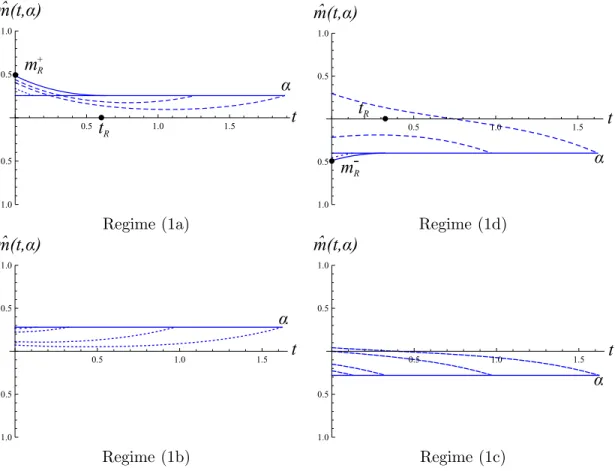
Fore fixed (J, h) and α we say that there is (See Fig. 3):
• No bifurcation if ∆t,α ={mˆ(t, α)}, for all t≥0 and the map t7→mˆ(t, α) is continuous on [0,∞).
• Bifurcation when there exists a 0< tB<∞ such thatt7→mˆ(t, α) continuous except at
t=tB and |∆tB,α|= 2.
• Double bifurcation if there exist times 0< sB< tB <∞ such thatt7→mˆ(t, α) continu-ous except at t=tB andt=sB, and |∆sB,α|=|∆tB,α|= 2.
• Trifurcation if there exists a 0< tT <∞ such that t7→ mˆ(t, α) is continuous except at
t=tT and |∆tT,α|= 3.
The bifurcation times tB and sB, the trifurcation timetT and the trifurcation magnetization
MT (defined below) all depend onJ, h.
Ct,α
m
^ m2
^ m1
,tB
Ct,α
m
,tB ,sB
^ m2
^ m1
^
m3 m^4
Ct,α
m ,tB
^
m1 m^2 m^
Bifurcation Double bifurcation Trifurcation
Figure 3: Different scenarios for the evolution in time of m7→Ct,α(m). Drawn lines: t=tB,
t=tB, sB,t=tT (times at which multiple global minima occur or, equivalently, discontinuity points of t7→mˆ(t, α)). Dotted lines: earlier time. Dashed lines: later time.
The following theorem summarizes the behaviour of ∆t,α (and therefore of the minimizing trajectories ˆϕt,α) for differentt, α. ForJ > 32, let
F(m) := mk
′J,h(m)−kJ,h(m) csch[arccoth(k′J,h(m))],
UB =UB(J, h) := max
m∈[0,1]F(m),
LB =LB(J, h) := min
m∈[−1,0]F(m).
(1.40)
Theorem 1.9. (See Figs. 3–4.)
(1) Suppose that kJ,h(α)6= 0.
(1a) If kJ,h(α)>0 and α >0, then there are m+
R>0 and tR=tR(m +
calculable from (3.8)) such that t 7→ mˆ(t) is strictly increasing on [0, tR] and strictly
decreasing on[tR,∞) with mˆ(tR) =m+R> m∞.
(1b) If kJ,h(α)<0 and α >0, then t7→mˆ(t) is strictly decreasing on [0,∞). (1c) If kJ,h(α)>0 andα <0, then t7→mˆ(t) is strictly increasing on [0,∞).
(1d) If kJ,h(α)<0 and α <0, then there are m−
R>0 and tR=tR(m −
R)>0 (implicitly
calculable from (3.9)) such that t 7→ mˆ(t) is strictly decreasing on [0, tR] and strictly
increasing on[tR,∞) with mˆ(tR) =m−R< α.
In all casesmˆ(0) =α and limt→∞mˆ(t) =m∞.
(2) Suppose that h= 0.
(2a) If 0< J ≤1, then there is no bifurcation.
(2b) If 1< J ≤ 3
2, then there is bifurcation only for α= 0.
(2c) If J > 32, then there is bifurcation if α∈(−UB, UB) and no bifurcation otherwise.
(3) Suppose that h >0.
(3a) If 0< J ≤1, then there is no bifurcation.
(3b) If 1 < J ≤ 32, then there is bifurcation for α ∈ [−1, UB) and no bifurcation for
α∈[UB,1].
(3c) If J > 32, then there exists a h∗ =h∗(J)>0 such that
- for every0< h < h∗ there exists aMT ∈(LB, UB) withMT <0such that there is
* no bifurcation forα∈[UB,1],
* bifurcation for α∈(MT, UB),
* trifurcation for α=MT,
* double bifurcation forα ∈(LB, MT),
* bifurcation for α∈[−1, LB].
- for everyh≥h∗ the behavior is the same as in (3b).
In all cases α7→ tB(α) is continuous and decreasing and α 7→sB(α) is continuous and
increasing.
Theorem 1.9 gives a complete picture of the bifurcation scenario. Regime (1) —which includes cases with zero and nonzero magnetic field— describes two types of behavior of optimal magnetization trajectories: monotone trajectories [cases (1b) and (1c)] and trajectories with
overshoot [cases (1a) and (1d)]. In the latter, ˆm(t) increases to some magnetization m+Rlarger (m−Rsmaller) thanm∞ and afterwards decreases (increases) tom∞. Regimes (2)and (3) refer
to the existence of bifurcations and trifurcations. We observe that the different bifurcation behaviors —no bifurcation, single and double bifurcation— hold for whole intervals of the conditioning magnetization. In contrast, trifurcation appears at a single final magnetization for each h6= 0.
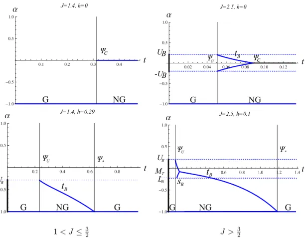
1.5.5 Gibbs versus non-Gibbs
Theorem 1.6 establishes the equivalence of bifurcation and discontinuity of specifications, as proposed in the program put forward in [3]. Due to this equivalence, the following corollary provides a full characterization of the different Gibbs–nonGibbs scenarios appearing during the infinite-temperature evolution of the Curie-Weiss model. Let
0.5 1.0 1.5
1.0 0.5 0.5 1.0
t
t
Rm
+ Rm(t,α)
ˆ
α
0.5 1.0 1.5
1.0 0.5 0.5 1.0
α
t
m-
Rt
Rm(t,α)
ˆ
Regime (1a) Regime (1d)
0.5 1.0 1.5
1.0 0.5 0.5 1.0
α
t
m(t,α)
ˆ
0.5 1.0 1.5
1.0 0.5 0.5 1.0
m(t,α)
ˆ
α
t
Regime (1b) Regime (1c)
Figure 4: Different regimes of Theorem 1.9. Evolution in time of the minimizing trajectories
Corollary 1.10. (See Fig. 5.) (1) Let h= 0.
(1a) If 0< J ≤1, the evolved measure µt is Gibbs for all t≥0.
(1b) If 1< J ≤ 32, then µt is
- Gibbs for0≤t≤Ψc,
- non-Gibbs for t >Ψc with Dt={0}. (1c) If J > 32, then µt is
- Gibbs for0≤t≤ΨU,
- non-Gibbs for t >ΨU with
* Dt={±α} for some α∈(−UB, UB) if ΨU < t <Ψc,
* Dt={0} ift≥Ψc. (2) Let h >0.
(2a) If 0< J ≤1, then µt is Gibbs for t≥0.
(2b) If 1< J ≤ 32, then µt is
- Gibbs for0≤t≤ΨU,
- non-Gibbs for ΨU < t≤Ψ∗ withDt={α} for some α∈[−1, UB),
- Gibbs fort >Ψ∗.
(2c) If J > 32 and h < h∗ small enough, thenµ
t is
- Gibbs for0≤t≤ΨU,
- non-Gibbs for ΨU < t≤Ψ∗ with
* Dt={α} for some α∈[MB, UB) if ΨU < t≤ΨL,
* Dt={α1, α2} for some α1, α2 ∈(LB, MB) if ΨL< t <ΨT,
* Dt={α} for some α∈[−1, MT]if ΨT ≤t≤Ψ∗.
- Gibbs fort >Ψ∗. If h≥h∗, then the behaviour is as in (2b).
In all cases α1, α2, α depend on (t, J, h).
2
Proof of Proposition 1.5 and Theorems 1.6–1.8
Proposition 1.5 is proven in Section 2.1, Theorems 1.6–1.8 are proven in Sections 2.2–2.4.
2.1 Proof of Proposition 1.5
Proof. First note that, by (1.14),
inf ϕ:ϕ(t)=αI
t(ϕ) = inf
m∈[−1,+1]
IS(m) +ϕ: ϕinf(0)=m, ϕ(t)=α
IDt (ϕ)
. (2.1)
It follows from (1.14–1.15) and the calculus of variations that the stationary points of the right-hand side of (2.1) are given by the Euler-Lagrange equation, complemented with a free-left-end condition and a fixed-right-end condition:
∂ ∂s
∂L
∂m˙ (ϕ(s),ϕ˙(s)) = ∂L
∂m(ϕ(s),ϕ˙(s)), s∈ (0, t), ∂L
∂m˙ (ϕ(s),ϕ˙(s))
s=0=
∂IS
∂m(ϕ(s))
s=0,
ϕ(t) =α.
Ψc J=1.4, h=0
t
J=2.5, h=0
t Ψc
t
BΨU
UB
-UB
J=1.4, h=0.29
t
Ψ* ΨU
UB
t
BJ=2.5, h=0.1
t
ΨU Ψ*
UB
M T L
B
t
Bs
B1< J ≤ 32 J > 32
Figure 5: Summary of Corollary 1.10: Time versus bad magnetizations for different regimes. On the vertical α-axis, indicated by a thick line, is the set of bad magnetizations. G=Gibbs, NG=non-Gibbs.
The first and the third equation in (2.2) come from the third infimum in (2.1) and, together with (1.16), determine the form (1.28) of the stationary trajectory. Inserting this form into (1.14) we identify
It( ˆϕmt,α) = Ct,α(m), (2.3)
as stated in (1.25)–(1.26). This identity reduces (1.19) to a one-dimensional variational prob-lem,
inf ϕ: ϕ(t)=αI
t(ϕ) = inf m∈[−1,+1]I
t( ˆϕm
t,α) = inf
m∈[−1,+1]Ct,α(m) (2.4)
The second equation in (2.2) corresponds to the second infimum in (2.1) or, equivalently, to the rightmost infima in (2.4). It gives a trade-off between the static and the dynamic cost, establishing a relation between the initial magnetization and the initial derivative. After some manipulations this equation can be written in the form
−1 2q =a
J(m) cosh(2h) +bJ(m) sinh(2h), m= ˆϕm
t,α(0), q = ˙ˆϕmt,α(0). (2.5)
Differentiating (1.28), we get
˙ˆ
ϕmt,α(s) = 2 csch(2t)
n
and eliminatingq from the last identity in (2.5) in favor oftand α, we conclude that mmust be a solution of (1.22). Imposing this restriction to the chain of identities (2.4) we obtain (1.27) and hence (1.28)–(1.29).
From now on our arguments rely on the study of (1.22), combined with continuity prop-erties ofCt,α as a function oft, α.
2.2 Proof of Theorem 1.6
Equation (1.20) follows in the same way as in the proof of Theorem 2.5 in [7]. Having disposed of this identity, we can now proceed to prove the equivalence. The proof relies on the following lemma.
Lemma 2.1. For any t >0 and α0 ∈[−1,+1], there exists an open neighbourhood Nα0 6=∅
of the later, such that for all α∈ Nα0 \ {α0}
1. Ct,α has only one global minimum, namely, mˆ(t, α).
2. α˜ 7→ mˆ(t,α˜) is continuous at α. If Ct,α0 has a unique global minimum, the continuity
is also valid at α=α0.
3. If Ct,α0 has multiple global minima, for two of them, namely, mˆA(t, α0) and mˆB(t, α0)
lim α↓α0
ˆ
m(t, α) = ˆmA(t, α0) and lim α↑α0
ˆ
m(t, α) = ˆmB(t, α0).
Proof. A straightforward study of (1.22) shows thatCt,α has a finite number of critical points, for every fixed choice ofJ, h, t, α.
Clearly, α 7→ Ct,α and α 7→ lt,α are continuous with respect to the infinity norm in
C([−1,+1],R). This, together with the fact that the left-hand side of (1.22) does not depend on α, implies continuity of any critical point with respect toα.
Let ˆmi(t, α0), i = 1, . . . , v be the global minima of Ct,α0. By continuity of the critical points, there exists a neighbourhood Neα0 and smooth functions Neα0 ∋ α 7→ mi(t, α), i = 1, . . . , v, such that
i. mi(t, α) are local minima of Ct,α,
ii. lim α→α0
mi(t, α) = ˆmi(t, α0).
This properties proves the lemma if v= 1. Otherwise, let
Bi(α) :=Ct,α(mi(t, α)).
The minimal cost is attained at the smallest of them:
Ct,α( ˆm(t, α)) = min
i Bi(α).
Note that there is coincidence at α0 due to the assumed multiplicity of minima:
B(α0) := Bi(α0) , i= 1, . . . v . (2.7)
We expand the functions Bi up to first order order
and observe that,
Bi′(α0)6=Bj′(α0), i6=j. (2.9)
The latter is due to the strict monotonicity of ∂Ct,α
∂α and the fact that each mi(t, α) is a critical points of the function Ct,α(·). From (2.2)–(2.9) we conclude that forα in a possibly smaller neighbourhoodNα0 ⊆Neα0 there is a unique global minimum, and that property 3.holds with
a= arg min i B
′
i(α0), b= arg max i B
′ i(α0),
and
ˆ
mA(t, α0) := ˆma(t, α0), mˆB(t, α0) := ˆmb(t, α0).
We are ready to prove Theorem 1.6.
Proof. Suppose that Ct,α0 has a unique minimizer, denoted by ˆm(t, α0) and let Nα0 be the neighbourhood of the previous lemma. Then (1.21) holds for everyα∈ Nα0, and the continuity of m7→Γt(z, m) for every t, z gives the desired continuity ofα 7→γt(· |α) at α=α0.
To prove necessity, assume that Ct,α0 has multiple global minima. Consider ˆmA and ˆmB as in the previous lemma. Then, we have that there exist sequencesα−n < α0 < α+n converging to α0 and such thatγt(· |α±n) = Γt(·,mˆ(t, α±n)) and
lim
n→∞mˆ(t, α −
n) = ˆmB(t, α0)6= ˆmA(t, α0) = lim
n→∞mˆ(t, α +
n). (2.10)
Again using continuity of Γt with respect tom, we get
lim
n→∞γt(z|α −
n) = Γt(z,mˆB(t, α0))6= Γt(z,mˆA(t, α0)) = limn
→∞γt(z|α + n).
Hence α0 is a bad magnetization.
2.3 Proof of Theorem 1.7
To determine which solutions of (1.22) are global minima of Ct,0 when h= 0, we will pursue
the following strategy. Using (1.22) we can writet as a function ofm:
t(m) := 12arccoth
aJ(m)
m
. (2.11)
This allows us to determine for which timetthe magnetizationm can be apossible minimum
(i.e., a solution of (1.22)).
Lemma 2.2. Let A⊆ [−1,+1] be the set of m-values such that m is the solution of (1.22)
for some t >0, i.e., A={m∈[−1,+1] : aJ(m)/m >1}. Then, for every m∈A,
Ct(m),0(m) = 12Jm2+12log [1−mtanh(Jm)] =:CM(m). (2.12)
In words, (2.12) is the cost for m at the time at which it is a possible minimum.
We now start the proof of Theorem 1.7.
Proof. First note thatlt,0 is linear with slope coth(2t)∈(1,∞) andlt,0(0) = 0, and thataJ is
antisymmetric. Hence, if m is a solution of (1.22), then also−m is a solution. Further note that
aJ′(m) = (2J −1) cosh(2Jm)−2Jmsinh(2Jm),
aJ′′(m) = 4J(J−1) sinh(2Jm)−4J2mcosh(2Jm). (2.13)
(i) If 0< J < 12, then aJ′(m) <0 for all m, and hence m = 0 is the unique solution for all
t > 0. If 12 ≤ J ≤ 1, then aJ′′(m) < 0 for all m, hence aJ is convex, and so it suffices to
compare slopes at 0: kJ,0′(0) =aJ′(0) = 2J−1<1 andl
t,0′(0) = coth(2t)>1. Again, m= 0
is the unique solution for all t >0 (see Fig. 6).
(ii) As before, aJ′′(m) < 0 for all m, but now the slopes at 0 can be equal, which occurs when t = Ψc with Ψc defined in (1.36). This proves that ∆t = {0} for 0 < t ≤ Ψc and ∆t ⊆ {−mˆ(t),0,mˆ(t)} = the set of solutions of (1.22) for t > Ψc. It is easily seen from Fig. 7(a) that ˆm(t) is continuous and strictly increasing on [Ψc,∞) and ˆm(Ψc) = 0. It remains to show that{−mˆ(t),mˆ(t)} are the global minima for all t >Ψc. This follows from the strategy behind the proof of Lemma 2.2. SinceCt,0(0) = 0 for allt >0, it suffices to prove
thatm7→CM(m) is strictly decreasing. From (2.12) we have
CM′ (m) = ∂Ct(m),0
∂m (m) +
∂Ct(m),0
∂t (m)t
′(m). (2.14)
The first term is zero by the definition of t(m) (each m is a stationary point of Ct,0 at time
t=t(m)). The second term is <0 becauset′(m)>0 and
∂Ct,0
∂t (m) =L( ˆϕ
m
t,0(t),ϕ˙ˆmt,0(t))
+ t
Z
0
" ∂L
∂m ϕˆ
m
t,0(s),ϕ˙ˆmt,0(s)
∂ϕˆm t,0
∂t (s) +
∂L ∂m˙ ϕˆ
m
t,0(s),ϕ˙ˆmt,0(s)
∂ϕ˙ˆm t,0
∂t (s) #
ds
=L(0,ϕ˙ˆmt,0(t)) + t
Z
0
∂ ∂s
∂L ∂m˙ ϕˆ
m
t,0(s),ϕ˙ˆmt,0(s)
∂ϕˆm t,0
∂t (s)
ds
=L(0, r)− ∂L
∂m˙ (0, r)r =−12p4 +r2+ 1<0
(2.15) withr= ˙ˆϕm
t,0(t), where the second equality uses (2.2). SinceCM(0) = 0, this yields the claim (see Figs. 7(a),7(b),7(c)).
(iii) This case is more difficult, becauseaJ no longer is convex on (0,1). Let Ψ1
c be the first time at which a solution different from 0 exists. To identify Ψ1c, let
Tm(x) := (x−m)aJ ′
and let m1 be the solution of the equation Tm1(0) = 0 =−m1a J′(m
1) +aJ(m1), i.e.,
m1 =
aJ(m 1)
aJ′(m 1)
. (2.17)
From m1 we get t1c by using (2.11): t1c =t(m1). As before, a solution of (1.22) for t≥t1c is not necessarily a minimum. To find out when it is, we follow the same strategy as in case (ii). Again,Ct,0(0) = 0 for all t >0, and hence we must look for m∗ >0 such that
CM(m∗) = 0. (2.18)
Knowing m∗, we are able to compute Ψc using (2.11),
t∗ =t(m∗). (2.19)
In words,t∗ is the first time at which 0 no longer is a minimum. As in case (ii), it suffices to
prove that m7→CM(m) is strictly decreasing on (m∗,∞). Again, we have (2.14). Since
t′(m) =1
2(arctanh)
′
aJ(m)
m a
J′(m)−aJ(m)
m
1
m, (2.20)
it follows that t′(m) = 0 if and only of m = aJ(m)/aJ′(m), which is the same condition as (2.17). This gives us a graphical argument to conclude that t′(m)< 0 for 0< m < m
1 and
t′(m)>0 for m > m1 (see Figs. 7(d),7(e),7(f)). On the other hand,m∗ > m1.
J=0.4
J=0.9
m
Figure 6: m7→aJ(m),m7→l
t,0(m) for Regime (i).
2.4 Proof of Theorem 1.8
Proof. From (1.28) it follows that
˜
m > m,˜t > t =⇒ ϕˆm˜t,˜0(s)>ϕˆmt,0(s) ∀0≤s≤t. (2.21)
(i) First note that, because CM(m∗) = 0,
∂m∗
∂J =−
∂CM
∂J (m∗)
∂CM
∂m (m∗)
m
(a)
m Ct,0(m)
(b)
m CM(m)
(c)
Regime (ii),J = 1.3.
m m1 m*
(d)
m Ct,0(m)
m
(e)
m CM(m)
m
(f)
Regime (iii), J = 2.
Figure 7: (a+d) m 7→ aJ(m), m 7→ l
t,0(m); (b+e) m 7→ Ct,0(m), for 0 ≤ t < Ψc (dotted),
t= Ψc (drawn), t >Ψc (dashed); (c+f)m 7→CM(m).
As in Section 2.3, case (iii), we have (∂CM/∂m)(m∗)<0. But
∂CM
∂J (m∗)>0 ⇐⇒ m∗<tanh(Jm∗), (2.23) which yields the claim becausem∗< m∞.
(ii) The claim is straightforward for 1< J ≤ 32. ForJ > 32 we need to prove that the function
J →aJ(m∗)/m∗ is strictly increasing. In fact,
∂ ∂J
aJ(m
∗)
m∗
= 1
m2
∗
−∂m∗
∂J
aJ(m∗)−m∗
∂aJ
∂m(m∗)
+m∗
∂aJ
∂J (m∗)
= 1 + cosh(2Jm∗)−m∗sinh(2Jm∗).
(2.24)
The strict positivity of the last expression is equivalent to the inequality m∗ < coth(Jm∗),
which is satisfied forJ >1.
(iii) We haveaJ(m)↓a32(m) asJ ↓ 3
2 for allm∈(0,1), withaJ anda 3
2 continuous. By Dini’s theorem, the convergence is uniform.
(iv) Since Ψc( ˜J)<Ψc(32), the same argument as in case (iii) can be used.
(v) and (vi) are consequences of parts (ii) and (iii) of Theorem 1.7.
3
Proof of Theorem 1.9
3.1 Regime (1): Overshoots
The trick is again to write tas a function of m. From (1.22), we have
−kJ,h(m) + 2mcoth(2t) =mcoth(2t) +αcsch(2t). (3.1)
Hence, from (1.23),
kJ,h(m)[−kJ,h(m) + 2mcoth(2t)]
= [mcoth(2t)−αcsch(2t)] [mcoth(2t) +αcsch(2t)] (3.2)
which implies
−kJ,h(m)2−α2 = (m2−α2) coth2(2t)−2mkJ,h(m) coth(2t). (3.3)
Solving for twe find
tF(m) :=
1 2arccoth
mkJ,h(m) +|α|pΦ(m)
m2−α2
if m6=±α
1
2arccoth
kJ,h(m)2+m2
2m kJ,h(m)
if m=±α , m kJ,h(m)<0
0 if m=±α , m kJ,h(m)>0
(3.4)
tL(m) :=
1 2arccoth
mkJ,h(m)− |α|pΦ(m)
m2−α2
if m6=±α
1
2arccoth
kJ,h(m)2+m2
2m kJ,h(m)
if m=±α , m kJ,h(m)>0
0 if m=±α , m kJ,h(m)<0
(3.5)
with
Φ(m) :=kJ,h(m)2−m2+α2. (3.6) These are times at whichmis a stationary point (not necessarily a minimum) both forCt,α(m) and forCt,−α(m) [Equation (3.2), and hence the solutions (3.4) are insensitive to the sign of
α]. Overshoots and undershoots occur for values ofm satisfying (i)tF(m)>0 andtL(m)>0 and (ii) at these times m is a minimum.
Them-dependence oftF andtLis depicted in Figs 8 and 9 for cases in which both functions are injective, i.e., for α for which there is only one critical point for each t. In more complicated cases, for instance, when overshoot and bifurcation occur simultaneously, there are two or more stationary points only one of which is a minimum.
We divide the analysis in four steps.
Step A: Existence of z+, z− and z−+. We observe that there exists a uniquem∞>0 such
that kJ,h(m∞) =m∞. Furthermore,
kJ,h(m) = 0 ⇐⇒ tanh(2h) = −a J(m)
bJ(m) =:A(m). (3.7)
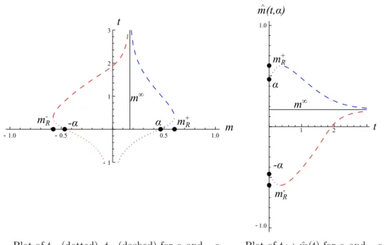
-1.0 1.0
1 2
m^(t,α)
t m+R
m-R
α
m∞
-α
-1.0 -0.5 0.5 1.0
-1 1 2 3
m
t
m+R
m-R α
m∞
-α
Plot oftF (dotted),tL (dashed) forαand−α. Plot oft7→mˆ(t) forαand−α.
Figure 8: Overshoot for (J, h, α) in Regime (1a) or for (J, h,−α) in Regime (1d). Parameters: (J, h) = (0.95,0.01), α= 0.46.
-1.0 -0.5 0.5 1.0
1 2 t
α
-α
m∞ m^(t,α)
m t
α -α
m∞
Plot oftF (dotted),tL (dashed) forαand−α. Plot oft7→mˆ(t, α) forαand−α.
m
A(m)
z- z-+
z+
Figure 10: Plot of A and intersection with the constant tanh(2h).
exists a unique z+ = z+(J, h) > 0 such that kJ,h(z+) = 0 and, in addition, if tanh(2h) <
max
m∈[−1,0]A(m), then there exist−1 < z
− < z−+<0 such that kJ,h(z−) =kJ,h(z−+) = 0 (see
Fig. 10).
Step B:Existence of m+R, m−R and relation between m∞ and α.
(Ba) Existence of m+R: kJ,h(α) > 0 together with α > 0 and Step A imply α < z+. Since Φ(α)>0 and Φ(z+)<0, it follows that there exists am+R such that 0< α < m+R< z+ and
Φ(m+R) = 0. (3.8)
The latter in turn implies that kJ,h(m+
R)2 = m+ 2
R −α2. This, together with kJ,h(m+R) > 0, implies thatkJ,h(m+R)< m+R, which leads to m∞< m+R.
(Bd) Existence of m−R: As in (Ba), Φ(z−) < 0 and Φ(α) > 0 imply that there exists a m−R such that z−< m−R< α <0 and
Φ(m−R) = 0. (3.9)
(Bc): kJ,h(α) >0 and α < 0 imply α < m
∞. This follows from the fact that kJ,h(α) > α
implies α < m∞ by (1.33).
(Bb): kJ,h(α)<0 and α >0 imply α > m
∞. Again, this is a consequence of (1.33).
Step C:Consequence of the positivity of times. Only positive solutions of Equation (3.4) are
of interest. This implies the constraints
tF(m)>0 ⇐⇒ ηF(m) :=m kJ,h(m) + (α2−m2) +|α|
p
Φ(m)
(
>0 ifm2> α2,
<0 ifm2< α2, (3.10)
and
tL(m)>0 ⇐⇒ ηL(m) :=m kJ,h(m) + (α2−m2)− |α|
p
Φ(m)
(
>0 ifm2> α2,
<0 ifm2< α2. (3.11)
The functionsηF andηL satisfy
ηF(α) =αkJ,h(α) +|α||kJ,h(α)|=
(
>0 if α kJ,h(α)>0,
ηL(α) =αkJ,h(α)− |α||kJ,h(α)|=
(
= 0 if α kJ,h(α)>0,
<0 ifα kJ,h(α)<0. (3.13)
Also, from (1.33),
ηF(m∞) = 2|α|2, η′F(m∞) = 2m∞kJ,h′(m∞),
ηL(m∞) = 0, η′L(m∞) = 0.
(3.14)
Last line implies that m∞ is a root of ηL but there is no change of sign around it. Finally, from expressions (3.10)-(3.14) we conclude that:
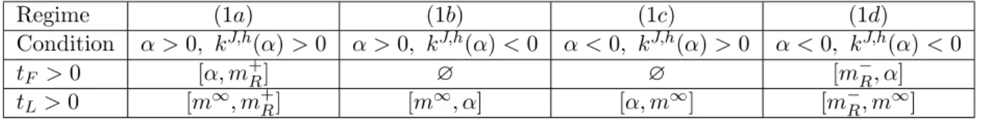
• The zeros ofηF, ηL are a subset of{m∞,±α}.
• The intervals in whichηF and ηL satisfies the constrains (3.10)-(3.11) are:
Regime (1a) (1b) (1c) (1d)
Condition α >0, kJ,h(α)>0 α >0, kJ,h(α)<0 α <0, kJ,h(α)>0 α <0, kJ,h(α)<0
tF >0 [α, m+R] ∅ ∅ [m−R, α]
tL>0 [m∞, m+R] [m∞, α] [α, m∞] [m−R, m∞]
We observe that in regime (1a) each value ofm∈[α∧m∞, m+R] is attained at two different timestF (“First”) andtL(“Last”). The same happens in regime (1d) form∈[mR−, α∨m∞].
These phenomena correspond respectively, to an over and an under shoot. The proof is completed by showing that the trajectories have the right monotonicity properties.
-1.0 -0.5 0.0 0.5 1.0
0.1 0.2 0.3
0.4
m
m-R m+
R
m m+R
m-R
α m∞
-α
Figure 11: ηF (dotted) andηL(dashed) for (J, h, α) in regime 1(a) and for (J, h,−α) in regime 1(d). Parameters: (J, h) = (0.95,0.01), α= 0.46 as in Fig. 8.
Step D:Monotonicity.
By using implicit derivation we get
∂mˆ ∂t (t) =
∂lt,α
∂t ( ˆm) [kJ,h]′( ˆm)−l′
t,α( ˆm) =
2 csch(2t)nmˆ csch(2t)−αcoth(2t)o
[kJ,h]′( ˆm)−coth(2t) . (3.15)
On the other hand, if ˆm = ˆm(t) is a critical point kJ,h( ˆm) = l t,α( ˆm)
∂mˆ
∂t (t) = 0 ⇐⇒ Φ( ˆm(t)) = 0.
Splitting in cases according to different values of ˆm, it is not hard to conclude from (3.8) and (3.15) the following monotonicity properties of the trajectories.
Regime (1a) (1b) (1c) (1d)
ˆ
m incr. 0< t < t(m+R) ∅ 0< t <∞ t(m−
R)< t <∞ ˆ
m decr. t(m+R)< t <∞ 0< t <∞ ∅ 0< t < t(m−
R)
This concludes the proof of part 1 of Theorem 1.9.
3.2 Bifurcation
Bifurcation proofs rely on the following facts.
(B1) For short times there is a unique critical point, close toα.
(B2) Therefore, in order for bifurcation to occur a local maximum and a local minimum must appear in the course of time. Given condition (1.22), usual arguments imply that two (or more) stationary points appear at times larger than ˜t if the curves l˜t,α and kJ,h become tangent at a certain magnetization ˜m. The pairs ( ˜m,˜t) are determined by the following two equations (a similar argument was used in the proof of Theorem 1.7(iii)):
kJ,h′( ˜m) = coth(2˜t),
kJ,h( ˜m) = ˜mcoth(2˜t)−αcsch(2˜t). (3.16)
Inserting the first equation into the second, we get
F( ˜m) := m˜
kJ,h′( ˜m)−kJ,h( ˜m)
cscharccoth kJ,h′( ˜m) =α. (3.17)
We are left with the task of determining whether or not this equation has solutions. Note that
F′(m) = 0 ⇐⇒ kJ,h′′(m) = 0 or m=kJ,h(m)kJ,h′(m). (3.18)
In what follows all the assertions about F can be checked by using the equivalence in (3.18) and doing a straightforward analysis of kJ,h.
(B3) t7→Ct,α is continuous with respect to k · k∞. Hence, when a new minimum appears it
cannot be a global one. Both α7→Ct,α and h7→Ct,α are also continuous.
Whenever a local maximum/local minimum appears (disappears), we will refer to this behaviour as LMLMA (LMLMD). We proceed by looking at h= 0 andh6= 0 separately.
Part (2) (h = 0, see Fig. 12). The scenario for α = 0 has already been proven in Theorem
1.7. We concentrate onα >0; this is no loss of generality due to the antisymmetry ofF.
Claim: Whenever α >0, negative solutions of (3.17) can not cause bifurcations. In fact, let tnc be the time at which the critical point in the negative side emerge. Let also,
d(t) :=Ct,α(m−(t, α))−Ct,α( ˆm(t, α)), t≥tnc,
where m−(t, α) is the negative local [because of (B3)] minimum and ˆm(t, α) is the global
minimum of Ct,α. The last one is positive due to (B1). and the supposition of α > 0. By definition,d(tnc)>0 and by (B4) limt→∞d(t) = 0. Doing calculations similar to (2.15) and
using that m−(t, α), ˆm(t, α) are both critical points, we get that d′(t) < 0 ∀ t > tnc. This proves the claim.
In what follows we focus in equation (3.17). Owing to the previous claim, in order to bifurcation to occur a positive solution of (3.17) is needed.
(2a-b) If 0 < J ≤ 32, then F′(m) < 0 for all m ∈ (−1,+1). Hence, for all α > 0 there is only one solution of (3.17). This solution turns out to be negative and hence it can not correspond to a bifurcation.
(2c) If J > 32, F has only one global maximum on the positive side, with value UB =
UB(J) > 0. Combining B1.-B4., we get that there is bifurcation if and only if α ∈ [0, UB] = Im(F|[0,1]).
Part (3)(h >0, see Fig. 13).
Remark: Ifh >0, thenB4. (Symmetry breaking) allows the appearance of solutions of (3.17) leading to bifurcations.
Once more, let study the different scenarios for F whenh >0.
(3a) If 0< J ≤1, then Im(F)⊆[−1,+1]c. Therefore (3.17) has no solution for any |α| ≤1 and there is no bifurcation.
(3b) If 1< J ≤ 3
2, thenF has a unique maximum form∈[0,1] with valueUB=UB(J, h)<0,
and [−1, UB] = Im(F|[0,1]). Arguing as in the claim of Part 2 for α > UB, we conclude that there is bifurcation if and only if α∈[−1, UB].
(3c) AssumeJ > 32.
1. For h > 0 small enough the behaviour is “close” to the h = 0 case due to the continuity of h7→Ct,α with respect to the infinite norm.
Indeed, there exists LB := min[−1,0]F ≈ −UB(J,0) and UB := max[0,1]F ≈
UB(J,0), with (−1, UB] = Im(F|[0,1]). There are different regimes forα:
(a) For α < LB, there is a unique solution of (3.17), which is in the positive side, leading to a bifurcation [because of (B4) ].
-1.0 -0.5 0.5 1.0
-1.0
-0.5 0.5 1.0
F
m
m∞
-m∞
α
-1.0 -0.5 0.5 1.0
-1.0
-0.5 0.5 1.0
F
m
α
UB
-UB
m∞
-m∞
-1.0 -0.5 0.5 1.0
-0.02 0.02
0.04
0.06
Ct,α(m)
(1) (2)
(3)
m
α
m∞
-m∞ d(t
nc) m―-(tnc,α)
mˆ (tnc,α)
-1.0 -0.5 0.5 1.0
-0.3
-0.2
-0.1 0.1 0.2 0.3 (1)
(3) Ct,α(m)
m
m∞
α
(2)
-m∞
Regime (2a-b), J = 1.15, h= 0 Regime (2c),J = 2.5, h= 0.
Figure 12: First row: Plot of m 7→ F(m). = LMLMA not leading to bifurcation; N = LMLMD; = LMLMA leading to bifurcation; ⋆ = bifurcation . Second row: Plot of m7→Ct,α(m) for different times. Short time (dotted) bifurcation (solid), long time (dashed).
(c) For 0< α / UB there is LMLMA on the positive and negative sides. As in theh= 0 case, the negative one does not lead to a bifurcation, and thus only one bifurcation occurs, which happens to be in the positive side.
(d) By the continuity property(B3) and the monotonicity of α7→sB(α) (proved below) , the two previous regimes coalesce, leading to an intermediate value MT ∈(LB, UB) such that trifurcation occurs at α=MT.
(e) For α > UB there is no positive solution to (3.17) with α ∈ [0,1]. Hence, no bifurcation occurs.
2. The limit h→ ∞in (3.17) yields
maJ′(m) +bJ′(m)−aJ(m) +bJ(m)
aJ′(m) +bJ′(m) =α.
Hence, for h > 0 large enough we get a behaviour similar to (3b), but with UB(J, h)>0.
-1.0 -0.5 0.5 1.0
-1.0
-0.5 0.5 1.0
F
m m∞
UB -1.0 -0.5 0.5 1.0
-1.0
-0.5 0.5 1.0
F
m m∞
UB
(3b), h small, J = 1.42,h= 0.15 (3b), h large, J = 1.42, h= 1.6
-1.0
1.0
-1.0 0.5 1.0
UB F
m
LB MT
αB
αDB
(a) (b) (c) (d) (e)
-1.0 -0.5 0.5 1.0
-1.0
-0.5 1.0
F
m m∞
UB
(3c), h small, J = 2.9,h= 0.15 (3c), h large, J = 2.9, h= 1.6
Figure 13: Plot of m 7→ F(m) for different regimes of J when h > 0. = LMLMA not causing a bifurcation; N= LMLMD;= LMLMA causing a bifurcation.
3.2.1 Monotonicity of the functions tB(α) and sB(α)
The bifurcation times are characterized by the following equations:
kJ,h( ˆm
1) = ltB,α( ˆm1), kJ,h( ˆm
2) = ltB,α( ˆm2), CtB,α( ˆm1) = CtB,α( ˆm2).
(3.19)
The first two equations say that ˆm1 and ˆm2 are stationary points at the same timetB, while the third one establishes the equality of costs at this time tB. Taking the derivative with respect to α of the third equation we get
∂tB
∂α =−
∂CtB,α
∂α ( ˆm2)−
∂CtB,α
∂α ( ˆm1)
∂CtB,α ∂tB
( ˆm2)−
∂CtB,α
∂tB
( ˆm1)
. (3.20)
A straightforward computation using the first two equations shows that ∂tB
∂α <0, which implies that α 7→ tB(α) is continuous and decreasing. A similar argument shows that α 7→sB(α) is continuous and increasing.
References
[2] A.C.D. van Enter, R. Fern´andez, F. den Hollander and F. Redig, Possible loss and recov-ery of Gibbsianness during the stochastic evolution of Gibbs measures, Commun. Math. Phys. 226 (2002) 101–130.
[3] A.C.D. van Enter, R. Fern´andez, F. den Hollander and F. Redig, A large-deviation view on dynamical Gibbs-non-Gibbs transitions, Moscow Math. J. 10 (2010) 687–711.
[4] A.C.D. van Enter, C. K¨ulske, A.A. Opoku and W.M. Ruszel, Gibbs-non-Gibbs properties forn-vector lattice and mean-field models, Braz. J. Prob. Stat., 24 (2010) 226–255.
[5] A.C.D. van Enter and W.M. Ruszel, Loss and recovery of Gibbsianness for XY spins in a small external field, J. Math. Phys. 49 (2008) 125208.
[6] A.C.D. van Enter and W.M. Ruszel, Gibbsianness versus non-Gibbsianness of time-evolved planar rotor models, Stoch. Proc. Appl. 119 (2010) 1866–1888.
[7] V. Ermolaev and C. K¨ulske, Low-temperature dynamics of the Curie-Weiss model: Peri-odic orbits, multiple histories, and loss of Gibbsianness, J. Stat. Phys. 141 (2010) 727–756.
[8] F. den Hollander, Large Deviations, Fields Institute Monographs 14, American Mathe-matical Society, Providence, RI, 2000.
[9] C. K¨ulske and A. Le Ny, Spin-flip dynamics of the Curie-Weiss model: Loss of Gibbsian-ness with possibly broken symmetry, Commun. Math. Phys. 271 (2007) 431–454.
[10] C. K¨ulske and A.A. Opoku, The posterior metric and the goodness of Gibbsianness for transforms of Gibbs measures, Elect. J. Prob. 13 (2008) 1307–1344.
[11] C. K¨ulske and A.A. Opoku, Continuous mean-field models: limiting kernels and Gibbs properties of local transforms, J. Math. Phys. 49 (2008) 125215.
[12] C. K¨ulske and F. Redig, Loss without recovery of Gibbsianness during diffusion of con-tinuous spins, Probab. Theory Relat. Fields 135 (2006) 428–456.
[13] A. Le Ny and F. Redig, Short time conservation of Gibbsianness under local stochastic evolutions, J. Stat. Phys. 109 (2002) 1073–1090.
[14] T.M. Liggett, Interacting Particle Systems, Grundlehren der Mathematischen Wis-senschaften 276, Springer, New York, 1985.
[15] A.A. Opoku,On Gibbs Properties of Transforms of Lattice and Mean-Field Systems, PhD thesis, Groningen University, 2009.