Climate-Human Health Vulnerability: Identifying Relationships between Maximum Temperature and Heat-Related Illness across North Carolina, USA
Margaret Mae Kovach
A dissertation submitted to the faculty at the University of North Carolina at Chapel Hill in partial fulfillment of the requirements for the degree of Doctor of Philosophy in the Department
of Geography.
Chapel Hill 2015
iii ABSTRACT
MARGARET M. KOVACH: Climate-Human Health Vulnerability: Identifying Relationships between Maximum Temperature and Heat-Related Illness across North
Carolina (Under the direction of Charles E. Konrad II)
v
ACKNOWLEDGEMENTS
I gratefully acknowledge the patient guidance, direction, and friendship of my advisor, Charles Konrad. His mentorship has had a positive impact on my professional and personal development and challenged me to become the academic I am today. I am grateful to my dissertation committee members: Erika Wise, Michael Emch, Conghe Song, and Kirstin Dow. I am grateful to Christopher Fuhrmann for his mentorship and support throughout my graduate program. I also acknowledge the North Carolina State Climate Office, the Southeastern Regional Climate Center, Carolinas Integrated Sciences and Assessments, National Science Foundation’s Doctoral Dissertation Research Improvement Grant (Award Number: 1434202), and the Environmental Protection Agency’s STAR Fellowship Assistance Agreement (no.
F13D10708). Lastly, I am thankful to my many colleagues and friends too numerous to name.
This data was provided by NC DETECT is a statewide public health syndromic surveillance system, funded by the NC Division of Public Health (NC DPH) Federal Public Health Emergency Preparedness Grant and managed through collaboration between NC DPH and UNC-CH Department of Emergency Medicine’s Carolina Center for Health Informatics. The NC DETECT Data Oversight Committee does not take responsibility for the scientific validity or accuracy of methodology, results, statistical analyses, or conclusions presented.
Outside academia, I am indebted to my parents whose countless scarifies and
vi
vii
TABLE OF CONTENTS
LIST OF TABLES ... ix
LIST OF FIGURES ... x
LIST OF ABBREVIATIONS ... xi
CHAPTER 1: INTRODUCTION ... 1
CHAPTER 2: AREA-LEVEL RISK FACTORS FOR HRI ... 7
Materials and Methods ... 10
Health Data ... 10
Demographic and Socioeconomic Data ... 11
Land Cover and Agricultural Data ... 11
Analysis ... 13
Results ... 19
Discussion ... 21
Conclusion ... 25
CHAPTER 3: RELATIONSHIPS BETWEEN HRI AND TEMPERATURE ... 27
Methods ... 29
Data sources ... 29
Urban and rural character ... 32
Statistical analysis ... 34
Results ... 35
Basic characteristics of HRI across North Carolina ... 35
Regional characteristics of HRI ... 37
Rural and urban characteristics of HRI ... 39
Demographic characteristics of HRI ... 40
Discussion ... 43
Conclusion ... 49
CHAPTER 4: INTRA-SEASONAL RELATIONSHIPS OF HRI ... 51
Data and Methods ... 53
viii
Health data ... 54
Rurality ... 56
Statistical analysis ... 57
Results ... 58
Basic characteristics of HRI across North Carolina ... 58
Regional characteristics of HRI ... 60
Demographic characteristics ... 62
Rural and urban characteristics ... 65
Discussion ... 67
Conclusions ... 73
CHAPTER 5: CONCLUSIONS ... 74
ix
LIST OF TABLES
Table 1: Coefficient of determination and correlation coefficient for potential risk factors of HRI. ... 15
Table 2: Ordinary least regression model output for rural and urban location ... 17
Table 3: Spatial error regression model output ... 18
Table 4: Mean and Standard Deviation of Area-Level Risk Factors ... 20
Table 5: Definition of Rural-Urban Commuting Codes (RUCA codes). ... 34
Table 6: Regional and demographic characteristics of HRI ... 38
Table 7: HRI incidence rates for males and females ... 43
Table 8: Characteristics of rural and urban locations. ... 47
Table 9: 2007 to 2012 Monthly mean maximum, minimum and number of HRI ED visits ... 54
Table 11: Definition of Rural and Urban Locations defined using the RUCA Codes ... 57
Table 12: HRI incidence for the physiographic regions and the state. ... 61
Table 13: HRI incidence for ZIP codes with sweet potato or tobacco acreage ... 62
Table 14: Total HRI Threshold Temperature, Peak Temperature. ... 64
Table 15: Total HRI ED visits per 100,000 person-years ... 66
x
LIST OF FIGURES
Figure 1: Map of study area and heat-related illness rates per 100,000 person-years. ... 19
Figure 2: Maximum Temperature and Heat Index versus Heat-Related Illness ... 32
Figure 4 HRI versus maximum temperature across North Carolina ... 37
Figure 5: Daily HRI ED visits per 100, 000 people for different physiographic regions ... 39
Figure 6: Daily HRI with respect to temperature for different rural-urban regions ... 40
Figure 7: HRI person-years for different age demographics across the rural-urban continuum ... 41
Figure 8: HRI ED visits with respect to maximum temperature for different demographics ... 42
Figure 9: HRI for May through September from 2007 to 2012. ... 58
Figure 10: Daily HRI with respect to temperature. ... 59
Figure 11: Daily HRI with respect to temperature across the(a) Piedmont (b) Coastal Plain ... 61
Figure 12: HRI with respect to maximum temperature for different demographic ... 64
xi
LIST OF ABBREVIATIONS
AIC Akaike Information Criterion
ACS American Community Survey
AC Air Conditioning
ED Emergency department
GAM Generalized Additive Model
GIS Geographic Information System
HRI Heat-related illness
HVI Heat Vulnerability Index
NC North Carolina
NC-DETECT North Carolina Disease Event Tracking and Epidemiologic Collection Tool
NLCD National Land Cover Database
NWS National Weather Service
OLS Ordinary Least Square Multivariate Linear Regression Model
VIF Variance Inflation Factor
WWAMI Washington, Wyoming, Alaska, Montana, and Idaho
ZCTA ZIP code Tabulation Area
1
CHAPTER 1: INTRODUCTION
Environmental heat stress is associated with increased morbidity and mortality. Heat stress occurs when the thermoregulation system is overwhelmed and cannot shed sufficient heat through sweating, causing the body’s core temperature to rise. In such instances, this heat stress
can cause heat-related illness (HRI), which clinically manifests with symptoms, such as heat cramps, heat syncope, and heat exhaustion (Becker and Stewart 2011, Lugo-Amado et al. 2004). Signs of heat-related illness may include fatigue, thirst, tiredness, mental confusion, weakness, paleness, fainting, nausea, vomiting, and headache (Kilbourne et al. 1980). If left untreated, HRI can progress to heat stroke, a life threatening condition, with severe health effects such as, delirium, convulsions, or coma. Survivors of heat stroke experience neurologic impairment, which can persist long after recovery and often results in mortality within one year (Dematte et al. 1998).
2
Kilbourne et al. 1982). Living conditions, including the type of building, floor level, the presence of an air conditioning unit and the number of rooms, were also found to be important determinants of heat-related morality (Semenza et al. 1996). Other literature that examined heat waves in Chicago (1990), St. Louis (1980), and Kansas City (1980) have found similar results with greater mortality among the elderly, poor, social isolated non-whites, and city dwellers (Jones et al.1982, Naughton et al. 2002, Kilbourne et al. 1982).
Despite a well-establish relationship between heat and mortality, few studies have
attempted to assess the impact of heat on morbidity. This gap in research is due to restrictions on the use and availability of hospital and emergency department data. These studies have
contradictory results from heat-mortality studies. In London, for instance, United Kingdom hospital ED visits were compared to overall mortality rates. Results found that for the same high temperatures, ED visits did not increase, whereas mortality increased markedly (Kovats et al. 2004). Similarly, in the Chicago 1995 heat wave, overall mortality increased 147%, whereas ED visits increased by 11% (Semenza et al. 1999, Whitman et al. 1997). However, when examining ED visits specifically related to HRI, there are significant increases with temperature, even with modest temperature increases (Knowlton et al. 2009). Most of these HRI ED admissions occur in the elderly (i.e. 65 years and older), children, or for people with underlying medical
conditions. These populations are generally considered more heat vulnerable, with
thermoregulation systems that do not readily mitigate high temperatures (Jones et al. 1982, Semenza et al. 1999).
Variations in the relationship between temperature and HRI or deaths are complicated by a population’s coping abilities and the timing of the heat onset. In the United States, there is not a
3
(McGeehin and Mirabelli 2001). Kalkstein and Davis (1989) found that the strongest
relationships between temperature and mortality in the United States occur in regions where hot weather is uncommon and the weakest relationships occur in the hottest locations. These differences in the relationship between temperature and mortality can be attributed to regional acclimation (Kalkstein and Davis 1989). Similarly, Curriero et al. (2002) found that residents of northern cities (e.g. Chicago, IL Boston, MA) have lower minimum mortality temperatures than residents of southern cities (e.g. Miami, Tampa, FL). They also confirmed that residents of northern cities are at greater risk of dying from heat events due to a lack of regional acclimation. Research into acclimation demonstrates that initial physiological acclimation to hot
environments can occur over a few days, but complete acclimation may take several years (Zeisberger et al. 1994).
The timing of extreme heat across summer months is also important. Heat waves or high temperatures occurring in the early summer or spring result in more deaths than the same high temperatures in the later summer months. This phenomenon is known as mortality displacement (formerly known as the harvesting effect) and occurs when the most vulnerable populations experience mortality earlier in the summer, while less vulnerable populations survive extreme heat either through behavioral or physiological adaptations (Basu and Samet 2002, Anderson and Bell 2011).
4
1.) Heat-related illness is easily prevented through basic hydration or relocating to a cooler environment; thus basic warning and public health interventions can easily mitigate future heat-health effects.
2.) Meteorologists can accurately forecast the severity, duration, and intensity of heat several days prior to an extreme heat event. Therefore, identifying temperatures that cause HRI will allow for the activation of an early heat warning system or emergency response plan to mitigate future HRI. In other locations, heat warning systems (HWWS) have been applied and shown to decrease mortality (Ebi et al. 2004).
3.) High risk populations experience a disproportionate number of health impacts. Identifying these high risk populations in a given location will allow for targeted public health and resource allocation that can mitigate any negative health impacts. This motivates the need to identify vulnerable locations and populations as well as the temperatures that increase HRI.
The aim of this dissertation is to identify local to regional scale patterns of climate-health vulnerabilities and the temperatures that control these patterns. This will be carried out by identifying the spatiotemporal footprint of HRI and how it intersects with the spatial patterns of temperature. Specifically, this study will address the following questions:
1.) What is the spatial pattern of HRI across North Carolina and how does this pattern relate to socioeconomic, demographic, and land cover patterns?
2.) What is the spatial relationship between temperature and HRI, and how this
5
3.) What is the intra-seasonal relationship between temperature and HRI across the warm months?
This study expands upon previous literature in several ways:
1.) It examines populations that have not been studied in the context of heat-health vulnerability (e.g. rural populations, farm workers). Previous research has focused mainly on metropolitan locations, where population density is the greatest and there is a heat island in which surface heat retention elevates nocturnal temperatures (McGeehin and Mirabelli 2001). This research, complements some recent research (e.g. Sheridan and Dolney 2003, Gabriel and Endlicher 2011), which suggests that rural populations experience greater rates of heat-health effects.
2.) It assesses regional differences in the heat morbidity and temperature relationship across the state of North Carolina. This approach addresses the need for more multi-location studies with consistent methodologies to make comparisons between
temperature effects on locations and populations (Kalkstein and Greene 1997, Ye et al. 2012).
3.) It considers heat vulnerability through an examination of heat morbidity (i.e. HRI) rather than heat mortality. Because heat morbidity has received limited attention, these these findings open the door on that dimension of HRI.
6
2013). The state also provides an excellent setting to study patterns of HRI due to its humid subtropical climate, large and rapidly growing population, and state of the art morbidity surveillance network (i.e. NC-DETECT).
7
CHAPTER 2: AREA-LEVEL RISK FACTORS FOR HRI
Every year, a large number of hospitalizations and deaths occur in association with exposure to heat (Basu and Samet 2002). This exposure is detrimental to a person’s health when it overwhelms their ability to thermoregulate, increasing the likelihood of succumbing to heat stroke or exacerbating pre-existing health conditions (Kovats and Hajat 2008; Luber and McGeehin 2008). Most of these heat-health effects are concentrated in geographic areas where certain socioeconomic factors and physical exposure increase a population’s vulnerability to
heat-related morbidity or mortality. Adverse health effects from heat are preventable through basic hydration or relocating to a cooler environment; therefore, public health interventions are a key component in reducing these effects (Luber and McGeehin 2008).However, establishing which populations are at greatest risk is a complex issue involving a combination of
environmental and social conditions.
8
al. 1999). Most of these morbidities befall the elderly (65 years and older) and individuals with underlying medical conditions (Jones et al. 1982; Semenza et al. 1996, 1999; Knowlton et al. 2009).
The majority of heat-health research has been conducted in urban areas, which are generally warmer than surrounding rural areas due to the urban heat island effect (Dousset et al. 2011; Böhm 1998). Additionally, since urban areas display high population densities, the number of deaths and morbidities attributable to extreme heat can be very high (Luber and McGeehin 2008). Less research has been conducted in rural regions. Some examples include Gabriel and Endlicher (2011), who found higher mortality rates in urban locations compared to rural locations during extreme heat events in Germany. Similar results were noted in and around St. Louis and Kansas City, MO during the 1980 heat wave (Jones et al. 1982). In contrast, both Sheridan and Dolney (2003) and Henderson et al. (2013) found higher mortality rates in rural and suburban regions compared to urban regions in Ohio, USA and British Columbia, Canada, while Lippmann et al. (2013) found a similar pattern in North Carolina, USA using ED visit data for HRI.
Heat-health researchers have also attempted to address heat vulnerability at a local level by aggregating previous established area-level risk factors for heat mortality into heat
9
vulnerability index (HVI). Using principal components analysis, their index reduces 10 variables into four representative factors including social and environmental vulnerability, social isolation, prevalence of air conditioning, and proportion of the population that are elderly or diabetics. Using the HVI, they contrast differences in vulnerability across different metropolitan regions of the United States, particularly downtown metropolitan areas, which have some of the highest HVI values.
The main limitation of these studies is that their results (i.e. identification of areas with high and low heat vulnerability) are not validated with actual counts of morbidity or mortality. Recent research has evaluated some of these indices, including the HVI, to assess whether they indeed demarcate areas of high heat vulnerability. Reid et al. (2012) assessed the utility of the HVI with hospitalization and mortality data and found that it correctly identified locations with an overall high health burden. However, the performance of the HVI varied when comparing the health burden on days with high temperatures across different locations. Harlan et al. (2013) evaluated the HVI in Phoenix, Arizona, United States and found that certain HVI factors, such as social and environmental vulnerability and elderly, accompanied with land surface temperatures, most accurately predicted heat mortality. Most recently, Maier et al. (2014) evaluated the HVI across the state of Georgia and found increases in all-cause mortality during extreme heat for counties with high HVI values.
Unlike the HVI approach, this research assessed the spatial variability of heat
10
urban landscapes and populations. Thus, previously unexamined risk factors common to rural locations are included in the analysis (e.g. mobile homes, non-citizens, and labor requirements for agriculture production). By identifying the risk factors for HRI and the locations of
vulnerable populations within North Carolina, more targeted public health interventions and strategies for resource allocation can be developed to help mitigate the health effects of heat.
Materials and Methods
Health Data
The incidence of HRI in North Carolina was determined using emergency department (ED) visit data from the North Carolina Disease Event Tracking and Epidemiologic Tool (NC DETECT), a statewide, public health surveillance system developed by the University of North Carolina and the North Carolina Division of Public Health (Lippmann et al. 2013). NC DETECT provides information on the age, sex, county of residence, and ZIP code of residence of the patient, as well as the date and time of the ED visit, and up to 11 diagnoses at discharge coded using the 9th revision of the International Classification of Disease (ICD-9-CM). It is estimated that NC-DETECT included ED visit data for 92% of the population in 2007 and 99.5% by 2008, allowing for statewide coverage of HRI incidence rates (Rhea et al. 2012). NC-DETECT does not include ED data from federally run military hospitals (Womach Army Hospital at Fort Bragg near
11
resulting dataset contains a total of 13,095 ED visits for HRI covering the warm season months (May-September) from 2007-2012.
Demographic and Socioeconomic Data
Information on the demographic and socioeconomic characteristics of North Carolina
was gathered from the 2010 Census and the 2008-2012 American Community Survey (ACS) at the ZIP code level (i.e. ZIP code tabulation area, or ZCTA). Similar to the HVI (Reid et al. 2009), we gathered data on age, poverty, educational attainment, those living alone, and non-white population. Information on diabetes prevalence and air conditioning were not included, since these variables were not available at the ZIP code level. However, air conditioning is nearly ubiquitous in the southeastern U.S., with 97% of households owning either a window unit or central air system (U.S Energy Information Administration 2010). We also gathered data on non-citizens from the ACS. This variable is not included in the HVI but may capture potentially vulnerable populations in North Carolina, such as migrant farmworkers or immigrants who experience social isolation or lack of access to health care resources. Unlike Reid et al. (2009), I did not combine elderly and those living alone, and instead left them as discrete variables. All demographic and socioeconomic variables were expressed as a percentage of the total population for each ZCTA. Older houses and mobile homes tend to be less energy efficient (Harrison and Popke 2011), which in turn affects the ability to cool these structures during summer months. Therefore, to account for the potential effects of housing structure, we examined the median year that a house structure was built and the percentage of the population residing in a mobile home.
12
Land cover can influence the micro-climatic conditions, including temperature,
evapotranspiration and surface run-off (Foley et al. 2005). Land cover data were obtained from the National Land Cover Database (NLCD) (U.S. Department of the Interior 2012). The NLCD provides a 30 X 30 m pixel raster of land cover data, which can be aggregated to varying spatial scales. Land cover classifications include developed land, different types of forest cover (i.e. mixed forest, deciduous forest, evergreen forest, mixed forest), and several classifications of agriculture. Similar to Reid et al. (2009), each NLCD pixel is assigned to a ZIP code in which its center is located. Percent land cover was calculated for ZIP codes, as the sum of the land area classification divided by the total area for the ZIP code. Percent land cover for different classifications was calculated for each year of available data (i.e. 2008-2012) and averaged to represent the entire study’s time period (i.e. 2007-2012). The percentage of impervious surface
area in each ZIP code was estimated by aggregating across all the developed land cover
categories (i.e. open, low, medium, and high). Likewise, the percentage of green space in urban areas was estimated by aggregating across all forest cover types (i.e. mixed forest, deciduous forest, etc.).
13
labor costs were obtained from these budgets by averaging the hours of machinery labor and farm labor required per acre of crop production. These hourly labor estimates were obtained from crop enterprise budgets developed at Clemson University, North Carolina State University, Florida State University, and Mississippi State University. Labor requirements for different crops ranged from over 74 hours for fruit crops, including strawberries and peaches, to less than 1 hour for wheat or grass crops. Similar to other land cover variables, percent land cover for the
different crop types were calculated from the NLCD data as the sum of the crop area
classification divided by the total ZIP code land cover area. Within each ZIP code, the percent areal coverage of each crop type allowed for a weighted average of the hourly labor requirements for crop production. This resulted in a single hourly estimate of labor requirements for all the crops grown within each ZIP code.
Analysis
In order to identify a statistical relationship between ED visits and risk factors for HRI in North Carolina, spatial regressions were constructed for rural and urban populations using R software 3.0.1, specifically the spdep package (R Foundation for Statistical Computing, Bivard 2014). In contrast to previous heat-health research, which evaluated rural and urban differences at the county level, this study evaluates HRI at the ZIP code level. This provides a finer spatial scale of analysis that better captures Census-defined urban areas. Each patient’s ZIP code
14
In traditional multiple regression approaches, an a priori assumption is made that all data are collected from the same location. However, in practice, each location displays a unique relationship with the health data and risk factors in question. Spatial regression approaches, however, account for these spatial effects. These techniques have been employed in other public health studies (e.g. Drewenowski et al. 2007, Smiliey et al. 2010) to identify risk factors for separate health outcomes (i.e. obesity, tobacco, etc.) but, to date, have not been exploited for HRI outcomes.
ED visits for HRI were standardized by age and gender-specific population estimates from the 2010 Census at the ZIP code level. This standardization resulted in a crude incidence rate, with heat vulnerability being displayed as heat-related ED visits per 100,000 person-years. In order to perform a regression analysis, the HRI incidence rate was transformed to obtain a normal distribution. Potential transformations, including square root, log, and logistic
transformations were tested. In this case, the log of HRI incidence followed the most normal distribution. To account for locations with zero ED visits for HRI, a coefficient of one was added to this transformation of log(HRI).
Similar to other spatial regression studies, (e.g. Drewnowski et al. 2007), I used a bivariate analysis to select variables for use in the spatial regression. Within the bivariate
analysis, all 11 potential demographic, socioeconomic, and land cover risk factors were assessed to determine whether they have a statistically significant association with rates of HRI. Bivariate relationships were assessed with log linear regression models using a two tailed test, (α = 0.05).
15
factors found not to be statistically significant at the 95% confidence level were eliminated from the analysis.
Table 1: Coefficient of determination and correlation coefficient for potential risk factors.
To address potential multicollinearity between risk factors, correlation matrices and variance inflation factors were calculated for all significant risk factors identified from the bivariate analysis. In the rural locations, four variables exhibited multicollinearity: Median Year Structure Built was highly correlated with the Developed Land (r = 0.70) and No High School
Diploma was highly correlated with Living below the Poverty Line (r = 0.51). In these instances,
the variables Living below the Poverty Line and Median Year Structure Built were removed from the analysis since both risk factors displayed the weakest relationship with HRI. Lastly, to ensure no additional multicollinearity existed among remaining variables, the variance inflation factor (VIF) was calculated. VIF quantifies how much the variance is inflated for each independent variable due to collinearity. A high VIF indicates that two or more collinear independent variables were included in the model. Typically, VIF values greater than 10 signify
multicollinearity. In both rural and urban locations, the VIF for the remaining risk factors was less than 1.5, indicating no significant multicollinearity between them.
Rural Urban
Area Level Risk Factors R2 R p-value R2 R p-value
No High School Diploma 0.07 0.27 <0.001 0.13 0.36 <0.001 Mobile Home 0.13 0.35 <0.001 0.16 0.40 <0.001 Living below the Poverty Line 0.03 0.17 <0.001 0.11 0.33 <0.001 Median Year Structure Built 0.10 0.32 <0.001 0.03 0.17 <0.001 Non-Citizens 0.01 0.09 <0.01 0.04 0.20 <0.01
Minority 0.02 0.12 <0.001 0.01 0.10 0.68 Labor-Intensive Agriculture 0.03 0.18 <0.001 --- --- ---
Forest Cover --- --- --- 0.02 0.16 <0.05 Developed Land 0.20 0.45 <0.001 0.00 0.01 0.89
16
To confirm that spatial regression modeling was appropriate for this study, ordinary least square multivariate linear regression models (i.e. OLS) were constructed using the R statistical package to test for spatial autocorrelation of the residuals. In a regression analysis, spatially autocorrelated residuals violate the specification assumptions of OLS models. In this study, spatial autocorrelation was evaluated with Moran’s I, which is roughly equal to zero when there
is no spatial autocorrelation and increases to +/- 1 when there is greater spatial autocorrelation (Cliff and Ord, 1981, Anselin, 1998).
In the rural locations, bivariate predictors of the dependent variable, log(heat – related illness + 1) were all significant at the 95% confidence level. Within the OLS regression model only the coefficients for Mobile Homes, Developed Land, Elderly, Non-citizen, and Labor Intensive Agriculture were significant the 95% in confidence level. The coefficients for Living
Alone and No High School Diploma were insignificant with the OLS and did not improve model
performance (e.g. similar R2 value and AIC value) (Table 2). In the urban locations, significant bivariate predictors of the dependent variable, log (heat – related illness + 1) included No High School Diploma, Mobile Homes, Living below Poverty Line, Median Year Structure Built,
Non-Citizen, and Forest Cover. All of these variables were included in the OLS model and were
significant at the 99% confidence level (Table 2). In both rural and urban OLS models, the regression residuals exhibited spatial autocorrelation at the 99% confidence level, verifying the need for spatial regression techniques to account for the spatial effects within the data.
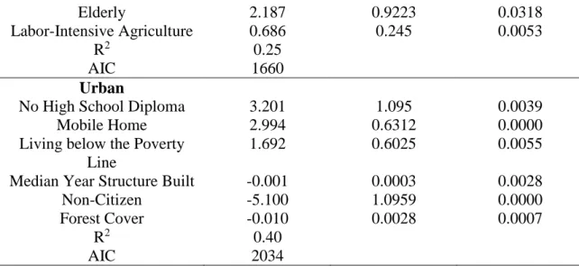
Area-Level Factors Coefficient Standard Error P-Value Rural
Mobile Homes 2.292 0.4701 0.0000
Developed Land -0.030 0.045 0.0000
17
Elderly 2.187 0.9223 0.0318
Labor-Intensive Agriculture 0.686 0.245 0.0053
R2 0.25
AIC 1660
Urban
No High School Diploma 3.201 1.095 0.0039
Mobile Home 2.994 0.6312 0.0000
Living below the Poverty Line
1.692 0.6025 0.0055
Median Year Structure Built -0.001 0.0003 0.0028
Non-Citizen -5.100 1.0959 0.0000
Forest Cover -0.010 0.0028 0.0007
R2 0.40
AIC 2034
Table 2: Ordinary least regression model output for rural and urban location
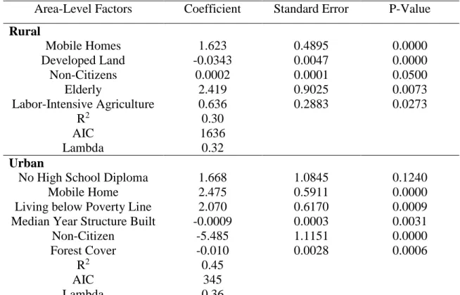
Spatial autocorrelation in the OLS residuals may be the result of autocorrelation of the dependent variable (i.e. spatial lag) or autocorrelation in the error term (i.e. due to spatially autocorrelated predictors that are not included in the model). The Lagrange Multiplier test identifies which form of spatial autocorrelation is present and what model type is best through the calculation of a Robust Lagrange Multiplier Index. Index values for both rural and urban locations indicate that the spatial error regression tends to be more significant (statistically significant: p-value <0.01) than the spatial lag regression model. Hence, the spatial error model is the more appropriate model specification for this data (Anselin 1988).
In the spatial error regression model, the spatial error term incorporates spatial dependence into the error term (Anselin and Bera 1998).
𝑦 = 𝑋𝛽 + 𝜀 with 𝜀 = 𝛾𝑊 + 𝜑
where W is spatial weights matrix, is the vector error terms, 𝜀 are spatially lagged errors, and 𝜑 is a vector of independent random errors. 𝛾 is an autoregressive coefficient, which describes the
18
(Anselin and Bera 1998). In order to apply the methods of spatial regression analysis, we needed to express the nearness of geographic units, using a spatial weights matrix (W) (GeoDa version 1.6.6, Tempe, AZ). The spatial weights matrices were assigned a first-order contiguity weights matrix (e.g. queen contiguity); where we considered ZIP codes that shared boundaries and vertices as contiguous (Anselin and Bera 1998, Aneslin et al. 2006).
Spatial error regression models were constructed for both rural and urban locations, using the same variables that were significant at the 95% confidence level in the OLS models. The results of the spatial error regression models are presented in Table 3. The residuals of both the urban and rural spatial error regression model exhibited no significant spatial autocorrelation. This finding further confirms that the spatial error regression model successfully incorporates the spatial effects.
Area-Level Factors Coefficient Standard Error P-Value Rural
Mobile Homes 1.623 0.4895 0.0000
Developed Land -0.0343 0.0047 0.0000
Non-Citizens 0.0002 0.0001 0.0500
Elderly 2.419 0.9025 0.0073
Labor-Intensive Agriculture 0.636 0.2883 0.0273
R2 0.30
AIC 1636
Lambda 0.32
Urban
No High School Diploma 1.668 1.0845 0.1240
Mobile Home 2.475 0.5911 0.0000
Living below Poverty Line 2.070 0.6170 0.0009
Median Year Structure Built -0.0009 0.0003 0.0031
Non-Citizen -5.485 1.1151 0.0000
Forest Cover -0.010 0.0028 0.0006
R2 0.45
AIC 345
Lambda 0.36
19 Results
Figure 1 shows the incidence rate of heat-related ED visits by ZIP code across North Carolina for the warm season months (May-September) of 2007-2012. The majority of locations with high HRI incidence rates were located in the southern Coastal Plain or the southeastern region of North Carolina. The bottom 10% of ZIP codes with the lowest HRI incidence had less than 3.4 ED visits per 100,000 person-years. These locations were concentrated around
metropolitan cities including, Raleigh, Durham, Greensboro, Charlotte, and Winston-Salem. The top 10% of ZIP codes with the highest HRI incidence had greater than 41.6 ED visits per person-years. These locations were concentrated in rural areas in the southern Coastal Plain of North Carolina, which experiences some of the warmest summer temperatures in North Carolina.
Figure 1: Map of study area featuring major cities and heat-related illness rates per 100,000 person-years. ZIP codes defined as urban using the 150 people per square kilometer definition are highlighted in black. Cities include Charlotte, Greensboro, Raleigh,
20
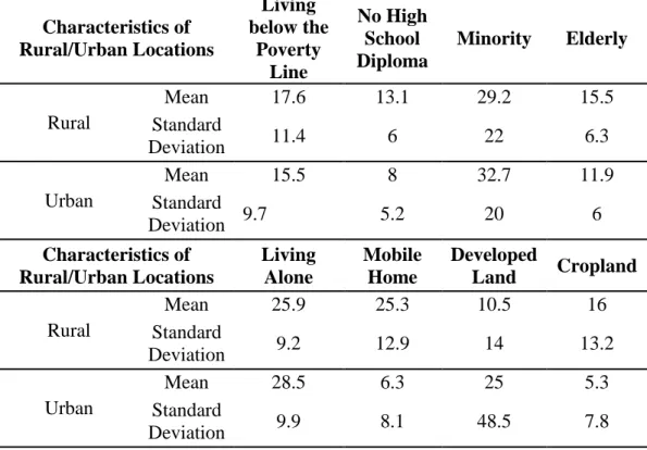
Overall, urban locations had fewer total HRI ED visits (42 .7% of the total HRI ED visits) than rural ZIP locations (57.3% of total HRI ED visits). Accounting for age and gender specific populations, these differences are even further pronounced with 19.7 ED visits per 100,000 person-years in urban locations and 33.5 ED visits per 100,000 person-years in rural locations. Generally, rural locations displayed a greater percentage of cropland, population living below the poverty line, mobile homes, elderly, and residents without a high school diploma
or living alone. Urban locations showed a greater percentage of residents with a race other than white and percent developed land (Table 4).
Characteristics of Rural/Urban Locations Living below the Poverty Line No High School Diploma
Minority Elderly
Rural
Mean 17.6 13.1 29.2 15.5
Standard
Deviation 11.4 6 22 6.3
Urban
Mean 15.5 8 32.7 11.9
Standard
Deviation 9.7 5.2 20 6
Characteristics of Rural/Urban Locations Living Alone Mobile Home Developed
Land Cropland Rural
Mean 25.9 25.3 10.5 16
Standard
Deviation 9.2 12.9 14 13.2
Urban
Mean 28.5 6.3 25 5.3
Standard
Deviation 9.9 8.1 48.5 7.8
Table 4: Mean and Standard Deviation of Area-Level Risk Factors in Rural and Urban Locations
21
non-developed land, and more agricultural labor hours predict higher rates of HRI incidence. Increases in elderly (i.e. age greater than 65 years old) predicted the largest increase in HRI, with 10.23 ED visits per 100,000 person-years. Increases in mobile homes and agricultural labor hours predicted 4.07 and 0.89 ED visits per 100,000 person-years, respectively. Increases in the
percent developed land predicted decreases in ED visits per 100,000 person-years (Table 3).
Although non-citizens were significant in the rural model, it only predicted marginal increases in ED visits.
The urban spatial error regression model explained 45% of variance of HRI ED visits (Table 3). It reveals that urban locations with a greater percent of mobile homes, people with no high school diploma, and people living below the poverty line predict higher rates of HRI incidence. Whereas, urban locations with a greater percent of non-citizens, forested land cover, and newer median year structure built lower rates of HRI. Increases in mobile homes, no high school diploma, and living below the poverty line predicted increases in HRI incidence of 10.9,
4.3, and 6.9 ED visits per 100,000 person-years, respectively. Increases in non-citizens, median year structure built, and forested land cover predicted decreases in HRI incidence of 1.0,
-0.0009, and -0.010 ED visits per 100,000 person-years, respectively.
Discussion
22
incorporated, including the number of mobile homes, non-citizens, and estimates of agricultural labor intensity. Spatial regression models were constructed separately for rural and urban locations, with each explaining 30% and 45% of the variance of HRI ED visits, respectively.
In urban areas, the best predictors of heat-related ED visits included percent of population lacking a high school diploma, living in mobile homes, living below the poverty line, median year structure built, percentage of forest cover, and percentage of non-citizens. Most of these risk factors are consistent with previous heat-health studies, which are focused on urban areas. Specifically, living in poverty and low educational attainment (i.e. no high school education) are well-established risk factors for heat-related mortality across many populations and regions (Kim and Joh 2006; Naughton et al. 2002; O’Neill et al. 2005). In our study, both of these risk factors
predicted large increases in HRI ED visits in the urban locations (i.e. 6.9 and 4.3 ED visits per 100,000 person-years, respectively).
Forest cover and newer buildings have been identified as protective factors against adverse heat-health outcomes in urban environments (Vandentorren et al. 2006). Vegetation mitigates the urban heat island effect by reducing heat exposure, while older buildings often have deteriorating and insufficient insulation, which can affect the efficiency of air conditioning and increase heat exposure. However, our results only demonstrated a marginal decrease in
predicted HRI with respect to these two variables.
23
Specifically, these immigrants are often of Asian descent and fulfill the growing demand for highly-skilled workers to fuel entrepreneurship and continued employment in the technology industry within these urban locations (Appold 2014). In addition, mobile homes predicted a large increase in the number of HRI ED visits within the spatial regression model. Mobile homes are an affordable housing option for low-income households in North Carolina and have not been studied in the context of heat-related morbidity or mortality (Rust 2007). Mobile homes are often energy inefficient, with little or no insulation in the walls, ceiling, floor, or doors (U.S Energy Information Administration 2010). Poor insulation limits the ability of air conditioning units to sufficiently cool the mobile home. This problem is compounded when residents cannot afford to run air conditioning for extended periods of time (Arman and Yarnal 2010).
In rural areas, the greatest risk factors for heat-related ED visits included elderly, labor-intensive agriculture, mobile homes, non-citizens, and developed land. Percent elderly (e.g. population greater than 65 years old) predicted the largest increases in HRI incidence. As noted in multiple heat-health studies, elderly have a biological predisposition towards heat stress causing them to be more sensitive to heat than younger populations (Basu 2009; Chow et al. 2012; Kovats and Hajat 2008; Vandentorren et al. 2006). In comparison to urban locations, rural elderly also tend to be of a lower socioeconomic status, which may further increase their
vulnerability to HRI (Coburn and Bolda 2001). This difference in socioeconomic status may explain why older residents in urban locations do not predict HRI incidence.
24
40% of North Carolina farm workers experience at least one HRI symptom while laboring in extreme heat (Mirabelli et al. 2010). In some cases, HRI cases can lead to death. A review of medical examiner records from 1977 to 2001 across the state identified nearly 50% of all occupational heat-related deaths also occurred within this group. These deaths often arose from physical labor in hot weather (Mirabelli and Richardson 2005). In addition, other research has highlighted that poor housing, lack of access to social networks and health care also make farmworkers particularly vulnerable to heat (Montz et al. 2011, Quandt et al. 2013).
Investigation of the percentage of farm worker populations contributing to ED HRI visits relative to the proportion of labor-intensive agriculture would be an important direction for greater understanding of these patterns.
An additional risk factor for HRI in rural locations is the numbers of non-citizens. In contrast to urban locations, the number of non-citizens corresponded with increases in HRI ED visits in rural areas. While this may be related to the isolation experienced by some non-citzens (Chow et al. 2012; Harlan et al. 2013), many non-citizens in rural North Carolina perform agricultural labor (Carroll et al. 2011) and therefore are highly exposed to the heat and exertion heat stress from physical labor (May 2009).
Similar to urban locations, mobile homes predicted a large increase in heat-related ED visits in rural areas. Many mobile home owners cannot afford high energy bills that occur when attempting to cool poorly insulated mobile homes, particularly during the hot summer months. Harrison and Popke (2010) conducted interviews in rural North Carolina that provide evidence of unaffordable energy bills, some as high as $400 USD during the warmest months of the year.
25
research, which has mostly been carried out in urban locations, where effects of the urban heat island contribute to heat-related mortality or morbidity (Anderson and Bell 2011; Luber and McGeehin 2008). As reported earlier, rural areas in North Carolina experience significantly greater incidence rates of HRI ED visits, and underlying social vulnerabilities (e.g. poverty, low educational attainment) in rural areas are a greater concern for increased HRI.
It is important to discuss some limitations of this study. The counts and rates presented are likely underestimates of the true occurrence of HRI in North Carolina emergency
departments, since data from NC-DETECT does not include ED visits for federally run hospitals (military and Indian Health Services) and other health clinics, such as urgent cares. Secondly, we analyzed data across ZIP code areas, which do not capture socioeconomic and demographic differences as effectively as census boundaries (Krieger et al. 2002). Thirdly, the use of single classes of rural and urban on the basis of population density does not allow for the capture of intervening areas in the urban-rural continuum (e.g. suburban, rural near urban areas etc.). Future analysis should incorporate gradations of urban and rural as well as proximity to urban areas. Lastly, we based our study on area-level measures, evaluating the risk factors at a
population level rather than an individual level. Subsequently, we can only make suggestions of the causal pathways that alter individual health at the ZIP code level. Further research is needed to identify the effects of heat at an individual level.
Conclusion
26
factors for heat morbidity rather than heat mortality. Second, it demonstrates that rural
27
CHAPTER 3: RELATIONSHIPS BETWEEN HRI AND TEMPERATURE
Exposure to extreme heat is the most common cause of weather-related fatalities in the United States (NOAA 2007). This extreme heat exposure is detrimental to a person’s health
when it overwhelms their ability to thermoregulate, increasing the likelihood of succumbing to heat-related illnesses (Luber and McGeehin 2008). Heat-related illnesses (HRI) range from mild heat cramps to heat exhaustion, heat syncope and, in the most severe cases, heat stroke, which has a 50% mortality rate (Grogan and Hopkins 2002). Persons with chronic health conditions (e.g. cardiovascular disease, diabetes, or obesity) are more susceptible to the effects of heat, resulting in further increases in morbidity and mortality (Blum 1998). Understanding heat-related morbidity and mortality is of growing importance as climate change is anticipated to increase temperatures and the magnitude and frequency of extreme heat events.
28
temperatures. Often, residents not acclimated to heat, such as populations in northern cities, are more heat-vulnerable, experiencing higher mortality at lower temperatures (Kalkstein and Davis 1989, Curriero et al. 2003). Variation in the temperature and mortality relationship also varies by race, education level, use of air conditioning, and population density (O’Neill et al. 2003,
Kalkstein and Davis 1989). Overall, there is general agreement among the literature that within urban environments, the elderly, minorities, young, poor, and people with underlying medical conditions are the most vulnerable to heat-related mortality and morbidity (McGeehin and Mirbaelli 2001).
Consistent with the previous discussion on temperature and mortality, a number of studies (e.g. Baccini et al 2008, Kovats et al. 2004, Liang et al. 2008, Lin et al. 2009, Alessandrini et al. 2011) also find a V or J-shaped relationship between temperature and
morbidity. The most common morbidities evaluated in these relationships include cardiovascular
29
heat-related illnesses during such events (Knowlton et al. 2009). These heat-related health outcomes are a considerable burden in terms of reduced quality of life, higher cost of healthcare, and loss of economic productivity (Bambrick et al. 2008).
Unlike the majority of previous research, this study analyzed the association between the daily temperature and heat-related morbidity, rather than heat-related mortality, for six warm seasons (May – September) from 2007 to 2012. These relationships are evaluated across different regions (e.g. coastal plain, piedmont) and demographics (e.g. gender, age) within the state of North Carolina to determine the differential impact of heat stress across populations. In particular, we examine variations across rural populations, which are seldom addressed in the heat-health literature. North Carolina is an optimal location to conduct this research because of its large, diverse, and growing population, humid subtropical climate, topographic variability, and statewide surveillance emergency department network. Ultimately, results from this study will provide a better understanding of how temperature affects human morbidity and vulnerable populations, which is not only crucial to the medical community, but to policy makers and
community leaders who develop mitigation and intervention strategies for extreme temperatures.
Methods
Data sources
30
county of residence, and ZIP code of residence of the patient, as well as the date and time of the ED visit, and up to 11 diagnoses at discharge coded using the 9th revision of the International
Classification of Disease (ICD-9-CM). NC DETECT provided ED visit data for 92% of the population in 2007 and 99% by 2008, allowing for statewide coverage of HRI incidence rates (Rhea et al., 2012). NC DETECT does not include ED data from federally operated military hospitals (Womach Army Hospital at Fort Bragg near Fayetteville and Naval Hospital at Camp Lejune near Jacksonville) or Indian Health Services hospital (Cherokee Indian Hospital) located on the Qualla Boundary. ED visits containing at least one heat-related code (ICD-9-CM code 992.xx) in any of the 11 diagnostic fields were used in this study to calculate the incidence of HRI. This code accounts for the effects of heat and light and includes diagnostic codes such as, heat stroke (992.0), heat syncope (992.1), heat cramps (992.2), heat exhaustion (992.3-992.5), heat fatigue (992.6), heat edema (992.7) and other specified and unspecified heat effects (992.8-992.9). The resulting dataset contains a total of 13, 364 ED visits for HRI covering the warm season months (May-September) from 2007-2012.
Age- and gender- specific estimates of the population included in this analysis were obtained from the United States Bureau of Census. The 2010 Census-based population estimates were used as denominators in the estimation of HRI ED visits per 100,000 person-years. Other socioeconomic, employment, and housing data were collected from the five-year estimates from the American Community Survey for 2008 to 2012 at the ZIP code level. These data were used to characterize ZIP code locations and regions. In order to obtain rates for different
31
Daily maximum temperature observations were obtained from weather stations maintained by the National Weather Service and Federal Aviation Administration, the U.S. Forest Service, as well as stations in the North Carolina Environment and Climate Observing Network. In total, 169 weather stations were used across the following networks: the Automated Surface Observing System (ASOS), the Automated Weather Observing System (AWOS), the Remote Automatic Weather Station network (RAWS), and the North Carolina Environment and Climate Observing Network (EcoNet). The ZIP code of the patient’s residential address was
utilized to determine which weather station to assign to each ED admission. Specifically, the shortest distance was determined between the center of the patient’s ZIP code area and the weather station based on the shortest Euclidean distance using the great circle distance formula:
D = Rcos-1[sinl1 sinl2+cos l1 cosl2cos(m2-m1)]
where D is the distance (km) between the ED admission and the weather stations, R is the mean earth radius, l1 and l2 are the latitudes (rad) of the ED visit and weather station, respectively, and m1 and m2 are the longitudes (rad) of the ED visit and weather station, respectively (Cao, et al.
2004). Each ED visit was assigned a latitude and longitude based on the centroid of the patient’s ZIP code address.
32
hypothesize that there is greater spatial variability in heat index values due to microclimatic variations in humidity (e.g. effects of vegetation, bodies of water). Because the network of weather stations used in this study is too sparse to capture this variability, the relationship between HRI and maximum heat index is not as strong. In contrast, the maximum temperature displays more modest microclimatic variations, thus providing a more spatially robust measure of heat stress. Fahrenheit scale was used for data management and analysis. Celsius
conversions were also presented in consideration of non-United States and scientific readers.
Figure 2: HRI ED visits per 100,000 person-years for maximum temperature and heat index versus heat-related illness.
Urban and rural character
33
spend much of their time inside in an air conditioned environment). The study area was therefore classified into four regions on the basis of the urban-rural character of the landscape and the Census-determined work commuting flows between areas (e.g. rural residents
commuting to urban areas or remaining in rural areas) (Hartz et al. 2005). Regardless of whether a person lives in a rural or urban environment, large portions of their workday are spent at their place of occupation. In the case of HRI, specific occupational environments can promote (e.g. construction, agriculture) or reduce (e.g. office) heat exposure.
Rural-Urban Commuting Area (RUCA) codes were used to differentiate areas according to their economic integration (i.e. commuting patterns) with urban areas or other rural areas (WWAMI Rural Health Research Center 2004). RUCA codes were assigned to each United States ZIP code based on markers of population density, with values ranging from 1.0 (most urban) to 10.6 (most rural). In this study, ZIP codes were classified into one of four mutually exclusive RUCA groups (Table 5): 1) Metropolitan, defined as the most urban containing populations that reside and work in large urban environments; 2) Rural metropolitan, defined by a low population density, low values of impervious surface area, and large portions of its
residents commuting and employed in nearby metropolitan locations; 3) Rural town, including larger towns and adjacent rural areas where few people commute into metropolitan locations; and 4) Rural isolated, the most rural category, including populations that reside in small towns and adjacent rural areas.
Location RUCA code Definition
Metropolitan 1.0 Census defined Urban Areas (e.g. Greater than 50,000 population)
Rural Metropolitan 2.0-3.0, 4.1, 5.1, 7.1, 8.1, 10.1
Locations with substantial commuter flows to Urban Areas (30% to 50%) Rural Town 4.0, 4.2, 5.0, 5.2, 6.0,
6.1
34
commuter flows to Urban Areas (Less than 29%)
Rural Isolated 7.0, 7.2-7.4, 8.0, 8.2-8.4, 9.0-9.2,10.0,10.2-10.6
Census defined (small) Urban Clusters (e.g. 2,500 to 9,999 population) with commuter flows to Urban Clusters (Less than 50%) and
minimal flows to Urban Areas (Less than 29%)
Table 5: Definition of Metropolitan, Rural Metropolitan, Large Rural City, and Rural and Isolated Town from Rural-Urban Commuting Codes (RUCA codes).
Statistical analysis
35
provides a direct estimate of the rate of HRI expected on a day with a given maximum temperature.
Two summary statistics were developed from the GAM models and compared across different populations in the study area.
1) The threshold temperature, which represents the maximum temperature in which a significant elevation in HRI is observed. In studies of heat-related mortality, this defines the inflection point in the “U- or J- shaped” relationships between temperature and mortality. Applying similar methods, we defined the threshold temperature as the temperature in which HRI ED visits were statistically different from zero (at the 95% confidence level) and remain significant for higher temperatures (Davis et al. 2003, Gosling et al. 2014).
2.) Peak temperature, which is the daily maximum temperature in which the greatest rates of HRI ED visits occurred. All statistical analysis was conducted using R software 3.0.1 with the MGCV package (R Core Team 2013, Wood 2006, Wood 2011).
Results
Basic characteristics of HRI across North Carolina
Figure 3 illustrates the incidence rates of HRI ED visits by ZIP code across North
36
(96 ˚F) (Figure 4a). Temperature of this magnitude are quite common across the eastern
two-thirds of the state (e.g. approximately 10% to 15% of days within warm season) during the months of June through August (North Carolina State Climate Office 2014).
Figure 3: HRI ED visits per 100,000 person-years for May through September from 2007 to 2012. HRI ED visits are acquired through NC-DETECT. Map also includes regional locations and cities with metropolitan characteristics.
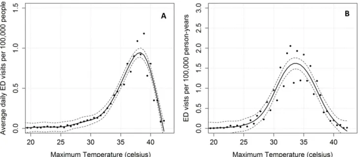
Figure 4b depicts the daily average rates of HRI ED visits across North Carolina with respect to temperature. HRI ED visits increase strongly at the threshold temperature of 30.6 ˚C (87 ˚F) and reach a peak at 38.3˚C (101 ˚F). Above this temperature, there is a very marked
37
Figure 4: HRI versus maximum temperature across North Carolina for May - Sept 2007 to 2012 (a) Daily HRI ED visits per 100, 000 people with respect to maximum temperature; (b) HRI ED visits per 100,000 person-years relative to maximum temperature for North Carolina
Regional characteristics of HRI
HRI ED visits were significantly lower in the Mountains region compared to the Piedmont and Coastal Plain (Table 6). Owing to its higher elevation, most portions of the Mountains region rarely experience maximum temperatures above 35˚C (95 ˚F). Indeed, its threshold temperature of 26.7 ˚C (80˚F) for HRI was the lowest threshold temperature observed
in this study. Additionally, the Mountain region displayed the lowest peak temperature (33.3˚C, 92 ˚F) across the three regions. The populous Piedmont region, on the other hand, experienced
38
Table 6: Regional and demographic characteristics of HRI including the crude incidence rates (i.e. HRI ED visits per 100,000 person-years), the threshold temperatures, peak temperatures, and maximum ED visits with respect to the peak temperature value.
The Coastal Plain exhibited significantly higher rates of HRI ED visits than the Piedmont and Mountains. The peak temperature for ED visits was 37.8˚C (100 ˚F), with significantly more ED visits (1.53 daily HRI ED visits) than the Piedmont (0.62 daily HRI ED visits) and
Mountains (0.35 daily HRI ED visits) for peak temperatures. The threshold temperature was 31.7 ˚C (89 ˚F), which was lower than the Piedmont, suggesting the population’s greater vulnerability
to heat. All three regions exhibited a large decline in HRI ED visits after peak temperatures. This decline is especially precipitous across the Coastal Plain, even though the number of HRI ED visits remained higher than the other two regions (Figure 5). Due to the low incidence of
ED visits per 100,000 person-years (HRI incidence Rates) Threshold Temperature ˚C(˚F) Peak Temperature ˚C(˚F) Daily Maximum ED visits Regional
Mountains 11.6 26.7(80) 33.3(92) 0.35
Piedmont 20.3 31.7(89) 37.8(100) 0.62
Coastal Plain 34.7 31.1(88) 37.8(100) 1.53
Rural and Urban
Metropolitan 18.8 32.2(90) 38.3(101) 0.62
Rural Metropolitan 26.7 32.2(90) 37.2(99) 1.00
Rural Town 37.7 30.6(87) 38.3(101) 1.24
Rural Isolated 38.6 31.7(89) 37.8 (100) 1.86
Age (years)
Under 14 6.2 n/a 37.8(100) 0.19
15 to 17 34.8 31.7(89) 37.8(100) 1.06
18 to 44 35.6 31.1(88) 37.8(100) 1.32
45 to 64 25.8 31.7(89) 38.3(101) 1.01
39
HRI in the mountain region, and a different relationship with HRI at lower maximum temperatures, the remainder of the analysis focused on the Piedmont and Coastal Plain.
Figure 5: Daily HRI ED visits per 100, 000 people with respect to Maximum Temperature for different physiographic regions of North Carolina (i.e. Mountains, Piedmont, and Coastal Plain)
Rural and urban characteristics of HRI
In the assessment of the rural-urban characteristics of HRI, Table 6 reveals that incidence rates of HRI increased with the rurality of the region. Specifically, rural isolated populations displayed significantly higher HRI ED visit rates between temperatures of 31.7 ˚C (89 ˚F) and 40˚C (104 ˚F) compared to the other urban-rural categories. The differences across the four
40
were also lower compared to the more urban locations (i.e. metropolitan and rural metropolitan) (Figure 6).
Figure 6: Daily HRI ED visits per 100,000 people with respect to maximum temperature for different rural-urban regions (i.e. metropolitan, metropolitan rural, rural town, and rural
isolated)
Demographic characteristics of HRI
41
to 17 and 55 to 64 age demographic. The metropolitan-rural differences in HRI rates were most pronounced in the 18 to 34 age demographic.
Figure 7: HRI ED visits per 100, 000 person-years (i.e. HRI incidences) for different age demographics across the rural-urban continuum
Figure 8 illustrates relationships between HRI by age group and maximum temperature. The relationships display generally parallel forms. Threshold temperatures were similar across age groups, but there were marked differences in the rates near the peak temperature, with those in the 18 to 44 age group nearly double HRI rates of the under 14 age group. Peak temperatures across the five groups are remarkably similar, though the peak for the 45 to 64 age group is slightly higher (38.3 ˚C, 101 ˚F) and the 15-17 age group slightly lower (37.2˚F, 99 ˚F). Due to
42
Figure 8: Daily HRI ED visits per 100, 000 people with respect to maximum temperature for different demographics
43
Age (years) Female Male
Under 4 2.5 2.7 5 to 9 3.1 5.6 10 to 14 12.8 16.9 15 to 17 23.3 45.8 18 to 24 16.6 49.7 25 to 34 13.5 55.9 35 to 44 12.9 47.8 45 to 54 13.5 45.0 55 to 64 23.5 55.2 65 to 74 13.0 34.7 75 to 84 16.6 36.3 85 and older 25.8 39.2
Table 7: Demographic characteristics of HRI incidence rates for males and females (incidence rates are reported as 100,000 person-years).
Discussion
This study investigated the association between the maximum temperature and heat-related morbidity in North Carolina across six warm seasons (e.g. May to September) from 2007 to 2012. The impact of temperature on human health has been studied extensively, however, most epidemiological studies have focused on the relationship between temperature and
mortality in urban locations. Unlike previous studies, this study examined the relationship with heat morbidity rather than heat mortality. In addition, this relationship was investigated across an entire state, allowing for an examination of the differences between rural and urban
44
Previous research reveals a U-or J-shaped curve with mortality peaks at the highest and lowest ends of the temperature spectrum. This study focused on the warm season and
consequently, the higher end of the temperature spectrum. At the state level, results from this study indicated that the temperature and morbidity curves also followed a J-shape curve with HRI visits beginning to increase at a threshold temperature of 30.6˚C (87 ˚F). However, in our study the J-shape curve reached a maximum at 38.3˚C (101 ˚F), with the highest HRI rates occurring at this temperature. At extremely high temperatures (temperatures higher than 38.3˚C) HRI rates declined considerably. To our knowledge, this type of decline has not been reported in the research. Hartz (2013), for example, observed increased rates of heat-related 9-1-1
emergency dispatches at maximum temperatures above 38.3˚C (101 ˚F) in Chicago, Illinois,
USA and Phoenix, Arizona USA. Also, Curriero et al. (2003) has observed linear or exponential increases in heat mortality at higher temperatures in other cities across the United States.
Noteworthy exceptions to the J-shape curve can be found when evaluating specific health outcomes. For instance, Xiang et al. (2014), evaluated associations between maximum
temperature and work-related injuries and found a positive association with temperatures below 100 ˚F and a decline when temperatures exceeded this peak temperature. Xiang et al. (2014)
45
allowing many residents to stay indoors and prevent HRI with air conditioning use. Additional coping mechanisms include a North Carolina High School Athletic Association mandate to suspend athletic practice at high temperatures and other recommendations by the North Carolina Department of Labor to mitigate occupational risk during extreme heat (North Carolina
Department of Labor 2011, North Carolina High School Athletic Association 2014). Future HRI mitigation strategies should emphasize adaptive and coping measures at lower temperatures (i.e. 35 to 37.8 ˚C, 95 to 100 ˚F) to prevent HRI ED visits.
Regionally, the Mountains experienced significantly lower HRI ED visit rates than the Piedmont and Coastal Plain. The higher elevations (305 -2098 meters) of this region experience relatively cooler temperatures throughout the summer. The threshold temperature for the
Mountain region (26.7˚C, 80˚F) was also lower than other regions, suggesting that its population
is less acclimatized to heat. This result is consistent with Curriero et al. (2003) and Kalkstein and Davis (1987), who found regional differences in acclimatization, with cooler northern cities experiencing higher rates of heat mortality than southern cities.
The Coastal Plain displayed a lower temperature threshold (i.e. 31.1˚C, 88 ˚F) and greater
46
symptom while laboring in extreme heat from June through September in 2009. Many of these workers are migrant and seasonal farm laborers, and the greatest concentration of these workers reside in the Coastal Plain counties of Duplin, Sampson, and Wayne County (Montz et al. 2011). Migrant and seasonal farm laborers, are particularly heat vulnerable, as they not only experience HRI through strenuous activity in high temperatures, but also from dangerous hot indoor
conditions within housing structures (Quandt et al. 2013).
To investigate the relationship between temperature and HRI across different regions within the urban-rural continuum of the study area, ZIP codes were categorized as Metropolitan, Rural Metropolitan, Rural Town, and Rural Isolated based on their population density and work commuting patterns. To date, few studies have examined the effect of temperature on rural populations. The lack of research likely relates to the well-established understanding among researchers that an urban environment is an important risk factor for heat-related morbidity and mortality, mainly due to the urban heat island effect (McGeehin and Mirabelli 2001). In North Carolina, however, we found that rural populations displayed significantly higher rates of HRI than the urban populations. Moreover, our results established that rates of HRI ED visits are greatest in isolated rural areas and rural towns relative to rural areas situated near larger cities, where many people commute to the city.
The Isolated and Rural locations experienced nearly a threefold increase in HRI at 37.8˚C (100 ˚F) compared to more urban regions. Additionally, rural locations (e.g. Rural Town and Isolated Rural) displayed a lower threshold temperature (e.g., 30.6 to 31.7 ˚C, 87 to 89 ˚F),
compared to urban populations (32.2 ˚C, 90 ˚F). Several factors likely contribute to the heat vulnerability of rural residents. These factors may relate to the population’s underlying social
47
factors affect their capacity to cope with heat. One common factor that increases social vulnerability is poverty, a well-established risk factor for both heat morbidity and mortality (Anderson and Bell 2011). In the urban-rural continuum of regions, poverty levels increased from 15.2% (Metropolitan) to 20.1% (Rural Isolated), coincident with increasing rates of HRI. Other risk factors that influence social vulnerability include the proportion of the population with low educational attainment (i.e. no high school education) and older building structures (i.e. more energy inefficient) were also greater in rural locations (Table 8).
RUCA classification Percent Mobile Homes Percent of residents living below the poverty line Percent of residents with no high school
education
Population Density
Metropolitan 8 15.2 12.8 465
Metropolitan
Rural 26 16 18.1 60
Rural Town 23 17.6 18.5 94
Rural Isolated 25 20.1 20.3 35
RUCA classification Median Year Structure Built Percent Cropland Percent Developed Land
Percent of residents within the farming, fishing, and forestry
occupation
Metropolitan 1982 9.9 43.7 0.096
Metropolitan
Rural 1985 12.7 8.8 0.582
Rural Town 1979 19.4 13.5 0.583
Rural Isolated 1978 19.1 7.8 1.305
Table 8: Socioeconomic, housing, and land cover characteristics of rural and urban locations. Percent were calculated from a total population across each rural-urban ZIP code region (e.g. percent mobiles homes of total households).
48
however, is more likely to engage in outdoor exertional activities associated with their occupation. In fact, these rural regions contain significantly more cropland and a greater proportion of the population engaging in agriculture (Table 8). As was observed in the Coastal Plain, farm laborers who engage in agriculture are predisposed to HRI due to outdoor exposure and strenuous labor. This occupational risk and added social vulnerability are a plausible explanation for the exceptional rates of HRI. Future research should explore patterns of HRI at the individual-level to understand the specific pathways (e.g. occupation, social vulnerability, etc.) that result in high HRI in rural communities.
Overall incidence rates of HRI were highest among the 15 to 64 age demographic, particularly the 18 to 44 age group. These results contradict previous research, which focused on excess morbidity and mortality during heat waves and found that the elderly, very young, and the debilitated (i.e. underlying medical conditions) were more likely to experience heat-health effects (e.g. Knowlton et al. 2009). In contrast, we found that these populations (i.e. young, elderly) experience significantly lower rates of HRI across North Carolina, even at the highest temperatures, which are typically experienced during heat wave events.
The average rates of HRI ED visits for males were three times greater than that for