DENSE GRAPH LIMITS AND APPLICATIONS
Suman Chakraborty
A dissertation submitted to the faculty of the University of North Carolina at
Chapel Hill in partial fulfillment of the requirements for the degree of Doctor of
Philosophy in the Department of Statistics and Operations Research.
Chapel Hill
2018
ABSTRACT
SUMAN CHAKRABORTY: Dense Graph Limits and Applications
(Under the direction of Shankar Bhamidi and Andrew Nobel)
In recent years, there has been a growing need to understand large networks and to devise
effective strategies to analyze them. In this dissertation, our main objectives are to understand
various structural properties of large networks under suitable general framework and develop general
techniques to analyze important network models arising from applied fields of study.
In the first part of this dissertation, we investigate properties of large networks that satisfy
certain local conditions. In particular, we show that if the number of neighbors of each vertex
and co-neighbors of each pair of vertices satisfies certain conditions then the number of copies of
moderately large subgraphs is approximately same as that of an Erd˝
os-R´
enyi random graph with
appropriate edge density. We apply our results to different graph ensembles including exponential
random graph models (ERGMs), thresholded graphs from high-dimensional correlation networks,
Erd˝
os-R´
enyi random graphs conditioned on large cliques and random d-regular graphs.
In the second part of this dissertation, we study models of weighted exponential random graphs
in the large network limit. These models have recently been proposed to model weighted network
data arising from a host of applications including socio-econometric data such as migration flows
and neuroscience. We derive limiting results for the structure of these models as the number of
nodes goes to infinity. We also derive sufficient conditions for continuity of functionals in the
specification of the model including conditions on nodal covariates.
ACKNOWLEDGEMENTS
Firstly, I would like to thank Thami, Maa, and Didi for their unconditional support in all the
endeavors that I undertook throughout my life. It is not possible to describe all the sacrifices that
you have made for bringing me up as whatever I am today. I know, you have never expected
anything from me, but I hope that I have made you proud and happy with this small academic
achievement. I feel lucky that I belong to such a caring family. I have missed you, and I apologize
for being so far, and for so long. Didi, you are my closest companion, and I owe you an answer at
this point. Let me quote The Beatles, and you would understand. “What did you see when you
were there? Nothing that doesn’t show.”
It goes without saying that I could not have written this dissertation without the support
and encouragement of my advisors Shankar Bhamidi and Andrew Nobel. Thank you, Shankar for
keeping my curiosity alive with wonderful problems, and novel ideas. Andrew, thank you for the
time that you spent teaching me how to organize and write scientific ideas in a coherent manner.
Thanks to both of you for your time and patience in answering my questions, suggesting valuable
references, and most importantly showing me the joy of solving problems. I hope to continue
learning more from you in future.
and Bruce Desmarais. I would like to thank Michael Krivelevich for his valuable suggestions on the
content of Chapter 4. I thank Remco van der Hofstad for all the helpful discussions. The outcome
of these discussions are briefly mentioned in the final chapter. Lastly, thank you, Kelly, for being
an awesome collaborator and for all the conversations we had about statistics and life.
Let me thank Alison, Christine, and Samantha for helping me out in a number of situations.
They always had a solution whatever the problem be.
I must thank my fellow Ph.D. students, without them I could not have been able to navigate
this experience. Thank you Debraj for your friendship and all the conversations that we had. Hyo
Young, I do not have any idea how I could have completed my first two years at Chapel-hill without
your support. Thank you so much for that. Raka, thank you for sharing your experiences and for
being an willing ear. Thanks to Eric, Dylan and all others in the department for being part of this
journey.
I will miss our musical band “Phir Kaahe?” and especially the band members when I will
be out of Chapel-hill. Arkopal, Sayan, Sohini, Sujatro, I can not specifically write down your
contributions, but I treasure the time we spent together. Thanks all of you for your friendship.
I want to thank three of my friends who were with me through the most difficult time of my life.
Arghya, Gopinath, and Tanmoy, we are friends for more than two decades, and you guys were sure
of my abilities even when I was not. Thank you for always being there and your encouragement.
Nibedita, I am indebted to you for your support and encouragement throughout my Ph.D. I
must thank you for proofreading parts of this dissertation.
Let me thank Anze and Abhisek (APM) for being awesome friends. Our conversations that
spanned from politics to neuroscience have definitely saved the world. My dissertation is a written
proof of that fact!
Let me thank my friends Aniket, Anwesha, Gol, Sapna, Gargi, Moumita,
Anandita, Cynthia, Anwesha (Florida). Also, thank you Sayan (SDG), Jyotishka (JD), Shalini for
being awesome seniors. I apologize if I have missed someone.
TABLE OF CONTENTS
LIST OF FIGURES . . . ix
1
Introduction . . . .
1
1.1
Why Study Large Graphs? . . . .
1
1.2
Basic Definitions and Notations . . . .
3
1.3
Jumbled Graph by Thomason . . . .
5
1.3.1
Quasi-random Graphs . . . .
5
1.3.2
Szemer´
edi’s regularity lemma and quasi-randomness . . . .
7
1.3.3
Can We do Better? . . . .
9
1.4
Applications . . . 11
1.4.1
Paley Graph . . . 11
1.4.2
Exponential Random Graph Models . . . 12
1.4.3
Random Geometric Graph . . . 12
1.4.4
The Large Clique Problem . . . 14
1.5
From quasi-random graphs to graph limits . . . 15
1.6
Generalized Exponential Random Graph Models . . . 18
1.7
Site Percolation on pseudo random graphs . . . 20
2
Large subgraphs in pseudo-random graphs . . . 23
2.1
Applications of Theorem 2.0.1 . . . 28
2.1.1
Exponential random graph models (
ergm
). . . 28
2.1.2
Thresholded graphs from high-dimensional correlation networks . . . 30
2.1.4
Random
d-regular graphs . . . 33
2.1.5
Optimality of Theorem 2.0.1: Binary graph . . . 35
2.2
Discussion and related results . . . 36
2.2.1
Jumbled graphs . . . 36
2.2.2
Alon’s (n, d, λ) graphs . . . 38
2.2.3
Optimality, limitations and future directions . . . 39
2.3
Notation and Proof Outline . . . 39
2.4
Proof of Proposition 2.3.1 . . . 44
2.5
Preparatory Technical Lemmas . . . 50
2.6
Proofs of Theorem 2.0.1 and Theorem 2.0.4 . . . 64
2.7
Proofs of the applications of Theorem 2.0.1 . . . 72
2.7.1
Proof of Theorem 2.1.2 . . . 72
2.7.1.1
Proofs of Lemma 2.7.3 and Lemma 2.7.4 . . . 74
2.7.2
Proof of Theorem 2.1.5 . . . 78
2.7.2.1
Proof of
(2.7.16)
-
(2.7.17)
.
. . . 81
2.7.2.2
Proof of
(2.7.18)
.
. . . 82
2.7.3
Proof of Theorem 2.1.7. . . 86
2.7.4
Proof of Theorem 2.1.14 . . . 91
3
Generalized exponential random graph Model . . . 96
3.1
Graph limits and Large deviation preliminaries . . . 96
3.2
Generalized exponential random graph Model . . . 98
3.2.1
Model Formulation and Main Theorem . . . 98
3.3
Graph Homomorphisms and scope of GERGM . . . 107
3.4
Discussion . . . 111
3.4.1
Related work: . . . 111
3.5
Proofs . . . 114
3.5.1
Proof of Theorem 3.2.2: . . . 115
3.5.2
Proof of Theorem 3.2.4 . . . 121
3.5.3
Proof of Theorem 3.2.7: . . . 122
3.5.4
Proof of Theorem 3.2.9 . . . 123
3.5.5
Proof of Theorem 3.2.11: . . . 125
3.5.6
Proof of Theorem 3.2.12: . . . 126
3.5.7
Proof of Theorem 3.2.13: . . . 127
3.5.8
Proof of Theorem 3.2.15: . . . 129
3.5.9
Proof of Theorem 3.3.4: . . . 132
4
Site percolation on non-regular pseudo-random graphs. . . 134
4.1
Proof sketch . . . 136
4.2
Notations and Preparatory Lemmas . . . 137
4.2.1
Depth First Search Algorithm(DFS) . . . 137
4.2.2
Technical Lemmas . . . 138
4.3
Proofs of main Theorems . . . 143
4.3.1
Proof of Theorem 4.0.1 . . . 143
4.3.2
Proof of uniqueness under hereditary degree assumption . . . 144
4.3.3
Proving uniqueness under
A1
,
A2
,
A3
. . . 145
5
Discussions and future directions . . . 147
5.1
Multitype Critical Inhomogeneous Random Graphs . . . 148
5.2
Critical behavior of percolation on a converging dense graph sequence . . . 149
5.3
Consistent Estimation in GERGM . . . 152
LIST OF FIGURES
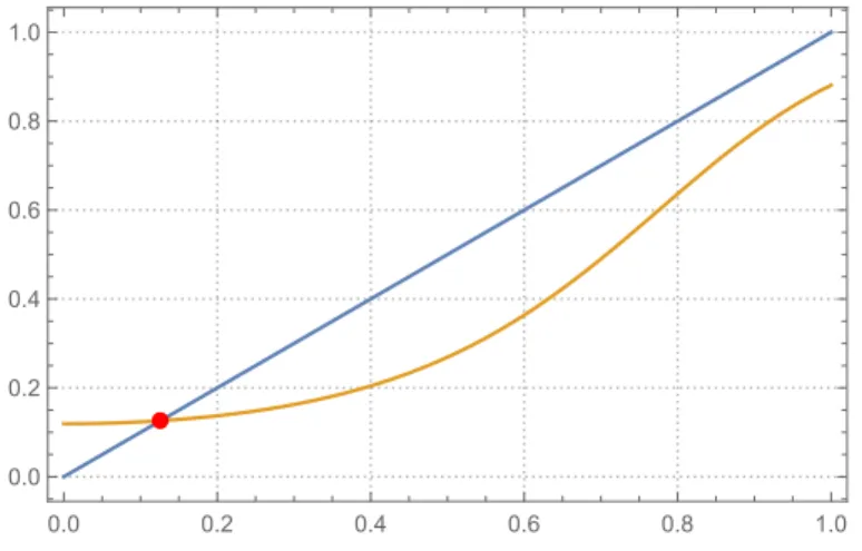
2.1
The functions
f
(p) =
p
and
g(p) =
eβ+γp 21+eβ+γp2
with
β
=
−2 and
γ
= 4.
The red point corresponds to
p
∗. . . 30
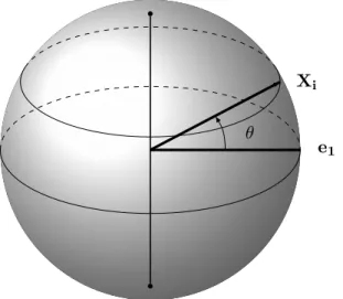
2.2
A vertex
i
is connected 1 in
G(n, d, p) if and only if cos(θ)
>
t
p,d. Here
we have rotated the original points via an orthogonal transformation so
that the co-ordinates of vertex 1 correspond to
e
1= (1,
0, . . . ,
0).
Pic-ture modified from template on
https://github.com/MartinThoma/
CHAPTER 1
Introduction
1.1
Why Study Large Graphs?
Informally, graph theory is the study of pairwise relation between a number of actors.
For example, the actors can be students in a class, brain regions, train stations etc.
and
usually the goal is to understand the pairwise connectivity between these actors. Graph theory
has been a source of beautiful and often intriguing problems. The evolution of the theory
motivated a number of interesting developments in different branches of mathematics, such as
number theory, combinatorics, functional analysis to name a few. A graph is sometimes called
a ‘network’ and we will use both of these names in this thesis. Apart from being a source of
beautiful mathematical theory, it has been turned out to be extremely useful tool for many
applied fields of study. For example, it has found numerous application in computer science,
cryptography, statistical physics, social sciences, biological sciences, statistics and the list goes
on. Next we provide few specific examples to illustrate the ubiquity of large networks.
•
With the rapid growth of internet many huge networks, like Facebook and many others
have emerged in the last decade and one of the pressing need is to understand the nature
and evolution of these networks. The huge size of these networks is one of the main
challenge to analyze them and thus require rigorous understanding of such seemingly
difficult objects.
•
Statistical physics is another important source of intriguing problems in graph theory.
Roughly, it studies interaction between a large number of particles and often the system
of particles are represented by a graph. Often simple looking problems in this area turned
out to be challenging and gave rise to new mathematical techniques. Spin glass, Potts
model are contemporary examples of that.
•
Another example is the telecommunication network. These networks often have an
un-derlying topological structure, for example, in a server network, if two servers are within
certain distance from each other then they are connected. Finding the critical distance
such that no large scale communication breakdown happens is also an area of active
research and known as percolation.
•
Graph theory has also found numerous applications in cryptography. One important
problem is to find the largest set of nodes that are inter-connected (also known as clique).
The difficulty lies in devising an efficient strategy to do this or proving lack of existence of
any efficient strategy. Numerous studies have been done in these area and still a number
of problems remain unsolved.
The examples demonstrate the growing need of understanding large networks and devising
effective strategies to analyze them. Many successful attempts have been made to understand
large networks mathematically and numerous probabilistic and statistical models were proposed
to analyze properties of graphs in general. The literature is enormous to give a comprehensive
review, we will instead focus on some specific aspects of this huge research area. Roughly,
following are the two main objectives of this thesis.
•
Understand various “structural” properties of large networks under suitable general
frame-work.
•
Use the general techniques to analyze important network ensembles arising from applied
fields of study.
triangles (number of three-tuples of actors that are connected to each other) are typical
exam-ples of the former. It is natural to ask the importance of analyzing such structures. It is now
known from various works of last few decades that these structures characterize a network in
a rather strong way and in fact these provide a well defined notion of mathematical limit of
graphs when number of actors are growing to infinity. In the subsequent sections, we make
these statements precise and give an overview of the existing literature. In this regard, we also
discuss some new results and postpone the details to subsequent chapters.
1.2
Basic Definitions and Notations
Let us now formally define a graph and discuss some basic notions.
Definition 1.2.1.
A graph is an ordered pair
G
= (V, E), where
V
is a set of vertices or nodes
and
E
is the set of edges.
Remark 1.2.2.
E
is generally a set of two-element subsets of
V
. For example, if
v
1, v
2∈
V
and
v
1is connected to
v
2then (v
1, v
2)
∈
E. If (v
1, v
2) and (v
2, v
1) are considered different then
the graph is called a directed graph otherwise it is called an undirected graph.
Informally one basic and fundamental line of questions in Graph theory are existence of
graphs with some given properties. Introduction of random graphs helped to produce elegant
solutions to many of them but quite a few of them are still unsolved.
properties of
G(n, p) (see (Bollob´
as, 1998; Janson et al., 2011) and the references therein) in
particular in the large network
n
→ ∞
limit.
One key property of an
Erd˝
os-R´
enyi random graph
is the following: For any two subsets
of vertices
U, W
⊂
[n] the number of edges in a
G(n, p), whose one end point is in
U
and the
other is in
W
, is roughly equal to
p|U
||W
|, where
| · |
denotes the cardinality of a set. Hence,
if a deterministic graph
G
nis similar to
G(n, p), one expects it to satisfy similar properties.
This motivated researchers to consider graphs which possess the above property. The basic
questions are as follows; how to determine when a deterministic graph is similar to a random
graph? How to generate deterministic graphs that are similar to random graph?
Informally, a graph on
n
vertices with similar edge distribution as
G(n, p) is called
pseudo-random graphs. This concept was studied by many authors since mid-eighties and thus acquired
various nomenclature. We will generally use the name pseudo-random graph following
(Kriv-elevich and Sudakov, 2006a). Before delving deep into formal definitions of pseudo randomness,
let us start with a simple property of
G(n, p). For
X, Y
⊂
V
, let
e
G(X, Y
) denote the number
of edges with one end node in
X
and another in
Y
; edges with both end nodes in
X
∩
Y
are
counted twice.
Theorem 1.2.3.
Let
p
=
p(n)
6
0.99. Then for every two (not necessarily disjoint) subsets of
vertices
U, W
⊂
V
the number
e
G(U, W
)
of edges of
G
with one endpoint in
U
and the other
one in
W
satisfies:
|e
G(U, W
)
−
p|U
||W
||
=
O(
√
uwnp).
(1.2.1)
1.3
Jumbled Graph by Thomason
The term “Jumbled” was coined by Thomason in his paper (Thomason, 1987b) to mean
the edges are evenly distributed throughout the graph.
Definition 1.3.1.
A graph
G
= (V, E)
is called
(p, α)-jumbled if
p,
α
are real numbers satisfying
0
< p <
1
6
α
if every subset of vertices
U
⊂
V
satisfies:
e
G(U
)
−
p
|U
|
2
6
α|U
|.
(1.3.1)
In the definition, one can interpret
p
as the edge density and
α
can be interpreted as the
deviation from the true distribution. Indeed, the motivation of such definition can be attributed
to (1.2.1). Note that
G(n, p) is (p, O(
√
np)) jumbled following (1.2.1).
Some simple but interesting consequences of that were proved in (Thomason, 1987b) in the
context of jumbled graphs are for example if a graph
G
is (p, α) jumbled then the complement
graph ¯
G
is (1
−
p, α) jumbled. Also if
G
is (p, α) jumbled then every induced subgraph is also
(p, α) jumbled etc. Notice the smaller the value of
α
more informative the condition (1.3.1)
becomes. After Thomason, one of the cornerstone work was done by Chung, Graham and
Wilson (Chung et al., 1989) in the late eighties.
1.3.1
Quasi-random Graphs
In their remarkable paper (Chung et al., 1989), Chung, Graham and Wilson established
that many “random-like” properties of a large graphs are equivalent. Therefore, one may take
any of these equivalent notions to be a measure of randomness. Chung, Graham and Wilson
(Chung et al., 1989) called a graph quasi-random if it satisfies any of these properties. Before
stating their main result we introduce few notations. Here we work on a sequence of graph
G
n= (V
n, E
n) and for simplicity from now on assume that
V
:= [n] :=
{1, . . . , n}
and for
Denote
λ
1, λ
2, . . . , λ
nas the eigen-values of the adjacency matrix of the
G
narranged
ac-cording to
|λ
1|
>
|λ
2|
> . . . >
|λ
n|. Now we state the main theorem from (Chung et al.,
1989).
Theorem 1.3.2
((Chung et al., 1989))
.
Let
p
∈
(0,
1)
be fixed. Then for any graph sequence
G
n, the following are equivalent:
P
1(r): For any graph
H
on
r
vertices, where
r
>
4
is any arbitrary fixed positive integer
n
∗Gn(H) = (1 +
o(1))n
rp
1
−
p
|e(H)|(1
−
p)(
r2)
,
where
n
∗Gn
(H)
denotes the number of labelled occurrences of the subgraph
H
in
G
n.
P
2(r): Let
C
rdenote the cycle of length r. Let
r
>
4
be even,
e(G
n) =
n
2p
+
o(n
2)
and
n
Gn(C
r)
6
(np)
r
+
o(n
r).
P
3:
e(G
n)
>
n
2p
+
o(n
2)
and
λ
1= (1 +
o(1))np,
λ
2=
o(n).
P
4: For each subset of vertices
U
⊂
[n]
e(U
) =
p
2
|U
|
2
+
o(n
2).
P
5: For each subset
U
n⊂
V
nwith
|U
n|
=
n2
, we have
e(U
n) = (
p8+
o(1))n
2.
P
6: Let
s(v, v
0)
be the number of vertices of
G
njoined to
v
and
v
0the same way: either to
both or to none. Then,
n
X
v6=v0=1
s(v, v
0)
−
(p
2+ (1
−
p)
2)n
=
o(n
3).
P
7:
n
X
v6=v0=1
Remark 1.3.3.
The theorem was proved for
p
=
12but their method can be adapted to extend
the results for any
p
∈
(0,
1). Also notice the condition
P
4implies
G
nis a (p, o(n)) jumbled
graph from (1.2.1). Chung, Graham and Wilson called a graph satisfying any of the seven
equivalent conditions a quasi-random graph. Notice that conditions such as
P
2or
P
7takes
polynomial time to verify but quite strikingly gives control over exponentially many sets such
as
P
4. Another immediate question is “Can we obtain similar results in case of sparse graphs?”
The notion of quasi-randomness is even more difficult when the graph is sparse (p
is allowed to
go to zero as
n
goes to infinity). To the best of our knowledge, the notion of sparse quasi-random
graph was first studied in (Chung and Graham, 2002). They showed that in order to obtain
quasi-randomness one needs additional restrictions on the graph sequence. We will discuss this
notion briefly towards the end of this chapter. We turn our attention again to dense sequence
of graphs and in the next section we introduce an important result by Endre Szemer´
edi. It
is known as Szemer´
edi’s regularity lemma and it is a central tool in the study of dense graph
limits.
1.3.2
Szemer´
edi’s regularity lemma and quasi-randomness
Szemer´
edi’s regularity lemma is a striking result in the context of asymptotic structure of a
graph. Roughly, it tells us that one can partition a large graph into bipartite graphs and each
of these parts looks like a random graph. This beautiful lemma has found applications in many
different branches of mathematics, including number theory, combinatorics and analysis. See
(Koml´
os et al., 2002), for a discussion and applications in graph theory and (Lov´
asz and Szegedy,
2007) for application in analysis. We describe the lemma before discussing its connection to
quasi-randomness.
Let
G
= (V, E) be a simple graph, and let
X, Y
⊂
V
. Then define,
r
G(X, Y
) :=
e
G(X, Y
)
the density of the pair (X, Y
). Given some
δ >
0, call a pair (A, B) of disjoint sets
A, B
⊂
V
δ-regular if all
X
⊂
A
and
Y
⊂
B
with
|X|
>
δ|A|
and
|Y
|
>
δ|B
|
satisfy
|r
G(X, Y
)
−
r
G(A, B)|
6
δ.
A partition
{V
0, . . . , V
K}
of
V
is called an
δ-regular partition of
G
if it satisfies the following
three conditions:
1.
|V
0|
6
δn;
2.
|V
1|
=
|V
2|
=
· · ·
=
|V
K|;
3. all but at most
δK
2of the pairs (V
i, V
j) with 1
6
i
6
j
6
K
are
δ-regular.
Following is the Szemer´
edi’s regularity lemma.
Theorem 1.3.4
((Szemer´
edi, 1978))
.
Given
δ >
0
and an integer
m
>
1
there exists an
integer
M
=
M
(δ, m)
such that every graph of order at least
M
admits an
δ-regular partition
{V
0, . . . , V
K}
for some
K
in the range
m
6
K
6
M.
In their paper (Simonovits and S´
os, 1991), Simonovits and S´
os established a beautiful
relation between quasi randomness and Szemer´
edi’s regularity lemma. Informally it tells that a
quasi random graph admits a
δ-regular partition similar to
G(n, p). Before providing a precise
statement we introduce the following condition.
P
s: For every
δ >
0 and an integer
m
>
1 there exists two integers
M(δ, m) and
N
0(δ, m),
such that such that a graph
G
nwith
n > N
0admits partition
{V
0, . . . , V
K}
for some
K
in the range
m
6
K
6
M
that satisfy
1.
|V
0|
6
δn;
2.
|V
1|
=
|V
2|
=
· · ·
=
|V
K|;
3. all but at most
δK
2of the pairs (V
i, V
j) with 1
6
i
6
j
6
K
satisfy the inequality
|r
G(V
i, V
j)
−
p|
6
δ.
Theorem 1.3.5
((Simonovits and S´
os, 1991))
.
P
sis equivalent to
P
1−
P
7in Theorem 1.3.2.
Thus, Theorem 1.3.5 not only relates quasi random graphs to Szemer´
edi’s regularity lemma
but also provides an equivalent condition for quasi-randomness. Many further properties have
been shown to be equivalent to quasi randomness and we refer the reader to (Graham, 1992;
Simonovits and S´
os, 1997, 2003; Shapira, 2008; Shapira and Yuster, 2010, 2012; Janson, 2011;
Huang and Lee, 2012) for many such properties. We turn our attention to Theorem 1.3.2
again. In particular we focus on the equivalence between
P
1and
P
7.
P
1tells that the number
of induced subgraph of fixed size is asymptotically comparable to that in a random graph.
P
7is
a more local condition and it gives the average co-degree is approximately same as in a random
graphs. A natural question is the following: can we estimate number of copies of a subgraph
whose size is growing with
n? More generally can we control the number of large motifs in a
graph by controlling local structures? In this regard, we report the existing results and our
findings in the next section.
1.3.3
Can We do Better?
Note that condition
P
1ensures the labelled occurrence of a subgraph of fixed size matches
with that of expected number of copies in
Erd˝
os-R´
enyi random graph
with edge connection
probability
p. Our quest begins here. Can we do better than this? For example is it possible
to prove similar result when size of
H
depends and possibly growing with
n? In the context
of quasi-random graphs attempts have been made to prove that
P
1holds even one allows
r
to
go to infinity. In (Chung and Graham, 1990) Chung and Graham showed that if a subgraph
H
sis not an induced subgraph of
G
nthen one must have a set
S
of size
n/2 such that
e(S)
deviates from
n162by at least 2
−2(s2+27)n2. This implies that in a quasi-random graph
G
nat
least one induced copy of every subgraph of size
O(
√
log
n) must be present. The methods of
(Chung et al., 1989) can be adapted to estimate the number of copies of subgraphs of size up
to
O(
√
log
n). Unfortunately, despite our best effort we could not prove or disprove if this can
be improved further without further assumptions.
quasi random graphs we will call them pseudo-random graphs. More precisely, we will assume
that our graph
G
nsatisfies the following two assumptions for some absolute constant
C, and
p, δ
∈
(0,
1):
Assumption A1.
max
v∈[n]
||
Nv
| −
np|
< Cn
δ
.
Assumption A2.
max
v6=v0∈[n]
|
Nv
∩
Nv
0| −
np
2< Cn
δ.
These two conditions are very natural to assume. For example, using Hoeffding’s ineqaulity
it is easy to check that for
G(n, p) assumptions
(A1)
and
(A2)
are satisfied for any
δ >
1/2 with super-polynomially high probability.
As we will see below, besides
G(n, p) there
are many examples of graph ensembles which satisfy assumptions
(A1)
-
(A2)
. Further, these
two specifications are quite basic and often very easy to check for a given graph (random or
deterministic). Under this two assumptions we have been able to improve the results in (Chung
et al., 1989; Chung and Graham, 1990). Informally, our result gives,
If a sequence of graph
G
nsatisfies
A1
and
A2
with parameters (p, δ), then the
number of copies of a subgraph
H
is approximately equal to with that of expected
number of copies of
H
in Erd˝
os-R´
enyi graph with edge connection probability
p
as long as
H
is of size less than or equal to min
12,
(1
−
δ)
loglogγnp
, where
γ
p:=
max{p
−1,
(1
−
p)
−1}.
Of course the statement above is not formal but we make no attempt to make it rigorous in
this chapter, the formal statement is deferred to Chapter 2 but we can observe some clear
improvements over (Chung et al., 1989; Chung and Graham, 1990). We can control the sizes
of subgraphs of size up to
O(log
n) and we precise size threshold up to which we can control
the number of subgraphs. Now we stumble upon the obvious natural question: is it possible
to have control over subgraphs of bigger size? In Chapter 2 we will demonstrate that under
assumptions
A1
and
A2
the obtained results are optimal!
n
vertices whose second largest absolute eigenvalue is
λ. A number of properties of such graphs
have been studied (see (Krivelevich and Sudakov, 2006a) and the references therein). For such
graphs the number of induced isomorphic copies of large subgraphs is also well understood (see
(Krivelevich and Sudakov, 2006a, Section 4.4)). From (Krivelevich and Sudakov, 2006a,
Theo-rem 4.1) it follows that (n, d, λ)-graphs contain the correct number of cliques (and independent
sets) of size
s
if
s
satisfies the condition
n
λ(n/d)
s. Thus, to apply (Krivelevich and Sudakov,
2006a, Theorem 4.1) one needs a good bound on the second largest absolute eigenvalue
λ. For
nice graph ensembles it is believed that one should have
λ
= Θ(
√
d). However, this has been
established only in few examples. For example, when
d
= Θ(n) for a random
d-regular this has
been established very recently in (Tikhomirov and Youssef, 2016). Any bound on
λ
of the form
O(d
12+η), for some
η >
0, yield a sub-optimal result when applied to (Krivelevich and Sudakov,
2006a, Theorem 4.10). On the other hand, our method being a non-spectral technique, does
not require any bound on
λ
and the conditions
(A1)
-
(A2)
are much easier to check. Our next
aim is to show the applicability of our results in various different scenario.
1.4
Applications
Our aim in this section is to discuss several example where we will apply our result. The
recurring theme would be to verify the conditions
A1
and
A2
. In case of deterministic graph
the techniques generally rely on the context. For different random graph ensembles the main
tools are concentration inequalities, proving quantitative versions of central limit theorems etc.
Again the point of this chapter is to give informal overview of the applications and defer the
rigorous proofs to chapter 2.
1.4.1
Paley Graph
Let
p
be a prime of the form 4k
+ 1 so that
−1 is a square in the finite field
GF
(p). Let
(V, E) be a graph so that
V
is the element of the field
GF
(p). One can think of the elements
as
V
=
{0,
1,
2, ..., p
−
1}. Now define a set
R
=
{a
2:
a
∈
V
\{0}}. There is an edge between
1.4.2
Exponential Random Graph Models
The exponential random graph model (
ergm
) is one of the most widely used models in areas
such as sociology and political science since it gives a flexible method for capturing reciprocity
(or clustering behavior) observed in most real world social networks. The last few years have
seen major breakthroughs in rigorously understanding the behavior of
ergm
in the large network
n
→ ∞
limt (see (Bhamidi et al., 2011a; Chatterjee et al., 2013a) and the references therein). It
has been shown that in the
high temperature
regime (which we precisely define in Assumption
2.1.1), these models converge in the so-called
cut-distance, a notion of distance between graphs
established in (Borgs et al., 2008), (Borgs et al., 2012), to the same limit as an Erd˝
os-R´
enyi
random graph as the number of vertices increase, where the edge connectivity probability of
the Erd˝
os-R´
enyi random graph is determined explicitly by a function of the parameters (see
(Chatterjee et al., 2013a)). In particular this implies that the number of induced isomorphic
copies of any subgraph on fixed number of vertices are asymptotically same as in an Erd˝
os-R´
enyi random graph in that high temperature regime (see (Borgs et al., 2008, Theorem 2.6)).
Applying our result we were able to show number of copies of subgraphs of size slowly growing
with number of vertices are asymptotically same with that of Erd˝
os-R´
enyi random graph in
that high temperature regime. Here high temperature regime informally means the parameter
regime where the graph looks similar to an random graph.
1.4.3
Random Geometric Graph
Reijneveld, 2007; Eguiluz et al., 2005) and the references therein. Paraphrasing from (Bullmore
and Sporns, 2009, Page 187) (with parts (c) and (d) most relevant for this chapter):
“Structural and functional brain networks can be explored using graph theory through
the following four steps: ”
1. Define the network nodes. These could be defined as electroencephalography or
multielectrode-array electrodes, or as anatomically defined regions of
histologi-cal, MRI or diffusion tensor imaging data.
2. Estimate a continuous measure of association between nodes. This could be
the spectral coherence or Granger causality measures between two
magnetoen-cephalography sensors,
. . .
or the inter-regional correlations in cortical thickness
or volume MRI measurements estimated in groups of subjects.
3. Generate an association matrix by compiling all pairwise associations between
nodes and (usually) apply a threshold to each element of this matrix to produce
a binary adjacency matrix or undirected graph.
4. Calculate the network parameters of interest in this graphical model of a brain
network and compare them to the equivalent parameters of a population of
random networks.”
As a test-bed, we study the simplest possible setting for such questions, first studied rigorously
in (Devroye et al., 2011) and (Bubeck et al., 2016), and study the behavior of the graph as
dimension is growing with the number of vertices. To describe the model, we closely follow
(Devroye et al., 2011).
Write
Sd
−1:=
{
x
∈
R
d:
k
x
k
2= 1}
for the unit sphere in
R
d,
where
k · k
2denotes the usual Euclidean metric. Suppose
{
Xi
:
i
∈
[n]}
be
n
points chosen
independently and uniformly distributed on
Sd
−1. Fix
p
∈
(0,
1). We will use these points to
construct a graph with vertex set [n] as follows: For
i
6=
j
∈
[n] say that vertex
i
is connected
to
j
if and only if
Here
h·,
·i
is the usual inner product operation on
R
dand
t
p,dis a constant chosen such that
P
(h
Xi
,
Xj
i
>
t
p,d) =
p
(1.4.1)
Call the resulting graph
G(n, d, p). We will establish that when the dimension is growing with
n
linearly the number of copies subgraphs of slowly growing size also asymptotically equal to
that of Erd˝
os-R´
enyi random graph.
1.4.4
The Large Clique Problem
Finding maximal cliques in graphs is a fundamental problem in computational complexity.
One natural direction of research is average case analysis; more precisely studying this problem
in the context of the Erd˝
os-R´
enyi random graph. Here it is known that the maximal clique
in
G(n,
1/2) is (2 +
o(1)) log
2n. Simple greedy algorithms have been formulated to find cliques
of size log
2n
in polynomial time but no algorithms are known for finding cliques closer to the
maximal size of (2
−
ε) log
2n
with
ε
small, in polynomial time. The situation is different when
one places (hides) a clique of large size in the random graph, the so-called
hidden clique
problem
especially when the size of the hidden clique is of size
κ
√
n
for some absolute constant
κ. Here
a number of polynomial algorithms have been formulated to discover the maximal clique. For
example (Alon et al., 1998) proposed a spectral algorithm that finds a hidden clique of size
p
cn
log
2n
in polynomial time. In (Deshpande and Montanari, 2015) the authors devised an
almost linear time non-spectral algorithm to find a clique of size
p
n/e. Dekel, Gurel-Gurevich,
and Peres in (Dekel et al., 2014) describe the “most important” open problem in this area as
devising an algorithm (or proving the lack of existence thereof) that finds a hidden clique of size
o(
√
n) in polynomial time. Motivated by these questions we investigate the following question,
How does an Erd˝
os-R´
enyi random graph look like when the largest clique is of size
n
1/2−ε?
graph parameters in 1.3.2 will get affected in the presence of a clique of size
n
1/2−ε. Also by
Theorem 2.3.1 we will have number of copies of large subgraphs will also remain asymptotically
equal as that of Erd˝
os-R´
enyi with corresponding edge density. Here we also mention that in
(Krivelevich and Sudakov, 2006a) it was proved that in a pseudo random graph the size of the
largest clique must be less than
√
n.
1.5
From quasi-random graphs to graph limits
The equivalence of many graph parameters in quasi-random graphs raises a natural question:
can one establish similar results for other sequence of graphs satisfying some regularity criteria?
More generally one can ask if there is a notion of limit for a graph sequence. Last two decades
have witnessed fundamental developments of these concepts and now it is known that indeed
there is a rigorous notion of limit for graphs with number of edges of the order
n
2. In fact it has
been shown in (Borgs et al., 2008), (Borgs et al., 2012) that there is a natural space to embed
graphs of any size and the limit is metrizable. We provide a brief overview of graph limits and
then we will see that quasi-random graphs are specific examples of converging graph sequences.
For a comprehensive overview of the results we refer the reader to (Lov´
asz, 2012).
An
adjacency
matrix of a simple undirected graph
G
on
n
vertices is the symmetric
n
×
n
matrix
X
G=
{x
ij}
16i,j6nwith
x
ij= 1 if there is an edge between the nodes
i
and
j
and equal
to zero otherwise. It can be mapped to a symmetric kernel in the following manner:
k(x, y) =
n
X
i,j=1
x
ij1
Jni
(x)
1
Jjn(y),
(1.5.1)
where
J
1n= [0,
n1]and for
i
= 2, . . . , n,
J
inis the interval (
i−1n,
ni]. We write
K
for the space of
symmetric measurable functions from
D
→
R
. For each fixed
n, the range of the map
X
G→
k
in (1.5.1) is a finite dimensional subspace of simple functions
K
n⊂ K. The following distance,
known as
cut distance
(Lov´
asz, 2012; Borgs et al., 2006, 2008, 2012) in the space
K
is defined
as follows,
d(k
1, k
2) =
sup
|φ|61,|ψ|61|
Z
where
φ
and
ψ
are Borel measurable functions on [0,
1]. One can write equivalently,
d(k
1, k
2) =
sup
A,B⊂[0,1]
|
Z
A×B
(k
1(x, y)
−
k
2(x, y))
dx dy|,
where
A
and
B
are Borel subsets of [0,
1]. We will quotient the space via the following
equiv-alence relation: Write Σ as the space of all measure preserving bijections (with respect to the
Lebesgue measure)
σ
: [0,
1]
→
[0,
1]. For
k
1, k
2∈ K, say that
k
1∼
k
2if,
k
1(x, y) =
σk
2(x, y) :=
k
2(σx, σy),
a.e.
x, y,
for some
σ
∈
Σ.
We denote the orbit
{σk
:
σ
∈
Σ}
by ˜
k. Write ˜
K
:=
K\ ∼
for the quotient space under the
relation
∼
on
K
and
τ
for the natural map from
k
→
˜
k. Since the distance
d
in (1.5.2) is
invariant under
σ, one can define a natural distance
δ
on ˜
K
via,
δ( ˜
k
1,
k
˜
2) = inf
σ
d(σk
1, k
2) = inf
σd(k
1, σk
2) = inf
σ1,σ2d(σ
1k
1, σ
2k
2),
(1.5.3)
making ( ˜
K, δ) into a metric space. This distance can be generalized to weighted graph sequence
quite easily. This distance is intimately related to the subgraph counts or subgraph densities in
a typical graph. To make this connection more precise we discuss a related concept known as
homomorphism number. Let
F
and
G
be two simple graphs. Then hom(F, G) is the number of
homomorphisms from
F
to
G, in other words, the number of adjacency preserving maps
V
(F
)
→
V
(G), where
V
(.) is the set of vertices of the graph. Subsequently, we define homomorphism
density as the following:
t(F, G) =
1
|V
(G)|
|V(F)|.
We introduce another definition before stating a result from (Borgs et al., 2008) that relates
homomorphism densities to the cut-metric.
Definition 1.5.1.
Let
{G
n}
be a sequence of weighted graphs with uniformly bounded
edgeweights. We say that
{G
n}
is convergent from the left, or simply convergent, if
t(F, G
n)
The following theorem states that convergence in terms of the metric
δ
in (1.5.3) is in fact
equivalent to convergence in terms of homomorphism densities.
Theorem 1.5.2
((Borgs et al., 2008))
.
Let
{G
n}
be a sequence of weighted graphs with
uni-formly bounded edgeweights. Then
{G
n}
is left convergent if and only if it is a Cauchy sequence
in the metric
δ.
Note that the left convergence is related to the
P
1in Theorem 1.3.2. Actually it is not
diffi-cult to show that one can replace convergence of homomorphism densities (aka left convergence)
in Theorem 1.5.2 by densities of induced subgraphs (see (Borgs et al., 2008)). The notion of
convergence in cut metric has many other consequences. In Chapter 3 we will show that the
convergence in cut metric ensures convergence of homomorphism densities of node-weighted
simple graphs under some assumptions. Another important result that was proved in (Lov´
asz
and Szegedy, 2007) using Szemer´
edi’s regularity lemma (Theorem 1.3.4), says that ( ˜
K, δ) is
compact metric space. Again, we refer to (Lov´
asz, 2012) for a comprehensive list of properties
of cut metric.
From the Theorem 1.3.2 and Theorem 1.5.2 we saw that subgraph counts are not only
important in the study of quasi-random graphs but these counts are fundamental in the study
of dense graph limits. By definition, it is easy to show that quasi-random graphs are convergent
graph sequence. Also, the limiting graphon is a constant and equal to
p, where
p
is the edge
density in the corrosponding quasi-random graphs. In (Lov´
asz and Szegedy, 2006) it was shown
that if a sequence of graphs converges to a constant graphon and the constant equals
p, then the
sequence is
p-quasi-random. Many other relation between quasi-randomness and graph limits
are studied in (Janson, 2011).
for weighted networks and the results we have obtained using graph limit theory and large
deviations techniques from (Chatterjee and Varadhan, 2012).
1.6
Generalized Exponential Random Graph Models
As mentioned in the section 1.4.2, Exponential random graph models (ERGMs) are one
of the fundamental tools in the statistical analysis of networks (Holland and Leinhardt, 1981;
Wasserman and Pattison, 1996; Robins et al., 2007; Snijders et al., 2006). Let us introduce a
general class of ERGM models. Let [n] :=
{1,
2, . . . , n}
and let
X
n:=
{(y
ij)
i6=j∈[n]:
y
ij=
y
ji, y
ij∈ {0,
1}},
denote the set of all
unweighted
simple networks on
n
vertices; here the presence of an edge
between vertices
i, j
is represented by
y
ij= 1 and
y
ij= 0 otherwise. Given an observed network
Y
:= (Y
ij)
i6=j∈[n]∈ X
n, the starting point in the statistical analysis is modeling this observed
network as a sample from a probability distribution of the form,
Pn
(
y
,
θ
) =
exp(
θ
0
T
(
y
))
P
y0∈Xn
exp(
θ
0
T
(
y
))
,
y
∈
X
n.
(1.6.1)
Here for
m
>
1,
θ
∈
R
mis a parameter vector whilst
T
(·) :
X
n→
R
mis a vector of statistics
often constructed with domain specific motivations and knowledge and might include terms
that measure clustering and reciprocity in the network, other notions of connectivity and might
include node-level covariates. The aim/object of inference then from the observed network
Y
is this parameter vector
θ
.
with some parameter depending on he statistic
T
. Another fundamental article that dealt
with estimating the normalizing constant and limiting behavior is (Chatterjee et al., 2013a).
They used emerging theory of graph limits and techniques from large deviations to understand
limiting behavior of this models.
In the last few years, predominantly motivated by applications and real world data, a host of
weighted network data have arisen ranging from financial applications (Iori et al., 2008),
mod-eling migration flows between different regions (Chun, 2008; Desmarais and Cranmer, 2012)
and brain networks (Simpson et al., 2011). While the development of generative models
anal-ogous to ERGMS in this context is much less developed, there has been recent progress both
in methodological developments (Robins et al., 1999; Krivitsky, 2012; Desmarais and Cranmer,
2012) as well as computational tools to generate and derive statistical inference for these models
(Wilson et al., 2017). Following (Desmarais and Cranmer, 2012), we will refer to this general
family of models as Generalized Exponential Random graph models (GERGM).
Informally, the modeling approach can be divided in two steps. The first part is to model the
weights of the edges and the second part is to incorporate the dependency between edges. For
example if the weights represent counts then the underlying weights should be non-negative and
countable, if the weights represent for example magnitude then the support of edge distribution
should ideally be the whole positive half of the real line. The modeling approach incorporates
both of these desired traits.
1. Develop general theory with minimal continuity assumptions on the specifications (the
functional
T
) based on large deviation results for symmetric random matrices (Chatterjee
and Varadhan, 2012) that deals with general (possibly unbounded) GERGM
specifica-tions.
2. Via both direct calculations as well as application of the general theory developed above,
show that various base measures including the normal distribution as well as distributions
with quadratic tails satisfy the conditions required for the main results. These calculations
are driven by “proof of concept” motivations and can serve as the starting point to
illustrate the kinds of calculations required for other base measures.
3. Derive concrete expressions of the limits for various specifications involving
“homomor-phism” counts of motifs.
4. Understand issues regarding continuity (or lack thereof) of standard functionals in the
gen-eral weighted case and in particular make a start in understanding the scope of GERGM
specifications.
5. Show that edge-two star model does not suffer degeneracy when the edge weights are
normally distributed (This was conjectured in (Wilson et al., 2017) for edge-weights with
truncated normal distribution).
1.7
Site Percolation on pseudo random graphs
The study of percolation originated from material science. Consider the following question:
if a liquid is poured on top of some porous material, will the liquid be able to make its way
through the material and reach the bottom?
In the study of reliability of communication
networks a question of practical interest (Li et al., 2015) is “how many failed nodes/edges will
breakdown the whole network?”
Percolation theory
provides a viable avenue to explore these
questions (see (Li et al., 2015) for a detailed discussion). In percolation theory failure of a
node/edge is modeled by deletion of that node/edge.
Let us introduce a particular percolation model. Consider the square lattice
Z
2, in two
Euclidean norm. Therefore we get a fully connected graph on infinitely many vertices. Now we
retain each edge with probability
p
independently of each other. A celebrated result by (Kesten,
1980), tells that if
p >
1/2 then then there is an infinite connected component with probability
one and for
p <
1/2, the probability that there is an infinite connected component, is zero. In a
percolation model when edges are retained (or deleted) randomly is called bond-percolation and
when each vertex is retained (or deleted) randomly then it is called site percolation (or vertex
percolation). Percolation is an area of active research in probability theory. Many specific cases
including lattice have received extensive attention. For example, site percolation on generalized
cubes was studied in (Reidys, 1997). In (Sivakoff, 2014) the author studied site percolation on
Hamming Torus. In (Grimmett et al., 1998) the authors obtained relation between the critical
probabilities of bond percolation and site percolation for any connected graph. Site percolation
on triangular lattice was studied in (Kesten et al., 1998). Confidence interval for the critical
probabilities for many other Archimedean lattices are given in (Riordan and Walters, 2007).
An upper and lower bound for site percolation on random quadrangulations of the half-plane
was obtained in (Bj¨
ornberg and Stef´
ansson, 2015).
In this article we study site percolation on a general class of models satisfying mild (sparse)
pseudo-randomness criteria. Let
G
n= (V
n, E
n) be the ground graph sequence. All graphs
here are unweighted, undirected and simple. For convenience, we will assume that the vertices
are labelled using [n] :=
{1, . . . , n}. Finally, we will work under one or more of the following
assumptions. Let
Nv
be the set of neighbors of the vertex
v
for all
v
∈
[n] and
|.|
be the
cardinality.
Assumption A1.
min
v∈[n]
|
Nv
|
> np
−
a
n.
Assumption A2.
max
v16=v2∈[n]
|
Nv
1∩
Nv
2|
< np
2+
b
n.
Assumption A3.
max
The notion of pseudo-randomness that we use are similar to the one used in (Alon et al.,
1999). Also in their paper (Chung and Graham, 2002) showed that when
p
=
o(1), a graph
sequence satisfying
A1, A2, A3
are quasi-random if one puts one additional condition on the
graph sequence. Therefore the conditions
A1, A2, A3
are slightly weaker than the notion of
quasi-random graph as defined by (Chung and Graham, 2002)!
Site percolation on
d
regular pseudo-random graphs was studied in a recent work of
Krivele-vich (KriveleKrivele-vich, 2016) which is the main inspiration of our work. More precisely (KriveleKrivele-vich,
2016) studied site percolation on (n, d, λ) graphs. (n, d, λ) graphs are
d
regular graphs on
n
vertices and
λ
is the second largest eigen-value of the adjacency matrix of the graph in absolute
value. It was shown in (Krivelevich, 2016) under mild assumptions on
λ
these graphs undergo a
a sharp phase transition at
1d. Motivated by applications (Li et al., 2015), we extend this study
to a class of non-regular graphs. The class of graphs we have considered in this paper contains a
class of (n, d, λ) graphs where
d >>
√
n. In (Krivelevich, 2016), the author proposed a problem
to prove uniqueness of the giant component in super critical regime (when
ρ
=
1+dε). We not
only prove the uniqueness of the giant component in Theorem 4.0.3, we show that the second
largest component must be of poly-logarithmic order. Thus it partially answers the question
raised by Krivelevich (Krivelevich, 2016). Our result is not applicable to
all
(n, d, λ) graphs.
More specifically our result is applicable to those (n, d, λ) graphs that satisfy the conditions
in Theorem 4.0.3 or Proposition 4.0.4 (see Chapter 4). We are currently investigating how to
extend our results in more general setting. Before we conclude this section we summarize the
results obtained and defer the details to Chapter 4.
•
Under appropriate assumptions on
p,
a
nand
b
n, site percolation on
G
nundergoes a sharp
phase transition at
np1. More precisely, if we retain each vertex with probability
ρ
=
1+npεindependently of each other then the largest connected component in the resulting graph
has a connected component of size at least
pε.
•
If we retain each vertex with probability
ρ
=
1−npεindependently of each other then the
largest connected component in the resulting graph has a connected component of size at
most logarithmic in
n.
CHAPTER 2
Large subgraphs in pseudo-random graphs
In the last decade there has been an explosion in the amount of empirical data on real world
networks in a wide array of fields including statistics, machine learning, computer science,
sociology, epidemiology. This has stimulated the development of a multitude of models to
explain many of the properties of real world networks including high clustering coefficient,
heavy tailed degree distribution and small world properties; see e.g. (Newman, 2003; Albert
and Barab´
asi, 2002) for wide-ranging surveys; see (Durrett, 2007; Van Der Hofstad, 2009;
Chung and Lu, 2006) for a survey of rigorous results on the formulated models. Although such
network models are not as simple as an Erd˝
os-R´
enyi graph, one would still like to investigate
whether these posses properties similar to an Erd˝
os-R´
enyi graph. Therefore, it is natural to
ask about how similar/dissimilar such network models are compared to an Erd˝
os-R´
enyi graph.
Many researchers have delved deep into these questions and have found various conditions
under which a given graph
G
n:= ([n], E
n), with vertex set [n] and edge set
E
nlooks similar
to an Erd˝
os-R´
enyi random graph. In the literature these graphs are known by various names.
Following Krivelevich and Sudakov (Krivelevich and Sudakov, 2006a), we call them
pseudo-random graphs.
equivalent conditions of pseudo-randomness; one of their major results is described in Chapter
1. Paraphrasing these results, loosely they state the following:
For a graph
G
nto be pseudo-random one must have that the number of induced
isomorphic copies of any subgraph
H
of
fixed size
(e.g.
H
is a triangle) must be
roughly equal to that of a
G(n, p).
Another class of pseudo-random graphs is Alon’s (n, d, λ)-graph (see (Alon, 1995)). These
graphs are
d-regular graphs on
n
vertices such that the second largest absolute eigenvalue of its
adjacency matrix is less than or equal to
λ. Various graph properties are known for (n, d,
λ)-graphs (see (Krivelevich and Sudakov, 2006a) and the references therein).
As described above, the availability of data on real-world networks has stimulated a host of
questions in an array of field, in particular in finding
large
motifs in observed networks such as
large cliques or communities (representing interesting patterns in biological or social networks)
or understanding the limits of search algorithms in cryptology. Many of these questions are
computationally hard and one is left with brute search algorithms over all possible subgraphs
of a fixed size to check existence of such motifs. Thus a natural question (again loosely stated)
is as follows:
Can we find simple conditions on a sequence of graphs
{G
n:
n
>
1}
such that the
number of induced isomorphic copies of any subgraph
H
of
growing size
(e.g.
H
is a clique of size
log
n) must be roughly equal to that in
G(n, p)? What are the
fundamental limits of such conditions?
Here we consider a class of pesudo-random graphs and study the number of induced copies
of large subgraphs in those. More precisely, we will assume that our graph
G
nsatisfies the
following two assumptions for some absolute constant
C, and
p, δ
∈
(0,
1):
Assumption A1.
max
v∈[n]
||
Nv
| −
np|
< Cn
δ.
Assumption A2.
max
v6=v0∈[n]