5948.pdf

I

-I

M

H

: A D

M

W

-Y

M

C

D

M

U

U

Christopher J. Cronin

A dissertation submitted to the faculty of the University of North Carolina at Chapel Hill in partial fulfillment of the requirements for the degree of Doctor of Philosophy in the Depart-ment of Economics.

Chapel Hill 2014

Approved by:

Donna B. Gilleskie

David K. Guilkey

Clement Joubert

Brian McManus

c

2014

ABSTRACT

CHRISTOPHER J. CRONIN: Insurance-Induced Moral Hazard: A Dynamic Model of Within-Year Medical Care Decision Making Under Uncertainty.

(Under the direction of Donna B. Gilleskie)

Insurance-induced moral hazard may lead individuals to overconsume medical care. Many

studies estimate this overconsumption using models that aggregate medical care decisions up

to the annual level. Using employer-employee matched data from the Medical Expenditure

Panel Survey (MEPS), I estimate the effect of moral hazard on medical care expenditure

us-ing a dynamic model of within-year medical care consumption that allows for endogenous

health transitions, variation in medical care prices, and individual uncertainty within a health

insurance year. I then calculate moral hazard effects under a second set of conditions that are

consistent with the assumptions of most annual decision-making models. The within-year

decision-making model produces a moral hazard effect that is 24% larger than the alternative

model. I also provide evidence of heterogeneous moral hazard effects, particularly between

insured and uninsured individuals, and discuss related policy implications. The dissertation

concludes with a counterfactual policy simulation that implements the individual mandate

provision of the 2010 Patient Protection and Affordable Care Act. I find that full

imple-mentation of the individual mandate decreases the percentage of uninsured individuals in the

population being analyzed from 11.8% to 6.0% and increases average medical care

Without my parents, Bill and Ellen Cronin, this project would have never been started.

Without my wife, Jennifer Cronin, this project would have never been completed.

ACKNOWLEDGMENTS

Many individuals aided in the completion of this project. None were more important than

my advisor, Donna Gilleskie, whose influence cannot be overstated. I am grateful for her

effort, encouragement, and patience. I also owe a debt of gratitude to my committee

mem-bers, David Guilkey, Clement Joubert, Brian McManus, and Helen Tauchen, for their advice

and support. I would also like to thank Chuck Cortemanche, Michael Darden, Randy Ellis,

Michael Grossman, Matt Harris, Vijay Krishna, Tiago Pires, Dan Rees, Steve Stern, Jessica

Vistnes, and participants of the UNC-Chapel Hill Applied Microeconomics Workshop for

their helpful comments. It should be noted that this research was conducted at the Triangle

Census Research Data Center. Support from lab administrator Bert Grider and the Agency

for Healthcare Research and Quality (AHRQ) is acknowledged. The results and conclusions

in this dissertation are my own and do not indicate concurrence by AHRQ or the Department

of Health and Human Services. Finally, I recognize and thank Tom Cooper, who forever

changed my life and career (possibly even for the better) by introducing me to the study of

TABLE OF CONTENTS

LIST OF TABLES. . . viii

LIST OF FIGURES . . . ix

1 INTRODUCTION . . . 1

2 MOTIVATION AND BACKGROUND . . . 6

3 MODEL . . . 10

3.1 Annual and Monthly Decisions . . . 11

3.2 Health Transitions and Probabilities . . . 13

3.3 Utility Function and Budget Constraint . . . 16

3.4 Medical Care Prices and Expenditure . . . 17

3.5 The Optimization Problem . . . 19

3.5.1 The Optimal Monthly Decision Rule . . . 19

3.5.2 The Optimal Annual Decision Rule . . . 21

4 DATA . . . 23

4.1 Determination of the Sample. . . 24

4.2 Sample Statistics . . . 26

4.3 Prescription Drugs . . . 29

5 EMPIRICAL IMPLEMENTATION . . . 32

5.1 Approximating the Future Value of a Medical Care Alternative . . . 32

5.2 Identification . . . 33

5.3 Unobserved Heterogeneity . . . 35

6 RESULTS . . . 40

6.1 Parameter Estimates . . . 40

6.2 Model Fit . . . 46

6.3 Moral Hazard . . . 49

6.3.1 Moral Hazard and Modeling Assumptions . . . 53

6.3.2 Moral Hazard and Insurance Status . . . 58

6.4 Counterfactual Experiment: An Individual Health Insurance Mandate . . . 61

7 CONCLUSION . . . 65

A APPENDIX: CHARTS AND TABLES . . . 67

B APPENDIX: DATA OVERVIEW . . . 71

B.1 Demographic Variables. . . 71

B.2 Insurance Offer Set . . . 73

B.2.1 Logical Imputation . . . 74

B.2.2 Matching Method . . . 76

B.2.3 Regression Method. . . 79

B.3 Medical Care Consumption . . . 80

B.3.1 Medical Care Types and Pricing . . . 80

B.3.2 Consumption Dates . . . 82

B.4 Illness . . . 85

B.4.1 Classification of ICD-9-CM Codes . . . 86

B.4.2 Illness Beginning and Ending Dates . . . 88

C APPENDIX: OUT-OF-POCKET EXPENDITURE EQUATION . . . 91

D APPENDIX: WELFARE EXPERIMENTS . . . 96

D.1 The Welfare Implications of Insurance Possession . . . 96

D.1.1 Welfare Gains from Risk Protection . . . 97

D.1.2 Welfare Losses from Moral Hazard . . . 98

LIST OF TABLES

4.1 Sample Inclusion Criteria . . . 25

4.2 Sample Statistics by Insurance Status . . . 27

4.3 Insurance Plan Summary . . . 28

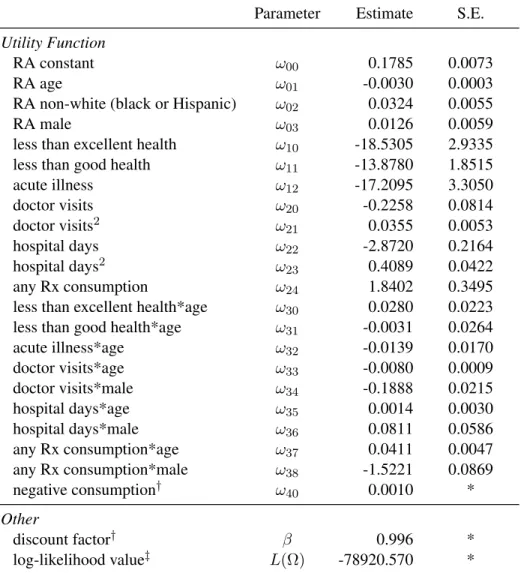
6.1 Preference Parameter Estimates . . . 42

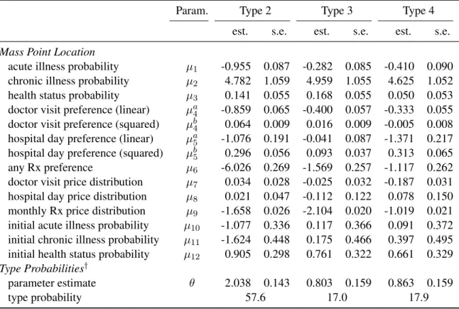
6.2 Permanent Unobserved Heterogeneity Parameter Estimates . . . 43

6.3 Illness Probability Parameter Estimates . . . 44

6.4 General Health Status Probability Parameter Estimates. . . 45

6.5 Observed and Simulated Outcomes . . . 48

6.6 Observed and Simulated Annual Consumption. . . 49

6.7 Predicted Effect of Insurance Possession on Medical Care Expenditure . . . 50

6.8 Other Measures of the Effects of Moral Hazard . . . 52

6.9 Characteristics of the Insured and Uninsured . . . 59

6.10 Predicted Health Insurance Coverage Rate . . . 63

A.1 Representativeness of the Sample . . . 67

A.2 Structural Price Parameter Estimates. . . 68

A.3 Initial Condition Probability Parameter Estimates . . . 69

A.4 Closing Function Structural Parameter Estimates . . . 70

LIST OF FIGURES

3.1 Timing of the Model . . . 11

6.1 Annual Medical Care Expenditure . . . 47

1 INTRODUCTION

Economic theory suggests that health insurance may increase medical care consumption

above the socially optimal level (Arrow 1963; Pauly 1968). The incentives that elicit this

increase in consumption are often referred to as moral hazard (Cutler and Zeckhauser 2000).1

Empirical studies tend to estimate moral hazard effects using models that aggregate

med-ical care decisions up to the annual level. In this dissertation, I study insurance-induced

moral hazard using a dynamic stochastic model of within-year medical care consumption

decisions. The within-year decision-making model more accurately captures the data

gener-ating process by relaxing several assumptions made frequently in the literature. Specifically,

the model allows for endogenous health transitions, variation in medical care prices, and

in-dividual uncertainty within a health insurance year. The research contributes to the literature

in two ways. First, I show that the within-year decision-making model produces a moral

hazard effect that is 24% larger than an alternative model that imposes the more restrictive

assumptions of a typical annual expenditure model.2 _{Second, I provide evidence of}

heteroge-neous moral hazard effects, particularly between insured and uninsured individuals. I explain

why each of these findings is consistent with economic theory and show how differences in

estimated moral hazard effects can lead to large differences in predicted policy outcomes. I

also conduct a series of counterfactual policy simulations to study the potential effects of the

individual insurance mandate provision of the 2010 Patient Protection and Affordable Care

1_{The termmoral hazardis used rather loosely in the health economics literature. I describe moral hazard as}

the incentives associated with insurance possession that lead to changes in individual behavior. I focus on one effect of moral hazard, which is the effect that health insurance possession has on medical care consumption. I discuss the welfare implications of this additional consumption in Appendix D.

2_{The moral hazard effect is measured as the percentage increase in mean annual medical care expenditure}

Act (ACA).

The within-year decision-making model is motivated by theoretical (Grossman 1972;

Keeler, Newhouse, and Phelps 1977) and empirical (Gilleskie 1998; Cardon and Hendel

2001; Khwaja 2001, 2010; Blau and Gilleskie 2008) models of health production and medical

care demand. An individual’s optimization problem consists of an annual health insurance

de-cision, followed by a sequence of monthly medical care consumption decisions made over the

course of a health insurance year. I model monthly medical care decisions to allow the unique

benefits and costs associated with the timing of unexpected illness and potential medical care

consumption to impact behavior within the model. Within each month, a forward-looking

individual responds to an endogenous stochastic health event by consuming units of

medi-cal care. The (anticipated) primary benefit of medimedi-cal care consumption is improved future

health. The (anticipated) primary cost is financial (i.e., a decrease in the current

consump-tion of non-medical goods).3 When health insurance has dynamic cost-sharing features (i.e.,

deductible and stop loss), an additional benefit of current medical care consumption is the

reduced cost of future care once accumulated expenditure crosses a threshold.4 _{The model}

also allows a direct contemporaneous utility benefit or cost of medical care consumption that

is independent of the productive and financial effects.

An individual faces uncertainty along multiple dimensions of the optimization problem.

Prior to both an annual health insurance decision and each monthly medical care decision, an

individual is uncertain of his future health outcomes, medical care consumption, and medical

care prices. Furthermore, I assume that prior to medical care consumption an individual

knows the conditional distributions from which medical care prices are drawn, but does not

3_{I qualifyanticipatedbenefits and costs because the estimated model parameters determine both the sign and}

magnitude of medical care productivity (in producing positive health outcomes) and the disutility from reduced consumption of non-medical goods. I expect to find that medical care is productive, a reduction in non-medical consumption yields disutility, and that each plays a principle role in the medical care decision-making process.

4_{A deductible is a fixed amount of accumulated medical care expenditure that must be reached (within an}

know the exact prices he will be charged for different types of care.5 _{Though it is typically}

assumed that prices are known prior to consumption, there are several reasons why price

uncertainty is a more realistic assumption. First, an individual rarely knows a physician’s

diagnosis and recommended treatment prior to an office or hospital visit. Second, in the U.S.,

medical care providers do not display a menu of prices and there is evidence of wide price

variation in local medical care markets. Each of these market characteristics make it difficult

for an individual to know exactly how much he will be charged for care.

The within-year decision-making model, which is characterized by these important

mar-ket features, also has several empirical advantages. First, the model has the ability to capture

patterns in the data that are explained by within-year behavior. For example, in the

estima-tion sample, average monthly medical care expenditure is $127.60 higher in months where an

individual has an acute illness. This spending gap exists even when conditioning on chronic

illness entering the year: expenditure is $119.78 higher in acute illness months for those

with-out a chronic illness and $140.30 higher for those with a chronic illness.6 This behavior can

be explained by the within-year decision-making model if medical care decreases the

likeli-hood of having an acute illness and has a financial cost. Second, the assumptions imposed

on the within-year decision-making model may impact the estimated effect of moral hazard.

For example, the model allows medical care consumption to affect health over the course of

a health insurance year (i.e., within-year health transitions are treated as endogenous). Most

models of medical care demand either do not model health at all (implicitly assuming that

health transitions are exogenously determined) or model annual health outcomes. Allowing

for endogenous health transitions within an insurance year impacts the estimated effect of

moral hazard if the insured consume more medical care but then find themselves in better

health, decreasing the need for medical care consumption in the future.

5_{I use the termspriceandtotal cost, interchangeably, to describe the total amount billed for a unit of medical}

care. Theout-of-pocket cost to an individual is often less than the price billed due to insurance cost-sharing. The difference between medical care prices and costs paid out-of-pocket is discussed further in Section 3.4.

I estimate the model parameters via maximum likelihood using employer-employee match

data from the 1996-1999 Medical Expenditure Panel Survey (MEPS). I use simulation

tech-niques to examine model fit and to calculate the effect of moral hazard on medical care

expen-diture. I conduct a set of counterfactual simulations to study how different assumptions

im-posed on a within-year decision-making model lead to different moral hazard effects.

Specif-ically, I examine how the estimated effect of moral hazard responds to the assumption that

health transitions are exogenously determined (assumption 1), that medical care prices are

known prior to consumption (assumption 2), and that all health and price shocks are known

at the beginning of the year (assumption 3). The main counterfactual imposes assumptions

1, 2, and 3, as these assumptions are consistent with those made implicitly in most annual

expenditure models, such as Cardon and Hendel (2001), Einav, Finkelstein, Ryan, Schrimpf,

and Cullen (2013), and Kowalski (2013).7

Health insurance is predicted to increase mean annual medical care expenditure by 92%

using the (preferred) within-year decision-making model and 74% when assumptions 1, 2,

and 3 are imposed. The counterfactual estimate compares favorably with estimates produced

by several annual expenditure models in the literature. Ultimately, the presence of health and

price uncertainty at the time of medical care consumption in the preferred model decreases

the expected value of medical care. The larger moral hazard effect produced by the

within-year model is driven by exceptionally low medical care consumption when uninsured, as risk

averse individuals who face uncertainty are exposed to significant risk in consumption.

I find heterogeneous moral hazard effects across the population. The 92% increase in

mean annual medical care expenditure that results from insurance acquisition is driven by

individuals with exceptionally large increases in expenditure. If the top 1% of additional

spenders are dropped, then the increase in mean expenditure due to insurance is reduced to

7_{Bajari, Hong, Khwaja, and Marsh (2013) is similar but does allow for some uncertainty at the time of}

65%. Furthermore, 44% of the population does not increase their expenditure at all when they

become insured. I also find significant differences in how insured and uninsured individuals

respond to coverage. When individuals are moved from an uninsured state to their optimal

plan, mean annual medical care expenditure in the insured population increases by 96%;

however, mean annual medical care expenditure in the uninsured population increases by

only 55%. In Section 6.3.2, I discuss the factors that drive these differences and explore the

policy implications of the differential response to coverage between these two groups.

The dissertation concludes with a counterfactual exercise that examines the behavioral

response to an individual insurance mandate that is consistent with the ACA.8_{When facing a}

penalty of $695 (in 2016 dollars) or 2.5% of income (whichever is larger) for failing to carry

health insurance coverage, the proportion of the population being analyzed that chooses to

be uninsured decreases from 11.8% to 6.0%. Of the previously uninsured population, mean

annual medical care expenditure for the newly insured increases by 77% (moral hazard

ef-fect), while expenditure for those remaining uninsured falls by 2.4% (income/penalty effect).

Given that the full implementation penalty does not elicit universal coverage, I also examine

the welfare implications of forced insurance take-up. Holding insurance premiums and

med-ical care prices fixed, I find that among uninsured individuals the average expected welfare

loss from forced take-up is $1608 (2016 dollars).9

The following section provides motivation for this research and discusses some of the

previous literature. Section 3 details the theoretical model of insurance and within-year

med-ical care demand. Section 4 describes the data and the sample used in estimation. Section 5

details the estimation procedure and discusses identification. Sections 6 presents parameter

estimates, model fit, and counterfactual simulations. Section 7 concludes.

8_{This counterfactual implements the individual mandate provision of the ACA only. There are many other}

regulations that the ACA imposes upon the marketplace that are not considered. Furthermore, the empirical anal-ysis conducted in this research focuses on a population of individuals who are unmarried, childless, employed, between the ages of 19 and 64, and have the ability to purchase health insurance through their employers.

9_{The average expected welfare loss is measured as the average penalty that would make an uninsured}

2 MOTIVATION AND BACKGROUND

Health insurance generates welfare by protecting risk averse individuals from medical

ex-penses associated with unforeseen health shocks (Arrow 1963). However, the welfare gains

from risk protection are potentially mitigated by changes in individual behavior after

becom-ing insured. For example, insurance lowers the out-of-pocket cost of medical care, which

can lead to excess consumption when sick, known as ex-post moral hazard (Pauly 1968).

Also, a reduction in the expected cost of curative medical care can reduce participation in

healthy behaviors (e.g., preventative medical care, diet, exercise, etc.) leading to worse health

outcomes and potentially greater medical care consumption in the future, known as ex-ante

moral hazard (Cutler and Zeckhauser 2000).10 _{Each of these forces drives insured individuals}

to consume medical care past the socially optimal level, generating a welfare loss.11

There-fore, efficient health insurance plan design requires an understanding of how health insurance

leads to changes in individual medical care consumption behavior.

10_{In the empirical health economics literature, moral hazard normally refers only to ex-post moral hazard}

(some exceptions are Dave and Kaestner (2009) and Kelly and Markowitz (2009)). Ex-ante moral hazard is difficult to study for two reasons. First, ex-ante moral hazard involves changes in many non-medical behaviors (i.e., exercise, diet, smoking, etc.). Second, ex-ante moral hazard results from poor health behaviors that lead to worse health outcomes, meaning endogenous health transitions must be modeled. The model presented in this research allows for ex-post moral hazard and limits the effect of ex-ante moral hazard to changes in medical care consumption. That is, an individual in the model may respond to health insurance coverage by consuming medical care less frequently, which may lead to poor health outcomes and greater medical care consumption in the future. However, I do not model non-medical behavioral responses to insurance acquisition.

11_{It is assumed here that the level of medical care consumption when uninsured is socially optimal. If medical}

Determining how medical care consumption and welfare are affected by health insurance

has been a central focus of empirical health insurance and medical care research over the past

30 years. The primary challenge in estimating, for instance, the percentage increase in mean

annual medical care expenditure that is caused by health insurance possession (i.e., a measure

of the effect of moral hazard) is the endogenous selection of health insurance. Those who

expect to consume more medical care during a health insurance year select generous health

insurance coverage; this is known as adverse selection (Akerlof 1970). Both moral hazard and

adverse selection lead to a positive correlation between observed medical care expenditure

and insurance possession/generosity; however, the extent to which this correlation is driven

by moral hazard or adverse selection has important policy implications.12

One method that has been used to control for endogenous insurance selection, so that

moral hazard effects can be identified, is a randomized experiment. A well known

exam-ple is the RAND Health Insurance Experiment (HIE). The 1971 RAND HIE was a

multi-year, $295 million (in 2011 dollars, (Greenberg and Shroder 2004)) medical care study that,

among other things, randomly distributed health insurance plans to participants in 6 U.S.

cities and recorded health and medical care consumption in the years following (for more

details, see Newhouse 1974, 1993). By randomly assigning coverage, the experiment’s

de-sign created exogenous variation in insurance holdings so that price elasticities (i.e., another

measure of the effect of moral hazard) could be estimated. A more recent example of

re-searchers using experimental data to study moral hazard is the Oregon HIE. In 2008, the

Oregon Health Authority expanded the state’s Medicaid program to 10,000 additional

low-income adults using a lottery (i.e., qualifying individuals were randomly selected and given

the ability to apply for coverage). Again, random assignment allows these researchers to

study moral hazard without concern for endogenous insurance selection. This experiment

12_{If moral hazard is the dominant force behind this correlation, then policy makers should encourage less risk}

is ongoing, though one year (Finkelstein, Taubman, Wright, Bernstein, Gruber, Newhouse,

Allen, Baicker, and the Oregon Health Study Group 2012) and two year (Baicker, Taubman,

Allen, Bernstein, Gruber, Newhouse, Schneider, Wright, Zaslavsky, Finkelstein, and the

Ore-gon Health Study Group 2013) evaluations of the program have been published. There are

also numerous quasi-experimental studies that use econometric techniques and exogenous (or

near exogenous) shifts in insurance policy, such as Medicaid expansion (Currie and Gruber

1996; Dafny and Gruber 2005) or the Massachusetts market reforms (Miller 2012; Kolstad

and Kowalski 2012), to control for adverse selection.

While both experimental and quasi-experimental techniques have been used to

success-fully control for adverse selection so that moral hazard effects may be identified, a principle

goal in this literature is to move beyond measuring the spending response to observed plans

and/or policies.13 Recently, research efforts have focused on measuring the welfare

implica-tions of the additional spending caused by moral hazard and designing insurance plans and

insurance plan alternative sets that improve consumer welfare. In this pursuit, researchers

have turned to structural modeling.14 _{Importantly, structural models have allowed researchers}

to both control for adverse selection in order to quantify moral hazard effects and to

calcu-late the welfare implications of these effects. Furthermore, because insurance decisions are

typically modeled and insurance cost-sharing characteristics are allowed to impact optimal

13_{The experimental and quasi-experimental research found in this literature has generally focused on}

analyz-ing the effects of specific policies on outcomes of interest. Unfortunately, these results are difficult to generalize, as the estimated effects are normally applicable for only a specific policy and population. Manning, Newhouse, Duan, Keeler, and Leibowitz (1987) and Keeler and Rolph (1988) are exceptions to this rule, as they estimate a single price/co-insurance elasticity of medical care demand that is frequently used by researchers and policy makers to predict changes in medical care expenditure levels that would result from insurance plans and policies not observed in the marketplace. However, as is discussed extensively in Aron-Dine, Einav, and Finkelstein (2013), application of the single price elasticity measure requires a researcher to characterize a health insurance plan by a single price. Because modern health insurance plans are characterized by many cost-sharing features that change the out-of-pocket cost of medical care over the course of a health insurance year, there is no obvious way to summarize a plan by a single price. Aron-Dine et al. (2013) conduct an empirical exercise where they predict medical care expenditure using the single price elasticity and implement several common strategies for determining a single price. Their results show wide variation in predicted results depending on the strategy used.

14_{In this context, structural modeling should be interpreted as explicitly modeling and estimating the}

medical care decision making through the budget constraint, the models are well suited to

study behavioral and welfare responses to counterfactual insurance plans, insurance

alterna-tive sets, and regulatory policies.

Among the related structural models that have been designed and estimated (Cardon and

Hendel 2001; Khwaja 2001, 2010; Einav et al. 2013; Kowalski 2013; Bajari et al. 2013;

Hdel 2013), all have aggregated medical care expenditures and health outcomes up to the

an-nual level.15 Annual expenditure models have been popular, here and elsewhere in the health

economics literature, primarily due to data limitations. Annual medical care expenditure data

are accessible. Large public data sets, which contain total annual expenditure variables that

have been cleaned and are ready for immediate use, are used by many empirical researchers

and allow for nationally representative findings.16 _{Also, estimation of annual expenditure}

models can be achieved without high frequency explanatory data, such as illness state, which

is both difficult to find and desirable when estimating a model of within-year medical care

decisions.17 My research builds on these structural annual expenditure models by allowing

for monthly medical care consumption decisions to be made over a health insurance year and

by relaxing several assumptions commonly made in annual decision-making models.18

15_{Khwaja (2001, 2010) aggregates to the biennial level.}

16_{Examples are: the Medical Expenditure Panel Survey (MEPS); the Health and Retirement Survey (HRS),}

which has been cleaned by RAND; and the Medicare Current Beneficiary Survey (MCBS).

17_{Note that while insurer claims data (or claims data from a large self-insuring company, which are used}

in Einav et al. 2013; Kowalski 2013; Bajari et al. 2013; and Handel 2013) allow for the observation of high-frequency medical care consumption decisions, illness state is only observed when an individual chooses to consume care. Therefore, endogenous health transitions cannot be modeled well using claims data.

18_{A few researchers have studied health insurance and/or medical care demand using within-year behavior}

3 MODEL

This section describes the optimization problem solved by an unmarried, childless,

em-ployed individual who makes an annual health insurance decision followed by a sequence of

medical care consumption decisions to maximize the value of his expected discounted future

utility.19 The timing of the model can be observed in Figure 3.1. At the beginning of each

year,y, a forward-looking individual observes the set of health insurance alternatives offered

by his employer, his general health status, and the presence of any illnesses. Before the start

of the first month, t = 1, he chooses the health insurance alternative that maximizes his

ex-pected discounted future utility. Among other things, this exex-pected utility is a function of

anticipated medical care behavior within the year conditional on insurance coverage. In this

research the within-year medical care behavior is modeled explicitly.

At the beginning of each month, an individual learns his illness state, which evolves

stochastically over the course of the year and is influenced by his general health status, illness

history, and previous medical care consumption. After learning his current illness state, the

individual decides how much (and what types of) medical care to consume. The amount he

pays for a unit of medical care depends on the unit price, the cost-sharing characteristics of

his health insurance plan, and his accumulated medical care expenditure within the coverage

year. Much like the price uncertainty individuals face in the US medical care market, the

total price of care is stochastic over time and unknown prior to consumption. After making a

19_{The model features employed individuals who receive an employer-sponsored health insurance offer (ESHI)}

Figure 3.1: Timing of the Model

y

Annual health insurance decision

t = 1 t= 2

Monthly medical care decisions Each month:

(1) Learn illness state

(2) Select among medical care alternatives (3) Observe updated general health status

t= 12

y+ 1

medical care decision, the individual’s general health status evolves prior to the next month.

The remainder of this section explains the model and solution in greater detail.

3.1 Annual and Monthly Decisions

At the beginning of each year, an individual observes the set of health insurance plans

available to him from his employer. Each plan is defined by its premium, network type, and a

set of cost-sharing characteristics. The cost-sharing features enter an individual’s budget

con-straint throughout the year, determining how much is paid out-of-pocket for medical care. The

following plan characteristics enter the model: out-of-pocket premium, composite annual

de-ductible, doctor’s office dede-ductible, hospital dede-ductible, stop loss, hospital co-insurance rate,

hospital co-pay level, doctor’s office co-insurance rate, doctor’s office co-pay level,

physicians (HMO, PPO, or FFS).20 _{An indicator function,I}j

iy, equals one if individuali

se-lects insurance planj in yearyand zero otherwise.21 _{Only one plan can be held at a time, so}

that

X

j∈Ji

I_iyj = 1 ∀i∀y (3.1)

whereJi _{is the set of exogenously determined employer-sponsored health insurance (ESHI)}

plans and includes the option to decline all plans.22

In each month, an individual learns his illness state (defined below) before making a

medical care consumption decision. He chooses the number of doctor visits, vit; hospital

days,sit;23and whether or not to consume prescription drugs,rit.24 The monthly medical care

decision is represented by an indicator function,dvsr

it , that equals one if an individual chooses

the bundle (v, s, r)and zero otherwise. Bundles are mutually exclusive with a maximum of

20_{A deductible and a stop loss are described in footnote 4. A co-insurance rate is the share of the medical}

care price that an individual must pay out-of-pocket (the remainder is paid by the insurer). A co-pay level is a fixed dollar amount that an individual must pay out-of-pocket for a unit of medical care (again, the remainder is paid by the insurer). A health maintenance organization (HMO) here refers to an insurance plan that limits its enrollees to receiving medical care from a specified group of providers. A preferred provider organization (PPO) is a plan that defines a preferred network of providers from which care can be purchased less expensively. If an enrollee chooses to seek care outside of this network, coverage is still provided but at a higher out-of-pocket cost. A fee-for-service (FFS) plan covers an enrollee equally at all medical care providers.

21_{For notational simplicity and consistency, I include the subscripti to describe individual level variables}

only when defining the variable. The subscriptiis suppressed thereafter.

22_{Some individuals select a job based (at least partially) on the health insurance offered. However, modeling}

an individual’s decision to accept a particular job, with health insurance options as a job characteristic, requires modeling the employment decision as a function of health insurance characteristics. Thus, this exogeneity assumption has become the norm in the literature.

23_{Hospitaldaysare chosen rather than the standard (hospital)nightsbecause inpatient and outpatient hospital}

visits are not modeled separately. A visit to the ER and an outpatient procedure each constitute a decision to consume one hospital day. A single overnight visit reflects a decision to consume two hospital days.

24_{According to the Centers for Disease Control and Prevention (CDC) these three types of care account for}

V doctor visits andShospital days each month, such that

V

X

v=0

S

X

s=0 1

X

r=0

dvsr_it = 1 ∀i∀t. (3.2)

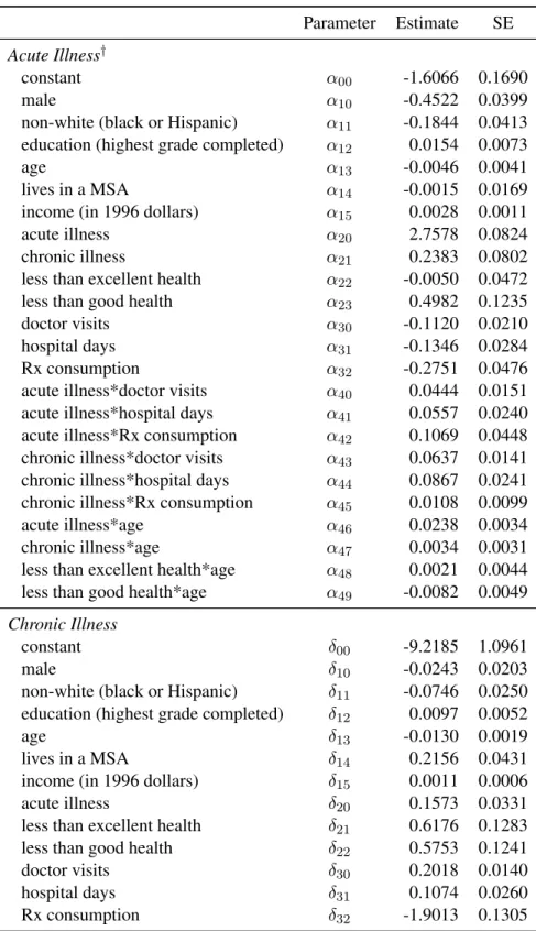
3.2 Health Transitions and Probabilities

Three measures of individual health evolve stochastically over the course of the insurance

year. The acute illness state, Ait = {0,1}, and the chronic illness state, Cit = {0,1}, are

dichotomous. General health status, Hit, takes on one of three values: excellent (Hit = 2),

good (Hit = 1), or poor (Hit = 0).25

I define an acute illness as any medical condition that eventually subsides and, under

normal conditions, has no permanent effect on an individual’s health or medical care

con-sumption. This characterization describes both short-natured ailments, such as a common

cold or influenza, as well as non-permanent but persistent conditions, such as a pneumonia or

a broken bone. In estimation, the probability that an individual is in an acute illness state in

monthtis determined by a logistic function such that

P(At = 1) =πt1 =

exp(α0+α1Wt+α2HAt +α3Mt−1+α4NAt +µk1)

1 +exp(α0+α1Wt+α2HAt +α3Mt−1+α4NAt +µk1)

(3.3)

where Wt contains demographic factors such as sex, race, income, education, MSA

indi-cator, age, and month indicators; HA_t is general health status and illness state entering the

month (1Ht<2,1Ht<1, At−1, Ct−1); Mt−1 is medical care consumption in the prior month

(vt−1, st−1, rt−1); NAt contains interactions of the variables in (Wt,HAt ,Mt−1); and µk1

captures unobserved permanent individual heterogeneity for an individual of typek, where

k = 1, ..., K.26 _{Interactions are used to allow the effect of medical care to vary by illness}

25_{Death is only observed once in the data because the estimation sample includes ages 19-64, so it is not}

modeled as a possible health outcome. Adeath statewould be a simple addition with alternative data sets.

26_{See Section 5.1 for a discussion of estimation and interpretation of unobserved permanent individual}

state entering the month.

I define a chronic illness to be any medical condition that never subsides (e.g., diabetes,

asthma, AIDS) or, under normal conditions, has a permanent effect on an individual’s health

or medical care consumption (e.g., cancer, stroke, hypertension).27 _{Given the long-lasting}

effect of these ailments on health and/or medical care purchasing behavior, the occurrence

of a chronic illness is modeled as a permanent, absorbing state. However, medical care can

be used to control a chronic illness so that it has a lesser negative impact on an individual’s

general health status and acute illness probability. I model the probability that an individual

is in a chronic illness state in monthtas a logistic function such that

P(Ct = 1) =γt1 =

   

  

exp(δ0+δ1Wt+δ2HCt +δ3Mt−1 +δ4NCt +µk2)

1 +exp(δ0+δ1Wt+δ2HCt +δ3Mt−1+δ4NCt +µk2)

if Ct−1 = 0

1 if Ct−1 = 1

(3.4)

whereHC_t = (1Ht<2,1Ht<1, At−1). 28

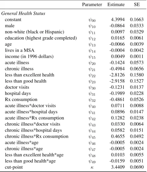
At the end of each monthtan individual’s general health status is updated, Ht+1, before

transitioning to the next month t+ 1. Motivation for the inclusion of general health status

comes from the household production approach of Grossman (1972), who describes both a

27_{This definition classifies several permanent physiological conditions as chronic illnesses that are not}

typi-cally categorized as such, because the conditions are likely to impact an individual’s future medical care con-sumption (e.g., amputations, menopause, organ and joint replacement).

28_{The MEPS data classifies illness by ICD-9-CM condition codes, which would allow for a more detailed}

consumption motive and a production motive for the utilization of medical care. In

Gross-man’s model, an individual consumes medical care to rebuild an ever depreciating stock of

health. The health stock produces health flows (e.g., healthy days), which directly increase

utility and can be used to produce income or other consumption goods. The model presented

in this research takes a similar approach by allowing general health status to enter the utility

function and by allowing general health status to be influenced by past health and medical

care consumption. I assume general health status has the following ordered structure

H_t∗₊₁ =ψ0+ψ1Wt+ψ2HHt +ψ3Mt+ψ4NtH+µk3+ζt+1

and Ht+1 =

      

     

2 if κ < H_t∗₊₁

1 if 0< H_t∗₊₁ ≤κ

0 if H_t∗₊₁ ≤0

(3.5)

where H_t∗₊₁ represents latent general health, HH_t = (1Ht<2,1Ht<1, At, Ct), andκ is a

cut-off point to be estimated. Assuming ζt+1 follows a logistic distribution, the (ordered logit)

probability of transitioning to each general health level is

P(Ht+1 = 2) =ηt2+1 = 1−Λ(κ−ψZt)

P(Ht+1 = 1) =ηt1+1 = Λ(κ−ψZt)−Λ(−ψZt)

P(Ht+1 = 0) =ηt0+1 = Λ(−ψZt)

(3.6)

whereψ = (ψ0, . . . , ψ3, µk3), Zt = (Wt,HHt ,Mt,NHt ), and Λ(·)is the logistic function. In

addition to its theoretical relevance, general health status plays an important role in this model

because it gives purpose to medical care consumption when in a chronic illness state, which

is important given that chronic illnesses never expire. Through interactions, this specification

allows medical care consumption to alter the effect that a chronic illness state has on general

to lessen the negative impact of the disease on his general level of health - not tocurethe

dis-ease. The same could be said of open heart surgery, blood-pressure medication, or asthmatic

inhalers.

3.3 Utility Function and Budget Constraint

Preferences for a medical care consumption bundle (vt = v, st = s, rt = r)in month t

are described by the following contemporaneous utility function29

U(Xt, R,HUt , d

vsr t , µ

k

, vsr_t ) = X ω0R

t

ω0R

+ω1HU_t +ω2MU_t +ω3NU_t +µ₄k_v+µk_5s+µk_6r+vsr_t

=U(dvsr_t ) +vsr_t

(3.7)

where Xit represents consumption of non-medical goods (determined by the budget

con-straint defined in Equation 3.8); R = (1, sex, race, age); HU

t = (1Ht<2,1Ht<1, At, Ct);

MU_t = (vt, st, rt, vt2, s2t); NUt contains interactions of the variables in(HUt ,MUt ,Wt); the

µkparameters capture unobserved permanent heterogeneity for an individual of typek; and

vsr_it is the unobserved utility received from v doctor visits,s hospital days, and consuming

prescription drugs(r = 1)or not(r= 0).30

The monthly budget constraint is

Xt =Yt−Pjt−Ot(vt, st, rt, pvt, pst, prt, ADEt, AHEt, Iyj) (3.8)

whereYitis monthly income;Pijtis the monthtpremium paid out-of-pocket for planj;Ot(·)

29_{This utility function is representative whenXtis greater than or equal to zero. If medical care expenditure}

becomes so great thatXtis negative, then the first term X

ω0R t

ω0R is replaced byω40∗Xtto capture the (dis)utility

of negative non-medical good consumption.

30_{I allow the effect of unobserved permanent individual heterogeneity in the utility function to vary by}

is the out-of-pocket expenditure on medical care in month t; pv

it, psit, and prit represent the

total price of a doctor visit, a hospital day, and prescription drugs, respectively; andADEit

and AHEit represent accumulated out-of-pocket medical care expenditure for doctor visits

and hospital days entering montht, respectively.31 _{This structure assumes that an individual}

consumes all income by the end of each month, as monthly saving decisions are not observed

in the data.32

Having specified the contemporaneous utility function, budget constraint, and all

transi-tions between uncertain illness states and general health status, I denote the set of information

known by an individual at the time of a medical care consumption decision, or hisstate, as

Ψt = (Wt, Ht, At, Ct, ADEt, AHEt, Iyj, µk, vsrt ). It remains to describe what the model

as-sumes about an individual’s knowledge of medical care prices and out-of-pocket expenditure;

then, the optimization problem can be fully expressed.

3.4 Medical Care Prices and Expenditure

Two characteristics of the medical care marketplace make within-year medical care

ex-penditure an important economic construct. First, most individuals do not pay the total price

of medical care because of a cost-sharing arrangement with their health insurance provider.33

Rather, an individual pays a dollar amount out-of-pocket that is determined by the total price

of medical care, insurance plan characteristics, and accumulated medical care expenditure

31_{Because an individual faces a binary decision on whether or not to consume any prescription drugs,p}r itis a

total monthly expenditure on prescription drugs rather than the unit price per prescription.

32_{French and Jones (2011) examine the effects of health insurance and self-insurance (i.e., savings) on}

re-tirement behavior. The authors explain that omitting savings from an individual’s dynamic problem ignores the ability to smooth consumption through savings, which can potentially overstate the value of insurance. In simulation, they find that omitting savings from the model does increase the value of insurance, but (retirement) decision making is unchanged in the no-savings model.

33_{Medical care can be thought of as having two prices, alistprice and a transactionprice. The list price}

during the coverage year. For example: an individual with a $300 deductible, 10%

co-insurance rate, and $0 of accumulated expenditure who is charged $100 for a doctor visit

pays the full $100 out-of-pocket. However, if the same individual were to have accumulated

$250 in medical care expenditure prior to the visit, then he would pay only $55 out-of-pocket

for the visit ($50 pre-deductible+ $5 [= 0.1∗($100−$50)]post-deductible). An individual

with health insurance characterized by this cost-sharing structure (i.e., a deductible with a

co-insurance rate) faces a non-linear budget constraint. The out-of-pocket expenditure

func-tion, Ot(·), is constructed so that the budget constraint in Equation 3.8 contains these

non-linearities. Precise calculations of out-of-pocket expenditure and accumulated out-of-pocket

expenditure are detailed in Appendix C.

A second characteristic of the medical care market is that individuals are typically

uncer-tain of the total price of medical care prior to consumption. The lack of menu prices,

un-certainty of diagnosis prior to a visit, and wide price variation in local medical care markets

contribute to price uncertainty.34 Despite the evidence, surprisingly few models of medical

care demand allow for this uncertainty. To address this reality, I assume that an individual

does not observe total medical care prices prior to making a medical care decision in each

month. Rather, an individual knows the conditional distributions from which doctor visit

prices, hospital day prices, and prescription drug prices are drawn. An individual makes

medical care decisions by integrating over the three conditional price distributions, which are

estimated from the data.35

The total price distributions are defined asFv_(pv

t|Φt;λv),Fs(pst|Φt;λs), andFr(ptr|Φt;λr),

whereΦt = (Wt, Ht, At, Ct, HM Oj, P P Oj, F F Sj, µk)is a vector of variables that explain

34_{In May 2013, the Centers for Medicare and Medicaid Services (CMS) released data showing wide variation}

in medical care prices in local medical care markets. Such variation makes it difficult for an individual to know medical care prices prior to consumption. Recent articles in Time Magazine and The New York Times have also highlighted the issue of price uncertainty in medical care markets.

35_{An equilibrium model of the medical care market could conceivably allow for price determination in}

variation in the distributions and (λv_{, λ}s_{, λ}r_{) are parameters to be estimated. The variables}

HM Oj, P P Oj, and F F Sj are indicators of the plan’s coverage type. Coverage type is

in-cluded to capture the negotiation for lower rates by insurance providers who contract with

a network of physicians.36 _{An indicator of MSA level is included in W}

t to capture urban

area variation in prices. In addition to differences attributed to supply side variation, these

distributions depend on individual observed illness states and general health status. Finally,

these medical care price shocks are likely to be correlated with unobserved illness and health

shocks. An individual who receives an exceptionally bad illness shock (e.g., cancer) is also

likely to experience a price distribution that is shifted upward or has fatter tails. For this

rea-son, the three medical care price shocks are likely to be correlated with one another as well.

I allow the permanent unobservables that influence preferences, illness states, and general

health outcomes to also influence the price distributions. Currently, the model does not allow

for time-varying unobserved heterogeneity.

3.5 The Optimization Problem

An individual’s objective is to maximize his expected discounted future utility by

select-ing the optimal sequence of medical care bundles,dvsr

t , fort = 1, ..., T and insurance plans,

I_yj, fory= 1, ...Y conditional on his state variables inΨt. I describe an individual’s dynamic

optimization problem in two stages, as insurance decisions are made at the beginning of a

year and medical care is chosen repeatedly over the course of a year.

3.5.1 The Optimal Monthly Decision Rule

Let Vach

vsr (·t) be the montht value of expected discounted future utility for medical care

decision dvsr

t , illness state (At = a, Ct = c), and general health status (Ht = h). Using

Bellman’s Equation (Bellman 1957), this value is constructed as the sum of contemporaneous

36_{The model does not differentiate between in-network and out-of-network medical care consumption. All}

utility and the expected discounted future utility yielded by the alternative. Conditional on

unobserved heterogeneity type k (whereµk _{= {µ}k

1, ..., µk14}), insurance planj, and medical

care prices (pv_t,ps_t,pr_t), the alternative-specific value function can be written, fort < T

V_vsrach(Ψt, vsrt |µ k

, I_yj, pv_t, ps_t, p_tr) = U(dvsr_t ) +vsr_t

+β 2

X

h0₌₀ "

η_th₊₁0 (Ψt, dvsrt )

1

X

a0₌₀

πa_t+10 (h0,Ψt, dvsrt )

1

X

c0₌₀

γ_tc₊₁0 (h0,Ψt, dvsrt )

h

Va0c0h0(Ψt+1|µk, Iyj)

i #

,

(3.9)

and fort=T

V_vsrach(Ψt, vsrt |µ k

, I_yj, pv_t, ps_t, pr_t) = U(dvsr_t ) +vsr_t +β 2

X

h0₌₀ h

η_th₊₁0 (Ψt, dtvsr) [Qy+1(Ψ0, h0)]

i

(3.10)

whereU(dvsr

t )is the deterministic part of Equation 3.7,βis the discount factor, andQy+1(Ψ0, h0)

is the value of expected discounted future utility in montht = 0of yeary+ 1. Maximal

ex-pected utility, in illness state(At+1 =a0, Ct+1 = c0)with general health status(Ht+1 = h0),

in montht+ 1is

Va0c0h0(Ψt+1|µk, Iyj) =Et

h max

vsr V a0_c0_h0

vsr (Ψt+1, vsrt+1|µ

k_{, I}j y)

i

. (3.11)

The expectation operator is subscripted bytbecause an individual must form this expectation

prior to learning montht+ 1medical care preference shocks,vsr_t+1.

The value function in Equation 3.9 is written conditional on realized medical care prices.

However, it is assumed that an individual does not know the prices of the three types of

medical care prior to consumption; rather, he knows the conditional distributions from which

price distributions. The value function, unconditional on prices, is

V_vsrach(Ψt, vsrt |µ k

, I_yj) = Z

R3+

f∗(pv_t, ps_t, p_tr)V_vsrach(Ψt, vsrt |µ k

, I_yj, pv_t, ps_t, p_tr)dpv_tdps_tdpr_t (3.12)

wheref∗(pv

t, pst, prt) =fv(pvt)∗fs(pst)∗fr(prt)andfv(·),fs(·), andfr(·)are the conditional

density functions from whichpv

t,pst, andprt are drawn.37

Conditional on the prior insurance decision and unobserved heterogeneity, a utility

maxi-mizing individual selects each medical care consumption bundle with probability

P(dvsr_t = 1) =P hV_vsrach(Ψt, vsrt |µ k_{, I}j

y)≥V ach

v0_s0_r0(Ψ_t, v 0_s0_r0

t |µ k_{, I}j

y) ∀ v

0

s0r0i . (3.13)

3.5.2 The Optimal Annual Decision Rule

The problem can be solved backwards to recover the time t = 0, year yvalue function

conditional on any chosen health insurance alternativej ∈Ji

y. That is,

V(Ψ0, H1 =h|µk, Iyj) =

1

X

a=0

πa₁(Ψ0, H1) 1

X

c=0

γ₁c(Ψ0, H1)

Vach(Ψ1|µk, Iyj)

. (3.14)

Stated explicitly, Equation 3.14 represents the discounted value of optimal future behavior

calculated at the beginning of yearyunconditional on the first month acute and chronic illness

state but conditional on general health status entering the year and insurance planj (i.e., the

expected discounted future value of planj).38 _{This value does not completely determine the}

optimal insurance alternative, as an individual may have preferences for unobserved insurance

characteristics.39 Therefore, I allow further variation through an additive error term such that

37_{Conditional onµ}k _{(unobserved permanent individual heterogeneity) these distributions are independent;}

however, their dependence onµk allows some correlation.

38_{Notice that general health status in month 1,H}

1, is already known at this time because it was learned during the last month of the prior year.

39_{Unobserved characteristics could be defined coverage restrictions, such as a preexisting condition clause}

the expected discounted future value of planj is

Qj_y(Ψ0, H1, φjy|µ k

) = V(Ψ0, H1|µk, Iyj) +φ j

y . (3.15)

A utility maximizing individual selects each insurance plan with the probability40

P(I_yj = 1) =P hQj_y(Ψ0, H1, φjy|µ k

)≥Qj_y0(Ψ0, H1, φj

0

y|µ k

) ∀j0i . (3.16)

This optimization problem is consistent with our theoretical understanding of insurance

benefits. Health insurance is valuable because it provides risk protection, allows for higher

non-medical consumption when ill, and yields health benefits if additional medical care is

consumed during a coverage year. Further, the model explicitly captures the non-linear

re-lationship between a plan’s expected value at the beginning of a year, its cost-sharing

char-acteristics, and an individual’s uncertainty about his future health, medical care prices, and

medical care demand.

that are unlikely to alter the value of a plan during the year but influence individual decisions, such as the plan’s order on the application file or brand name. Choice inertia, or the tendency of individuals to simply select the same health insurance plan that they had in the previous year, is another unobserved factor that may influence an individual’s observed plan. Handel (2013) finds evidence of substantial inertia in the dynamic insurance decisions of employees at one large American firm.

40_{In the optimization problem, an individual has knowledge ofΨ}

4 DATA

My empirical analysis uses data from the 1996-1999 cohorts of the Medical Expenditure

Panel Survey (MEPS).41 MEPS contains detailed health, medical care expenditure, health

insurance, and demographic information for a nationally representative sample of families

and individuals in the United States. New participants are added annually (beginning in 1996

through the present day), drawn randomly from the previous year’s National Health Interview

Survey sample. Individuals in each cohort are interviewed 5 times over the 2 years that follow

January 1st of their cohort year.

The MEPS has two features that make it particularly well suited for the purposes of this

re-search. First, detailed employer level insurance information that can be linked to the

individ-ual file was collected for the 1996-1999 cohorts. Data collectors used information gathered in

the first interview to contact current main employers, from which they obtained premium and

cost-sharing characteristics for all plans offered to the employee. This data feature, which is

unique in national survey data, enables me to model a health insurance decision from the full

set of available alternatives for individuals with participating employers. However, roughly

50%of individuals participating in MEPS are without insurance information in thislink file

due to employee and/or employer refusal to reveal information.42 _{Also, while individuals are}

41_{The data are collected and maintained by the Agency for Healthcare Research and Quality (AHRQ). All}

data used in estimation are publicly available, with the exception of the individual insurance plan information. These restricted files may only be accessed through a Census Bureau Research Data Center (RDC).

42_{There was one significant change to the collection process that took place after 1996. The 1996 MEPS asked}

interviewed over the course of two years, few employers agree to provide health insurance

plan information at the beginning of each year. Therefore, analysis concentrates on one health

insurance decision and the medical care decisions in the year that follows for each

individ-ual. Second, unlike claims data, the MEPS allows participants to report illness episodes even

when they choose not to consume medical care. This data feature allows endogenous illness

transitions to be modeled.

A number of important assumptions are required to prepare the data for estimation. For

example, each illness, which is defined in the data by an ICD-9-CM medical code, must be

interpreted as an acute or chronic illness. Also, medical care consumption dates and partially

observable illness dates must be used to determine the starting and ending month of illnesses

reported five times over the course of 2 years. I also face the challenge that at least one of

the 12 insurance cost-sharing features is missing in 47% of the 5284 plans observed in the

data, so imputations must be made. The magnitude of these complications, and others, and

the assumptions required to overcome them are discussed at length in Appendix B.

4.1 Determination of the Sample

The sample used in estimation is taken from the nationally representative sample of single

and childless individuals included in the 1996-1999 cohorts of the MEPS survey. (See Table

4.1 for sample size by cohort year and inclusion criteria.) I focus on employed individuals

be-tween the ages of 19 and 64 whose employers sponsor health insurance coverage.43 I exclude

the unemployed and those employed without an insurance offer because only general

insur-ance information was gathered for these individuals (e.g., coverage status, coverage source,

etc.). Employed individuals who receive an insurance offer but choose to be uninsured are

in-cluded in the estimation sample. These omissions are representative of the sample restrictions

43_{I study individuals over 18 years old to avoid the unique decision-making process of an adolescent with}

found in similar work.44

Sample inclusion also requires that the ESHI plans that are offered to an individual are

observed in the link file described above. The information contained in the link file is

nec-essary to model an individual’s insurance decisions. Individuals must also participate in all

interviews during the insurance year. The final restriction limits individuals in the sample to

one of two types: (1) individuals taking up ESHI, holding it for an entire year, and holding no

outside coverage; or (2) individuals remaining completely uninsured all year. I do not model

insurance switching during an insurance year and cannot observe privately purchased plan

characteristics.

Table 4.1: Sample Inclusion Criteria

1996 1997 1998 1999 Total

1996-1999 MEPS Household Component 22601 13683 11137 14178 61599

and single, childless, 19-64 yrs old 4406 2534 2169 2589 11698

and employed in first interview period with offer 1821 923 987 1128 4859

and matches to link file† 749 516 159 688 2112

and no missing interviews 693 472 139 636 1940

and stable insurance status 455 290 98 389 1232

†There is a disproportionate drop in link file matches in 1998 because AHRQ only attempted to contact employers for 25% of survey participants who reported being offered health insurance coverage. In all other years, AHRQ attempted to contact employers for all of these individuals.

The final estimation sample contains 1232 individuals (or 14784 person-month

observa-tions). Table A.1, which can be found in Appendix A, compares the 4859 individuals

remain-ing at line 3 above (which is a nationally representative sample of sremain-ingle, childless, 19-64

year olds, who are employed and offered health insurance from their employer) and those

in the estimation sample. The table reveals few differences between the estimation sample

and a nationally representative sample of this demographic. The estimation sample is slightly

44_{Cardon and Hendel (2001) limit their sample to single, childless, employed individuals who are between}

older, a little wealthier, and is comprised of a larger proportion of females. These differences

contribute to higher medical care expenditure in the estimation sample. The estimation

sam-ple is also comprised of more federal employees, which is expected, as no federal employees

are excluded due to employer non-response.

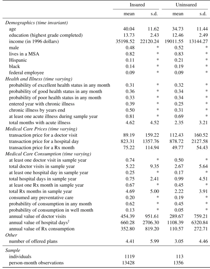
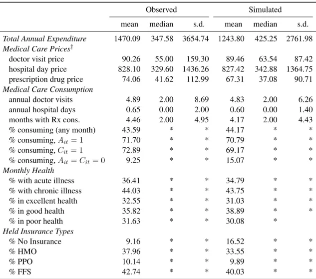
4.2 Sample Statistics

The following tables summarize the mean and dispersion of key variables used in

estima-tion. Table 4.2 compares insured and uninsured individuals in the estimation sample.45 _The

insured are older, more educated, and wealthier. They are also more likely to be white and

female. The insured are more likely to enter the insurance year with a chronic illness, are

more likely to get an acute illness at some point during the insurance year, and have more

months where some acute illness is experienced. The insured also consume more units and

greater values of doctor and prescription drug care.46 The percentage of the population that

consumes at least one hospital day during the year (25% of insured and 17% of uninsured

in-dividuals) seems large, but includes emergency room visits as well as outpatient and inpatient

visits. To improve estimation time, I limit the maximum number of doctor visits and hospital

days in a month (V and S from Equation 3.2) to 9 and 5, respectively.47 _{The insured face}

lower (total) prices for doctor visits and hospital days and higher prices for prescription drugs.

45_{Most variables are self-explanatory. Income is calculated as the sum of post-tax income, sale earnings, and}

tax refund. General health status is self-reported, taken from the response to the question “In general, compared to other people of your age, would you say that your health is excellent, good, fair, poor, or very poor?” Roughly 6% of the estimation sample reports poor or very poor health, so the lowest three health categories (fair, poor, and very poor) are combined to form the poor general health statuscategory seen in the table and used in estimation. Medical care prices are only observed when medical care is consumed. For more detail on medical care prices, medical care consumption, and illness occurrence see Appendix B.

46_{While the uninsured are less likely to have at least one hospital day, the average number of hospital days}

for the uninsured is greater than that of the insured. This is likely due to emergency room usage among the uninsured.

47_{Of the 14,784 person-month observations in the data, the number of doctor visits exceeds the maximum of}

Table 4.2: Sample Statistics by Insurance Status

Insured Uninsured

mean s.d. mean s.d.

Demographics (time invariant)

age 40.04 11.62 34.73 11.44

education (highest grade completed) 13.73 2.43 12.46 2.49

income (in 1996 dollars) 35198.52 22120.24 19011.55 13144.27

male 0.48 * 0.52 *

lives in a MSA 0.82 * 0.83 *

Hispanic 0.11 * 0.21 *

black 0.14 * 0.19 *

federal employee 0.09 * 0.09 *

Health and Illness (time varying)

probability of excellent health status in any month 0.31 * 0.32 *

probability of good health status in any month 0.36 * 0.34 *

probability of poor health status in any month 0.33 * 0.34 *

entered year with chronic illness 0.39 * 0.25 *

chronic illness by years end 0.50 * 0.31 *

at least one acute illness during sample year 0.81 * 0.69 *

total months with acute illness 4.62 4.52 2.35 3.21

Medical Care Prices (time varying)

transaction price for a doctor visit 89.19 159.22 112.43 160.52

transaction price for a hospital day 823.31 1357.76 878.72 2127.58

transaction price for a Rx month 75.22 114.94 49.77 54.43

Medical Care Consumption (time varying)

at least one doctor visit in sample year 0.74 * 0.50 *

total doctor visits in sample year 5.22 9.35 2.67 5.64

at least one hospital day in sample year 0.25 * 0.17 *

total hospital days in sample year 0.75 2.41 0.99 4.51

at least one Rx month in sample year 0.67 * 0.45 *

total Rx months in sample year 4.69 5.00 2.22 3.91

consumed any preventative care 0.20 * 0.19 *

probability of consumption in any month 0.62 * 0.45 *

probability of consumption in well month 0.13 * 0.05 *

annual value of doctor visits 454.39 951.61 289.67 759.21

annual value of hospital days† 660.28 2706.30 1108.39 6320.84

annual value of Rx consumption 352.80 819.20 110.57 272.71

Other

number of offered plans 4.41 5.99 3.05 4.46

Sample

individuals 1119 113

person-month observations 13428 1356

Table 4.3: Insurance Plan Summary

Held Plans Rejected Plans

plans mean s.d. plans mean s.d.

Premium

total premium 1119 2057.19 819.09 4165 2207.13 715.25

out-of-pocket premium 1119 343.83 540.31 4165 519.46 610.28

Deductible†

defined by total expenditure 397 283.59 272.99 772 293.25 348.26

defined by doctor expenditure only 59 191.38 97.04 655 215.72 50.65 defined by hospital expenditure only 28 252.63 218.10 62 150.58 41.24

plan has no deductible 648 * * 2684 * *

Stop loss

stop loss 729 1512.82 1077.97 2775 1689.06 1077.63

plan has no stop loss 390 * * 1390 * *

Hospital‡

co-insurance rate 417 17.02 9.91 797 15.44 8.01

co-pay level (per stay) 199 258.46 346.70 768 159.41 194.45

co-pay level (per day) 85 52.61 60.25 142 58.70 85.24

free care past the deductible 435 * * 2577 * *

Doctor

co-insurance rate 208 18.91 8.69 755 12.43 7.83

co-pay level 858 10.19 4.53 3110 8.41 4.25

free care past the deductible 53 * * 300 * *

Network Type

HMO 1119 0.42 * 4165 0.51 *

FFS 1119 0.47 * 4165 0.44 *

PPO 1119 0.11 * 4165 0.06 *

†These categories are not mutually exclusive. Some of the plans that feature a doctor specific deductible also feature a hospital specific deductible.

The large variance in prices is due to the broad classification of medical care consumption

types. High priced procedures (e.g., outpatient hospital surgery) and low priced procedures

(e.g., emergency room visit for a sprained ankle) contribute to the same price distribution. An

individual is considered to haveconsumed any preventative careif during the sample period

they consume any form of medical care in a month in which they have no acute illness or

chronic illness.

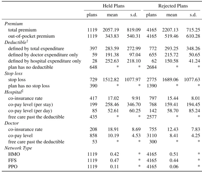
Differences between the chosen and rejected plans can be observed in Table 4.3. The

table suggests that individuals have a general preference for lower premium and therefore

less generous (in terms of cost-sharing features) plans. Compared to the average rejected

plan, held plans are more likely to have a deductible, less likely to have a stop loss, and set

higher thresholds when the plan has a deductible or stop loss. Held plans also feature higher

co-insurance rates and co-pay levels for both doctor and hospital care, with the exception of

hospital per day co-pay.

Though it cannot be taken directly from these tables, extracting insurer profit and mark-up

information from the data is straightforward. Given total annual expenditure on doctor,

hos-pital, and prescription drug services, insurers loose money on 16% of the observed contracts.

The average loss is roughly $3800. Conversely, insurers profit on the remaining 84% of

ob-served contracts, with a mean profit of $1638. These statistics suggest an average mark-up

of $788, or 38% above the average premium of $2057. (Note: these figures assume that

ex-penditure is limited to the three types of medical care consumption that is modeled. Because

some additional types of consumption are covered, this is an upper bound on the markup.)

4.3 Prescription Drugs

Several assumptions are required to fit the prescription drug data available in the MEPS

to the within-year decision-making model presented in Section 3. First, the employer

ques-tionnaire used to gather insurance information asks whether each plan “covers” outpatient