LEARNING BEYOND-PIXEL MAPPINGS FROM INTERNET VIDEOS
Yipin Zhou
A dissertation submitted to the faculty at the University of North Carolina at Chapel Hill in partial fulfillment of the requirements for the degree of Doctor of Philosophy in the Department of
Mathematics in the College of Arts and Sciences.
Chapel Hill 2019
c 2019 Yipin Zhou
ABSTRACT
Yipin Zhou: Learning beyond-pixel mappings from Internet videos (Under the direction of Tamara L. Berg)
Recently in the Computer Vision community, there have been significant advancements in algorithms to recognize or localize visual contents for both images and videos, for instance, object recognition and detection tasks. They infer the information that is directly visible within the images or video frames (predicting what’s in the frame). While human-level visual understanding could be much more than that, because human also have insights about the information ’beyond the frame’. In other words, people are able to reasonably infer information that is not visible from the current scenes, such as predicting possible future events. We expect the computational models could own the same capabilities one day.
Learning beyond-pixel mappings can be a broad concept. In this dissertation, we carefully define and formulate the problems as specific and subdivided tasks from different aspects. Under this context, what beyond-pixel mapping does is to infer information of broader spatial or temporal context, or even information from other modalities like text or sound. We first present a computational framework to learn the mappings between short event video clips and their intrinsic temporal sequence (which one usually happens first). Then we keep exploring the follow-up direction by directly predicting the future. Specifically we utilize generative models to predict depictions of objects in their future state. Next, we explore a related generation task to generate video frames of the target person with unseen poses guided by a random person. Finally, we propose a framework to learn the mappings between input video frames and it’s counterpart in sound domain.
ACKNOWLEDGEMENTS
Throughout my Ph.D., I have received a great amount of support and encouragement from so many people. First, I would like to thank my committee members. I want to express my deepest appreciation to my advisor Tamara Berg. Her professionalism, passion to research and her brilliance greatly motivate and encourage me all along the way. I regard her as a role model for her bravery, kindness and creativity. I can not imagine how my PhD life at UNC could be such happy and wonderful without her and I am so proud and grateful to have her as my advisor. Special thanks to Alex Berg for always being considerate and supportive to the Vision group members. I am impressed and inspired by his deep understanding to the discipline. I also want to thank Jan-Michael Frahm for his insightful feedback and taking care of us besides his own students. Thanks Marc Niethammer for being my committee chair and his continuous support as one of my referrers. Last but not least, I would like to thank James Hays for his teaching and supervision at Brown University as well as enlightening me and leading me into the Computer Vision world.
TABLE OF CONTENTS
LIST OF FIGURES . . . x
LIST OF TABLES . . . xii
LIST OF ABBREVIATIONS . . . xiii
CHAPTER 1: INTRODUCTION . . . 1
1.1 Related works . . . 1
1.2 Overview . . . 3
CHAPTER 2: TEMPORAL SEQUENCE PREDICTION . . . 6
2.1 Temporal Prediction Tasks . . . 7
2.2 Dataset . . . 8
2.2.1 Data collection . . . 9
2.2.2 Characteristics and statistics . . . 10
2.3 Human experiments . . . 10
2.3.1 Snippet size . . . 11
2.3.2 Snippet interval . . . 11
2.4 Approaches . . . 12
2.4.1 Video snippet representation . . . 12
2.4.2 Pairwise prediction methods . . . 14
2.5 Experiments . . . 15
2.5.1 General pairwise ordering prediction . . . 15
2.5.2 Personalized pairwise ordering prediction . . . 17
2.5.3 Future prediction task . . . 19
2.6 Conclusions . . . 22
CHAPTER 3: FUTURE OBJECT STATE PREDICTION . . . 23
3.1 Time-lapse video dataset . . . 24
3.1.1 Data collection . . . 24
3.1.2 Transformation degree annotation . . . 25
3.2 Future state generation . . . 26
3.2.1 Pairwise generation . . . 26
3.2.2 Two stack generation . . . 29
3.2.3 Recurrent generation . . . 30
3.3 Experiments . . . 30
3.3.1 Training and parameter settings . . . 30
3.3.2 Dataset preprocessing and augmentation . . . 30
3.3.3 Pairwise generation results . . . 31
3.3.4 Two stack generation results . . . 33
3.3.5 Recurrent generation results . . . 34
3.3.6 Additional experiments . . . 36
3.4 Conclusions . . . 37
CHAPTER 4: PERSONALIZED MOTION TRANSFER . . . 38
4.1 Approach . . . 39
4.1.1 Human body part transformation . . . 40
4.1.2 Pose map representation . . . 41
4.1.3 Human synthesis network . . . 42
4.1.4 Fusion network . . . 43
4.1.5 Loss functions . . . 43
4.2 Experiments . . . 46
4.2.1 Dataset . . . 46
4.2.2 Model and training details . . . 46
4.2.3 Qualitative results . . . 47
4.2.5 Human evaluation . . . 53
4.3 Conclusions . . . 53
CHAPTER 5: VISUAL TO SOUND . . . 55
5.1 Visually Engaged and Grounded AudioSet (VEGAS) . . . 56
5.1.1 Data collection . . . 57
5.1.2 Data statistics . . . 57
5.2 Approaches . . . 58
5.2.1 Sound generator . . . 59
5.2.2 Frame-to-frame method . . . 61
5.2.3 Sequence-to-sequence method . . . 61
5.2.4 Flow-based method . . . 62
5.3 Experiments . . . 63
5.3.1 Model and training details . . . 63
5.3.2 Qualitative Visualization . . . 64
5.3.3 Numerical evaluation . . . 64
5.3.4 Human Evaluation Experiments . . . 66
5.4 Conclusion . . . 70
CHAPTER 6: CONCLUSIONS . . . 71
6.1 What’s next . . . 72
LIST OF FIGURES
1.1 Example video frames of Time-lapse dataset . . . 4
1.2 Overview of personalized motion transfer . . . 4
2.1 Robots naturally interact with human . . . 7
2.2 Illustration of two temporal prediction tasks . . . 8
2.3 Example frames of FPPA dataset . . . 10
2.4 Human study on pairwise ordering task . . . 12
2.5 Model performance on pairwise ordering task . . . 16
2.6 Additional personalized pairwise ordering experiment . . . 18
2.7 Inferring temporal information for an entire video sequence . . . 19
2.8 Visualization of computer-based future prediction . . . 20
2.9 Additional experiments . . . 21
3.1 Model architectures of future state prediction tasks . . . 26
3.2 Pairwise generation results . . . 32
3.3 Two stack generation results . . . 33
3.4 Two stack generation with varying intervals . . . 34
3.5 Recurrent generation results . . . 35
3.6 Visualization results of learned transformations . . . 37
4.1 Example frames of personal YouTube videos . . . 39
4.2 Body parts transformation framework . . . 40
4.3 Two-stage motion transfer framework . . . 42
4.4 The effectiveness of two-stage network . . . 44
4.5 Personal motion transfer results - testing . . . 48
4.6 Personal motion transfer results - inference . . . 49
4.7 Comparison between one-stage and two-stage models . . . 50
4.8 Combine with random backgrounds . . . 50
5.1 VEGAS dataset statistics . . . 58
5.2 Example frames of VEGAS dataset . . . 59
5.3 Model architectures of visual encoder and sound generator . . . 60
5.4 Visualization of generated waveform . . . 65
LIST OF TABLES
2.1 Statistics of FPPA dataset . . . 10
2.2 Performance of generalized pairwise ordering . . . 16
2.3 Performance of personalized pairwise ordering . . . 18
2.4 Future prediction accuracy by computers and human . . . 20
3.1 Statistics of time-lapse video dataset . . . 24
3.2 Quantitative evaluation of future state prediction . . . 33
3.3 Human evaluation results for future state prediction . . . 34
4.1 Evaluation of whole frame synthesis . . . 51
4.2 Evaluation of foreground synthesis . . . 51
4.3 Temporal smoothness evaluation . . . 51
4.4 Human evaluation of motion transfer task . . . 53
5.1 Training and testing errors . . . 65
5.2 Top1 and top5 retrieval accuracy . . . 66
5.3 Human evaluation - forced-choice selection . . . 67
5.4 Human evaluation - visual relevance . . . 69
LIST OF ABBREVIATIONS
AMT Amazon Mechanical Turk. 3, 25, 57, 71
DWT Dynamic Time Warping. 14, 15
FPPA First Person Personalized Activities. 9, 10, 71
GAN Generative Adversarial Network. 3
STN Spatial transformer network. 40
CHAPTER 1
Introduction
Computer vision and deep learning technologies affect our daily life from smart supermarkets to autonomous driving. This is in part thanks to the rapid development of algorithms predicting what’s in the image/ video frame [Lin et al., 2017a, Lin et al., 2017b, He et al., 2017, Liu et al., 2016, Redmon and Farhadi, 2017, He et al., 2016]. For example, in the Recognition task, we map the input pixels to object labels and in the Semantic segmentation task, the model learns the mapping between images and semantic labels which indicate the object category of each pixel. We human could not only recognize or localize visual contents but also infer the information even if it is not explicitly shown in the current scene. For instance, one is capable of predicting the relationship of a group of people based on their behaviors and the surrounding environments. Or one could make a reasonable guess what might happen next according to the current situation. In this work, the main goal is to train computational models to learn these beyond-pixel mappings and take one step further to the human-level visual understanding. And we narrow down this broad concept into subdivided and specific tasks.
On the other hand, with the emergence of inexpensive video recorders for both third-person and first-person views, cell phones with high-performance cameras as well as video sharing platforms and social media, obtaining self-recorded videos or great number of Internet videos become much easier. The massive amount of the data enable the learning of stronger AI frameworks. Towards this end, we explore making use of the large-scale video data to learn ’beyond-pixel’ mappings between visual inputs and broader temporal or spacial context as well as the counterparts from sound domain. 1.1 Related works
information. [Yuen and Torralba, 2010, Kitani et al., 2012, Walker et al., 2014, Alahi et al., 2016, Liang et al., 2019] introduce the task of predicting future trajectories of cars, pedestrian or gen-eral objects in images or videos. While [Mathieu et al., 2015, Xue et al., 2016, Villegas et al., 2017, Liang et al., 2017, Walker et al., 2017] predict future through pixel-level anticipation, a.k.a generat-ing future video frames/images by utilizgenerat-ing generative models. The above motioned works handle the future frame generation on human poses or general objects within a relatively short period. We explore the future object state prediction in a long range by making use of time-lapse videos.
As discussed by [Xue et al., 2016], predicting future human motions is ambiguous for there can be multiple possibilities, especially for the long-term prediction. Another branch of works formulate the human motion prediction as pose transfer tasks. [Ma et al., 2017, Siarohin et al., 2018, Balakrishnan et al., 2018] generate the depictions a target person in novel poses transferred from a random person. [Neverova et al., 2018] generate images based on an input person image and a surface map (dense 3D pose [Güler et al., 2018]). They present a framework that combines the pixel-level prediction and UV texture mapping. [Liu et al., 2018] presents a method to transfer poses from a source video to the target person. Specifically, they reconstruct a 3D model of the person and train a generative model to produce photo-realistic frames based on images rendered with this 3D model. The work from [Chan et al., 2018] learn the mapping directly from detected poses to generate a target person’s video under a personalized setting (train the model only using the data from target person). This works quite well in constrained video domain where models are trained on lab-made videos of a single person showing a large variety of poses. In this thesis, we explore personalized motion transfer on videos obtained from the Internet (the training data can be more flexible). With such uncontrollable settings, our models are required to generalize well to novel poses unseen during the training.
interactions. A dataset called Greatest Hits (human hit/scratch diverse objects using a drum stick) has been collected for this purpose. [Chen et al., 2017] proposes two generation tasks Sound-to-Image and Image-to-Sound networks using Generative Adversarial Network (GAN) [Goodfellow et al., 2014]. The data used to train the models shows subjects playing various musical instruments indoor with a fixed background. Our work has a similar goal, while instead of mapping visual to sound under constrained/experimental settings, we train neural networks to synthesize raw waveforms and handle more diverse and challenging real-world scenarios.
1.2 Overview
In this section, we briefly introduce the outline of the dissertation. As a prerequisite of future prediction topic, in Chapter 2, we first explore how well human and computers are able to make predictions about temporal ordering of everyday life activities. We introduce two tasks related to temporal ordering prediction. In the first task, given two short video snippets of an activity, the goal is to predict their correct sequence, a.k.a, which snippets usually happen first. The second task is based on the first, given a longer context video plus two video snippets sampled from before or after the context video, the goal is to predict which video snippet was captured closest in time after the context video. This task models the scenario of predicting what a person will do next. These two tasks provide the initial step toward enabling computers to understand the temporal nature of videos. A new dataset of ego-centric videos of everyday activities has been collected through GoPro cameras. This dataset includes both individuals and families living in the same location and allows us to evaluate both general models for temporal prediction and prediction models personalized to a particular individual or environment.
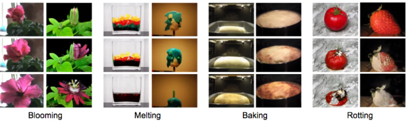
As a natural follow-up, in Chapter 3, we explore predicting the future states. Specifically, we utilize deep generative model to generate the depictions of the future state of objects (we train computational models to learn natural object transformations from videos). We explore several different generation tasks for modeling natural transformations. To enable the learning, we collect time-lapse videos demonstrating four different natural state transformations. Each transformation category includes one or multiple objects. The dataset contains 1463 high-quality time-lapse videos with alignment annotations from Amazon Mechanical Turk (AMT) and has been released publicly. The Figure 1.1 shows the example video frames of time-lapse videos from the dataset.
Figure 1.1: Example frames from our dataset of each transformation category: Blooming, Melting, Baking, and Rotting. In each column, time increases as you move down the column, showing how an object transforms.
Figure 1.2: We train a personalized model for a target individual in an Internet video. This model can synthesize the target person in novel poses (right) from the input frame (bottom left) driven by a different individual (top left).
we introduce a computational model to transfer any desired movement from a new reference video to the target person. We train this model only using several-minute-long video of the target person performing some random activities as Figure 1.2 shows. Compared with previous or concurrent works which investigate human pose transfer either under generalized settings (models trained across various individuals/scenes) or using single person lab-recorded videos. We we explore personalized motion transfer on videos obtained from the Internet, such as YouTube. Due to the more flexible property of Internet data (backgrounds are non-static or the range of poses demonstrated by the YouTuber are restricted), we break our task down into two sub tasks by proposing a two-stage framework to synthesis foreground human and backgrounds separately.
corresponded. The models are expected to learn associations between generated natural sound and visual inputs in the wild for various scenes and object interactions. Due to the missing of benchmark dataset for natural sound generation, we collect a large-scale video-audio dataset with visual and sound modalities closely related (the visual contents/objects are synchronized well with the according sound, e.g. when we hear dog barking sound, there should be dogs shown in the frames) to make the data ideal for the generation tasks. Our dataset is derived from AudioSet [Gemmeke et al., 2017] which is collected for audio event recognition but not ideal for visual to sound mapping task.
The contributes introduced by this dissertation include:
1. Define beyond-pixel mappings concept and formulate the problem through various aspects including temporal perception and future prediction, personalized motion transfer as well as mapping visual information to other modalities.
2. Propose two novel temporal prediction tasks in video domain: video pairwise ordering and future event prediction. Collect a new dataset of ego-centric videos of everyday life activities, including both individuals and families living in the same location.
3. Present a new problem of modeling natural object transformations with deep generative networks by utilizing time-lapse videos. A new dataset of 1463 time-lapse videos depicting 4 common object transformations has been collected.
4. Demonstrate personalized motion transfer on videos from the Internet. Propose a novel two-stage framework to synthesize people performing new movements and fuse them seamlessly with background scenes.
CHAPTER 2
Temporal Sequence Prediction
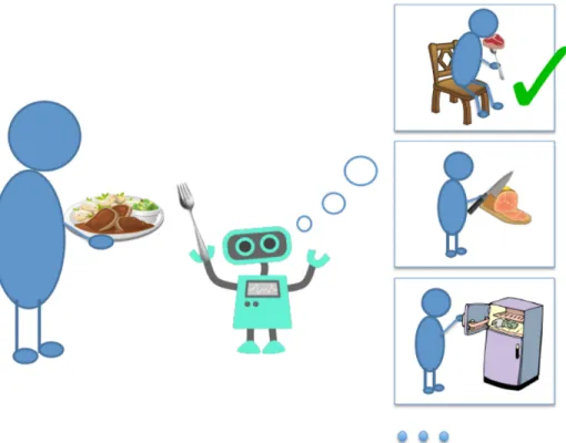
Given two video fragments of an single event, can we predict which moment usually happens first and next? Understanding the natural of temporal sequence of events is fundamental for future prediction. In this Chapter, we explore predicting temporal context beyond the frame, examining how well humans and computers can make predictions about what usually happens first and what will happen next during everyday activities. Such reasoning will be necessary for producing intelligent agents that can understand what a person is doing and anticipate what they are likely to do next. Both types of inference can help produce robots that more naturally interact with humans in our daily lives as Figure 2.1 shows.
We introduce two tasks related to temporal prediction. In the first task, given two short video snippets of an activity, the goal is to predict their correct temporal ordering. In the second task, given a longer context video plus two video snippets sampled from before or after the context video, the goal is to predict which video snippet was captured closest in time after the context video. These simplified task models the scenario of predicting the temporal sequence and future. The prediction has been applied on Ego-centric video domain (first person video), which has attracted increasing attention due to the rich information contained in egocentric visual data [Fathi et al., 2011a, Pirsiavash and Ramanan, 2012] and easier access to wearable recording devices as well as the potential as as a form of life-blogging [Lu and Grauman, 2013]. We collect a new dataset of ego-centric videos of everyday activities, which allows us to train both generalized and personalized temporal sequence prediction models.
Figure 2.1: If artificial intelligent agents could anticipate what will happen next under the everyday life activity scenarios, they are able to better interact with human.
[Zhou and Berg, 2015].
2.1 Temporal Prediction Tasks
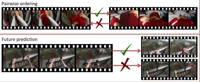
Figure 2.2: Illustration of our two temporal prediction tasks for ego-centric video of everyday activities. In the pairwise ordering task (above) the goal is to provide the correct temporal ordering for two short snippets of video from an activity. In the future prediction task (below), given a longer context video of an activity and two video snippets, the goal is to determine which snippet will occur (closest in time) after the context video.
raising it toward himself. Temporal predictions should tell us that the drinking action is more likely to occur (closest in time) after the context video than the other snippet.
These tasks have several advantages. They provide a measure of video understanding that is complementary to standard activity recognition with tasks that do not require semantic labels, but are easy to evaluate. They also provide quantitative measures for temporal prediction, one challenging aspect of general scene understanding. The tasks are also designed so that we can ask (multiple) people to perform the same tasks as the algorithms, allowing us to measure human performance on temporal prediction. In summary, this provides an initial first step toward enabling computers to understand the temporal nature of videos.
2.2 Dataset
while standing. All of these factors make for wide variation even in common everyday activities. While one insight is that although these factors, along with variations due to environment, may vary from person to person, a particular person might be quite consistent in how they perform each activity and in the locations in which they perform the activities. Therefore, along with building general temporal prediction models, we would also like to build models for prediction that can be personalized, either to a particular individual or to a particular environment. However, existing ego-centric dataset [Fathi et al., 2012a, Fathi et al., 2012b, Pirsiavash and Ramanan, 2012, Fathi et al., 2011b, Lee et al., 2012] designed for a variety of purposes, such as object recognition, activity recognition, social interaction detection and video summarization contain only one or a few examples of each activity performed by single subject. To enable this personalized learning, we have collected a dataset of first person videos of everyday activities, called the First Person Personalized Activities (FPPA) dataset, where each subject has performed every activity many times. We make use of this dataset for evaluating temporal prediction tasks, but it could also be used for general or personalized activity recognition.
2.2.1 Data collection
For data collection, we make use of a GoPro camera mounted on the user’s head using a head strap. The GoPro cameras record ego-centric data simulating the wearer’s viewpoint. Each camera captures a high-definition video at 1080p (1920x1080 resolution) with a wide field of view (133.6 degrees) at a rate of 30 frames per second.
We first provide each subject with a list of 5 daily activities (a list of activities is shown in Table 2.1. To encourage subjects to act naturally, they are not provided with any more details. Subjects are encouraged to film themselves completing each activity multiple times at different locations where they would normally perform them. Video recordings were captured in the subjects own homes or in public places (gym, lounge) that they usually visit. In total, our data is made up of 5 sets of videos. Two of the sets consist of videos from a single individual (single-subject) while 3 of the sets consist of videos from families, i.e. two or more people living together at the same location (family subject). We spread the data collection procedure of each set over two months to encourage
Activities Avg videos/subjects Avg locations/subjects Total videos/locations Wash hands 24.2 (19-34) 3.2 (2-7) 121 / 16 Put on shoes 22.8 (21-29) 3.0 (2-6) 114 / 15 Use fridge 26.4 (21-31) 1.6 (1-3) 132 / 8 Drink water 23.2 (16-31) 3.6 (2-7) 116 / 18 Put on clothes 21.6 (16-26) 3.4 (2-5) 108 / 17
Table 2.1: Statistics of FPPA dataset including averaged number of videos from per subject (col2), averaged number of locations per subjects (col 3) and total number of videos and locations (col3). The contents in brackets show the minimal to maximal numbers. The total number of video clips in the dataset is 591.
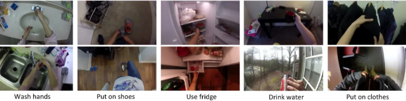
Figure 2.3: Example frames of 5 activities from our dataset. People perform everyday activities in various locations, and according to their own preferences, e.g. when putting on shoes people might squat down or stand or use a chair.
2.2.2 Characteristics and statistics
The main characteristic of the FPPA dataset is that it is built to enable learning both general and personalized models for temporal prediction. As such we collect a large number of examples of each activity from each subject and for each location. Table 2.1 shows statistics of our dataset, including the per subject average number of the video clips for each activity, and the average number of locations in which each subject performed the activity. On average subjects have performed each activity approximately 20 times. As habits vary from subject to subject, some subjects have performed an activity in a single location while others have performed them in up to 7 different locations. Figure 2.3 shows some example frames from activities performed by different subjects. 2.3 Human experiments
and what specific implementation features should be used for the task, e.g. what length snippets should we use, or how far separated in time should the snippets be so that they are still temporally distinguishable? Therefore, we design two human experiments to gain some useful insights into the pairwise ordering task and then configure our pairwise ordering and future prediction tasks based on these analyses.
2.3.1 Snippet size
We design an experiment to evaluate the effect of snippet length on human perceptions of pairwise ordering using Amazon Mechanical Turk (AMT) as our crowdsourcing platform. For each activity we randomly pick 100 pairs of snippets from videos of the activity, where the central frame for each snippet is selected at a random temporal position within the video. We vary snippet size as 1, 10, 30, 60, or 100 frames (snippet size 1 is a static image). For each pair of snippets we ask 3 AMT workers to tell us which snippet should come first in temporal ordering. To limit bias, we randomly reshuffle the left-right placement of snippets in our Turk interface, and only allow workers to see one snippet length for a particular pair of snippets.
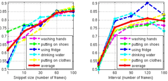
Figure 2.4 (left) shows the effect of snippet size on human performance. One interesting observation is that for the "using fridge" and "drinking water" activities there is an obvious increase in human performance between a snippet size of 1 (static image) and snippet size of 10 frames. One reason for this could be that these activities are relatively symmetric so it may be difficult to tell from a single frame whether the person is opening or closing the fridge, or picking up or putting down a cup. For a video snippet, motion cues help people resolve these ambiguities.
Based on these experiments, we find that human performance for pairwise ordering increases greatly past single frame snippets, but then levels off at about 60 frames. For length 60 frame snippets we find that average performance across users is about 80 to 85% for all activities. Therefore, for the rest of our human and computer experiments we use a snippet length of 60 frames.
2.3.2 Snippet interval
Figure 2.4: Human performance on pairwise ordering. Left shows performance as snippet size varies. Right shows performance as interval varies.
between center frames of 1, 60, 90, 120, or 180 frames. We limit Turker bias in the same manner as the previous experiment.
The results of this experiment are shown in Figure 2.3 (right). Agreeing with intuition, when the temporal offset between two snippets is extremely small (e.g., 1 frame), it is difficult for people to predict the correct pairwise ordering between snippets. As the interval between snippets increases, human performance also increases, but then levels off or even drops as the interval between the snippets gets very long (e.g., 180 frames). For activities such as "putting on clothes" which have clear steps in a relatively lengthy procedure, larger intervals tend to increase performance. For activities like drinking water, the accuracy initially rises with larger intervals then decreases for longer intervals. There are several potential reasons for this: (1) the most distinctive parts of the procedure may be very short, or (2) this activity is periodic (people may repeat the sipping portion of the action multiple times in one drinking activity). Both reasons can cause ambiguity for longer intervals.
2.4 Approaches
2.4.1 Video snippet representation
of the wearer [Aghazadeh et al., 2011]. Quite a few previous works have used techniques such as, hand detection, object detection, or motion features such as optical flow to represent ego-centric videos [Fathi et al., 2011a, Fathi et al., 2012a, Kitani et al., 2011, Pirsiavash and Ramanan, 2012, Ryoo and Matthies, 2013], but how to represent first person videos effectively for temporal prediction tasks is an open question. Recently the use of features learned by deep networks have achieved success in many different vision tasks such as object recognition and detection [Donahue et al., 2013, Girshick et al., 2014], or activity recognition [Simonyan and Zisserman, 2014a]. In this work, we represent video snippets using learned deep features for objects, scenes, and motion.
Object representation: For each frame of a video snippet, we extract the 4096 dimension fc6 layer of the VGG model [Simonyan and Zisserman, 2014b], pre-trained to recognize 1000 Ima-geNet [Deng et al., 2009] object categories. Then we apply max-pooling over a 10-frame window around the frame to implicitly capture some temporal information about objects within the snippet.
Scene representation: For each frame of a video snippet, to model scene/environment in-formation for video snippets, we extract the 4096 dimension fc7 layer of the Caffe reference model [Jia et al., 2014], pre-trained on the scene-centric Places dataset [Zhou et al., 2014]. Again, we apply max-pooling in a 10-frame window to capture temporal scene information.
Motion representation: Inspired by recent work on deep networks for activity recognition, we re-implement the Temporal Convnet approach of [Simonyan and Zisserman, 2014a]. Their method takes a two stream approach to activity recognition using both object and optical flow features. Our reimplementation of their method achieves an accuracy of 78% on the UCF-101 dataset compared to their reported result of 81%. From the optical flow portion of the Temporal Convnet, we extract the 4096 dimensional fc6 layer as our motion representation.
2.4.2 Pairwise prediction methods
We evaluate several methods for predicting pairwise temporal ordering. The first two are nearest neighbor based methods. The intuition behind these methods is that if two video snippets have similar appearance and motion then we can directly transfer temporal information from one video to the other. One challenge for nearest neighbor methods is that activities can be completed at different rates, therefore we experiment with temporal warping methods to align video snippets. Next we present a regression method that tries to directly predict the time of a video snippet. All three of these models attempt to estimate when a video snippet occurred within a larger activity. Given two snippets we can then predict their pairwise ordering based on their relative estimated times. Our final two methods are trained to directly predict pairwise ordering. Given two video snippets, A and B, we train an SVM and a fully-connected network to predict whether or not snippet A occurred temporally before B. For all of these methods we assume that we know what activity is occurring to focus our efforts on the task of temporal prediction. These methods could be incorporated into a broader system to estimate both activity recognition and temporal predictions.
NN Frac: We first represent the temporal information of all snippets as a real value computed as the temporal position of the snippet relative to the length of the entire action. For each query snippet, using one or more of our feature representations, we retrieve its nearest neighbor snippet from the training set and transfer the nearest neighbor’s relative time to the query. Similarity is measured as cosine similarity.
NN DTW: We perform nearest neighbor prediction as before, but a priori first align all training videos for an activity temporally using Dynamic Time Warping (DWT) [Sakoe and Chiba, 1978]. DWT is a dynamic programming algorithm that keeps track of the cost of the best path of the alignment. Here the cost function is defined as the Euclidean distance between each pair of video snippets.
SVM: We train a linear SVM model directly for the pairwise prediction task. Input to the model are concatenated features from a pair of snippets, A and B. Output of the model is a binary prediction ∈ {1,−1} where the model predicts 1 to indicate that A temporally occurs before B and -1 to indicate that A occurs after B. To train this model, we randomly sample pairs of snippets from activities with intervals between the snippets ranging from 60 to 300 frames. The learning parameter is set using cross-validation.
FcNet: Inspired by the metric network architecture introduced in [Han et al., 2015], we train a three layer fully-connected network to predict pairwise ordering. The scenario is the same as the SVM method, that is, we model the task as a binary classification problem. The first two layers of this network have 512 units and use Rectified Linear Unit (ReLU) as the non-linear activation function. The last layer has 2 output units, estimating the probability that snippet A occurs before or after B. During training we apply mini-batch gradient decent and cross-entropy loss. We set the learning rate to be 0.001, dropout rate 0.5, momentum 0.9, and train for 30000 iterations. The hyper-parameters are decided using a validation set.
2.5 Experiments
2.5.1 General pairwise ordering prediction
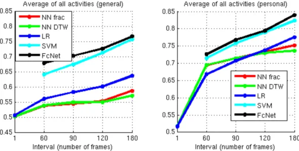
Figure 2.5: Model performance on pairwise ordering. Left shows prediction performance of general models (trained on other subjects). Right shows personalized model performance (trained on other videos from the same subject).
Methods Washing hands Putting on shoes Using fridge Drinking water Putting on clothes Average
NN frac(O) 0.5707 0.5257 0.5494 0.5459 0.5604 0.5504
NN frac(OS) 0.5879 0.5402 0.5468 0.5432 0.5421 0.5521
NN frac(OSM) 0.5694 0.5299 0.5884 0.4938 0.5807 0.5525
NN DTW(O) 0.5835 0.5302 0.5400 0.4709 0.5501 0.5350
NN DTW(OS) 0.5610 0.5447 0.5387 0.5335 0.5533 0.5462
NN DTW(OSM) 0.5738 0.5257 0.5884 0.4855 0.5758 0.5499
LR(O) 0.5635 0.5502 0.6296 0.5844 0.6034 0.5862
LR(OS) 0.5550 0.5853 0.6233 0.5732 0.5923 0.5858
LR(OSM) 0.5536 0.5964 0.6583 0.6039 0.5950 0.6014
SVM(O) 0.6392 0.7026 0.7351 0.6848 0.6967 0.6917
SVM(OS) 0.6609 0.7270 0.7435 0.6845 0.7044 0.7041
SVM(OSM) 0.6749 0.6945 0.7402 0.7538 0.7006 0.7128
2.5.2 Personalized pairwise ordering prediction
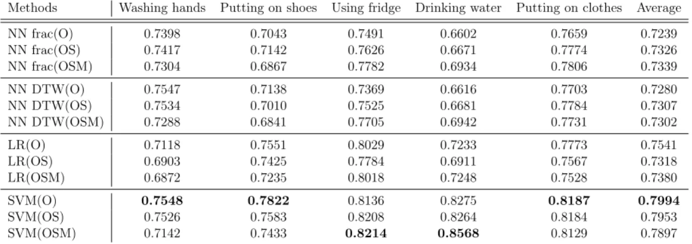
We evaluate two types of personalized models: models personalized to a particular subject or to a particular location. First, we evaluate personalization where we use different video clips from a single subject for training and testing by applying the leave-one-out method. Since the amount of personalized data is quite limited, for the FcNet, to prevent overfitting, we fine-tune the general network using personalized data for another 25000 iterations (the hyper-parameters remain unchanged). Figure 2.5 (right) shows averaged results across activity, subject, and interval for models personalized to a subject. In these experiments, we see improved performance on the pairwise ordering task compared to general prediction models trained on other subjects, indicating that the personalized models are able to better adapt to a particular individual’s habits and daily environments. Table 2.3 shows personalized pairwise ordering accuracy for each activity type and feature combination for interval size of 120. Unlike the general prediction model, the models achieve best performance with the object representation based model, but for some activities incorporating additional features is helpful. We provide several more experiments to further understand personalization. To evaluate generalization for individuals between locations, we train models for the single subjects with different locations in training vs testing. To evaluate generalization between people in the same location, we train models for family-subjects with different family members in training vs. testing. And we also evaluate the effect of training set size. Due to the limited data, for each experiment we apply the SVM method on object, scene, and motion features (Figure 2.6 shows quantitative results). For the individual and location experiments, accuracies are still reasonable compared to the previous personalization experiment. For the training size experiment, we find that the amount of training data required for accurate prediction varies, with some activities benefiting from larger training sizes (e.g. "using fridge") and others achieving surprisingly good accuracy with only 5 samples (e.g. "putting on clothes").
Methods Washing hands Putting on shoes Using fridge Drinking water Putting on clothes Average
NN frac(O) 0.7398 0.7043 0.7491 0.6602 0.7659 0.7239
NN frac(OS) 0.7417 0.7142 0.7626 0.6671 0.7774 0.7326
NN frac(OSM) 0.7304 0.6867 0.7782 0.6934 0.7806 0.7339
NN DTW(O) 0.7547 0.7138 0.7369 0.6616 0.7703 0.7280
NN DTW(OS) 0.7534 0.7010 0.7525 0.6681 0.7784 0.7307
NN DTW(OSM) 0.7288 0.6841 0.7705 0.6942 0.7731 0.7302
LR(O) 0.7118 0.7551 0.8029 0.7233 0.7773 0.7541
LR(OS) 0.6903 0.7425 0.7784 0.6911 0.7567 0.7318
LR(OSM) 0.6872 0.7235 0.8018 0.7248 0.7528 0.7380
SVM(O) 0.7548 0.7822 0.8136 0.8275 0.8187 0.7994
SVM(OS) 0.7526 0.7583 0.8208 0.8264 0.8184 0.7953
SVM(OSM) 0.7142 0.7433 0.8214 0.8568 0.8129 0.7897
Table 2.3: Accuracy of pairwise temporal ordering using personalized prediction models (trained and tested on different videos from the same subject) for interval size 120. Here O indicates object features, S scene features, and M motion features
Figure 2.7: Inferring temporal information for an entire video sequence. Colorbar indicates the reordering of original time information (black=start, white=end).
2.5.3 Future prediction task
Next we design the future prediction task where we are provided with a 3 second context video, C, of an activity and two video snippets, A and B, and we are asked to predict which will occur (soonest in time) after C. A is sampled from soon after the context video (randomly selected, but no more than 3 seconds in the future) and B is randomly sampled, either from further in the future or from the time period prior to C. A correct prediction will predict snippet A as happening next.
Computer prediction: Given an algorithm to predict pairwise orderings between snippets, it is straightforward to extend this algorithm to the future prediction task. We compute all pairwise orderings between A, B, and C, and then select the snippet that is most likely to follow after C in temporal order. For these experiments we use combined object, scene, and motion features (Figure 2.8 shows examples).
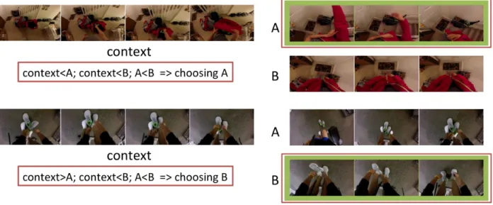
Figure 2.8: Visualization results of computer-based future prediction. Text within red borders are the pairwise ordering results generated by our method. Right shows algorithm proposed future prediction (red border) and ground truth (green border).
Activities LRg LRp SVMg SVMp Human Wash hands 0.5750 0.7050 0.6350 0.7550 0.7816 Put on shoes 0.5700 0.7500 0.7000 0.7250 0.8733 Use fridge 0.6250 0.6800 0.6100 0.7100 0.9284 Drink water 0.5850 0.6700 0.6500 0.7300 0.8717 Put on clothes 0.6350 0.7950 0.7100 0.8350 0.8866 Average 0.5980 0.7200 0.6630 0.7510 0.8686
Figure 2.9: Left is the pairwise ordering accuracy of subset of UCF101 dataset. Note that video clips in UCF101 are very short for some actions, the largest interval is only 90. Right is the forward/backward classification accuracy of our method and Flow-Words method in [Pickup et al., 2014b] testing on our dataset
two video snippets and ask the worker to identify which will follow soonest in time after the video. Table 2.4 shows accuracies of human and computer predictions. Personalized models outperform the general models significantly, achieving an average accuracy of 75%. Human performance on this task is also quite good (87%). We also want to understand how well algorithms can perform on the future prediction given snippets from two different videos. Here we first ask humans to perform the future prediction task and then select data with high inter-subject agreement. On this data, using the human predictions as ground truth, the general SVM and FcNet models achieve 66.22% and 66.99% accuracy respectively.
2.5.4 Additional experiments
Pairwise ordering on UCF101: For comparison, we also evaluate our pairwise ordering task on a subset of a wildly used third person action recognition dataset, UCF101. We select 10 categories of action with reasonably long duration and non-repetitive movements. Each category contains more than 100 video clips. In this experiment we evaluate our SVM method and keep other settings (snippet size, feature) the same as our previous experiments. We run 3 train/test splits provided by the UCF official project webpage. Figure 2.9 (left) shows performance. We see that for third person activity videos, our method can achieve even better performance than for first person videos.
forward or backward. We implement their FlowWords classification method which is based on a SIFT-like descriptor and linear SVM. For specific information and parameter settings, please refer to their work. Predicting the temporal direction of video clips can be solved by our pairwise ordering predictions. Our method achieves comparable performance on this task. For each testing video clip, we sample all its snippet pairs with interval 90 and 120 along the video and apply our general SVM model to classify the ordering, then we do majority vote to decide the flow direction of the video. Figure 2.9 (right) shows the average accuracy for Flow-Words and our method.
2.6 Conclusions
CHAPTER 3
Future object state prediction
Based on life-long observations of physical, chemical, and biologic phenomena in the natural world, humans can often easily picture in their minds what an object will look like in the future. But, what about computers? In this paper we seek to learn computational models of how the world works through observation. In particular, we explore the use of generative models to create depictions of objects at future times. To enable this learning, we collect time-lapse videos demonstrating four different natural state transformations: melting, blooming, baking, and rotting. Several of these transformations are applicable to a variety of objects. We train models for each transformation - irrespective of the object undergoing the transformation - under the assumption that these transformations have shared underlying physical properties that can be learned. Future prediction has been explored in previous works for generating the next frame or next few frames of a video [Srivastava et al., 2015, Mathieu et al., 2015, Ranzato et al., 2014]. Our focus, in comparison, is to model general natural object transformations and to model future prediction at a longer time scale (minutes to days) than previous approaches.
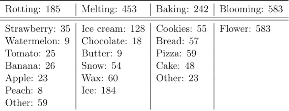
Rotting: 185 Melting: 453 Baking: 242 Blooming: 583 Strawberry: 35 Ice cream: 128 Cookies: 55 Flower: 583 Watermelon: 9 Chocolate: 18 Bread: 57
Tomato: 25 Butter: 9 Pizza: 59 Banana: 26 Snow: 54 Cake: 48 Apple: 23 Wax: 60 Other: 23 Peach: 8 Ice: 184
Other: 59
Table 3.1: Statistics of our transformation categories. Some categories contain multiple objects (e.g. ice cream, chocolate, etc melting) while others apply only to a specific object (e.g. flowers blooming). Values indicate the total number of videos collected for each category.
t+2m). These models are trained on images with varying time gaps. In our last prediction task, our goal is to recursively generate the future states of an object given a single input image of the object. For this task, we use a recurrent neural network to recursively generate future depictions. For each of the described future generation tasks, we also explore the effectiveness of pre-training on a large set of images, followed by fine-tuning on time-lapse data for improving performance.
We first describe the time-lapse dataset and the data collection in Section 3.1. In Section 3.2, we discuss three future generation tasks we mentioned above and the training approaches. Finally, we provide both qualitative and quantitative evaluation results as well as the human experiments in Section 3.3.
3.1 Time-lapse video dataset
Given the high-level goal of understanding temporal transformations of objects, we require a collection of videos showing temporal state changes. Therefore, we collect a large set of object-centric timelapse videos from the web. Timelapse videos are ideal for our purposes since they are designed to show an entire transformation (or a portion of a transformation) within a short period of time. 3.1.1 Data collection
results in a dataset of more than 5000 videos. This dataset could be extended to a wider variety of transformations or to more complex multi-object transformations, but as a first step we focus on these 4 as our initial goal set of transformations for learning.
For ease of learning, ideally these videos should be object-centric with a static camera capturing an entire object transformation. However, many videos in the initial data collection stage do not meet these requirements. Therefore, we clean the data using AMT as a crowdsourcing platform. Each video is examined by 3 Turkers who are asked questions related to video quality. Videos that are not timelapse, contain severe camera motion or are not consistent with the query labels are removed. We also manually adjust parts of the videos which are playing backwards (a technique used in some time-lapse videos), contain more than one round of the specified transformation, and remove irrelevant prolog/epilog. Finally our resulting dataset contains 1463 high quality object based timelapse videos. Table 3.1 shows the statistics of transformation categories and their respective object counts. Figure 1.1 (Section 1.2) shows example frames of each transformation category. 3.1.2 Transformation degree annotation
To learn natural transformation models of objects from videos, we need to first label the degree of transformation throughout the videos. In language, people use text labels to describe different states, for instance, fresh vs rotted apple. However, the transformation from one state to another is really a continuous evolution. Therefore, we represent the degree of transformation with a real number, assigning the start state a value of 0 (not at all rotten) and the end state (completely rotten) a value of 1. To annotate objects from different videos we could naively assign the first frame a value of 0 and the last frame a value of 1, interpolating in between. However, we observe that some time-lapse videos may not depict entire transformations, resulting in poor alignments.
Figure 3.1: Model architectures of three generation tasks: (a) Pairwise generator; (b) Two stack generator; (c) Recurrent generator.
displayed video does not depict an entire transformation, Turkers may align less than 5 frames with the reference. Each target video is aligned by 3 Turkers and the median of their responses is used as annotation labels(linearly interpolating degrees between labeled target frames). This provides us with consistent annotations of transformation degree between videos.
3.2 Future state generation
Our goal is to generate depictions of the future state of objects. In this work, we explore frameworks for 3 temporal prediction tasks. In the first task (Section 3.2.1), called pairwise generation, we input an object-centric frame and the model generates an image showing the future state of this object. Here the degree of the future state transformation - how far in the future we want the depiction to show - is controlled by a conditional term in the model. In the second task (Section 3.2.2) we have two inputs to the model: two frames from the same video showing a state transformation at two points in time. The goal of this model is to generate a third image that continues the trend of the transformation depicted by the first and second input. We call this "two stack" generation. In the third task (Section 3.2.3), called "recurrent generation", the input is a single frame and the goal is to recursively generate images that exhibit future degrees of the transformation in a recurrent model framework.
3.2.1 Pairwise generation
Figure 3.1(a), where the input and output size are 64x64 with 3 channels and encoding and decoding parts are symmetric. Both encoding and decoding parts consists of 4 convolution/deconvolution layers with the kernel size 5x5 and a stride of 2, meaning that at each layer the height and width of the output feature map decreases/increases by a factor of 2 with 64, 128, 256, 512/512, 256, 128, 64 channels respectively. Each conv/deconv layer, except the last layer, is followed by a batch normalization operation [Ioffe and Szegedy, 2015] and ReLU activation function [Nair and Hinton, 2010]. For the last layer we use Tanh as the activation function. The size of the hidden variable z (center) is 512. We represent the conditional term encoding the degree of elapsed time between the input and output as a 4 dimensional one-hot vector, representing 4 possible degrees. This is connected with a linear layer (512) and concatenated with z to adjust the degree of the future depiction. Below we describe experiments with different loss functions and training approaches for this network.
p_mse: As a baseline, we use pixel-wised mean square error(p_mse) between prediction output and ground truth as the loss function. Previous image generation works [Srivastava et al., 2015, Mathieu et al., 2015, Ranzato et al., 2014, Pathak et al., 2016] postulate that pixel-wisedl2criterion is one cause of output generation blurriness. We also observe this effect in the outputs produced by this baseline model.
architecture of D is the same as the encoder of G, except that the last output is a scalar and connect with sigmoid function. D also incorporates the conditional term by connecting a one-hot vector with a linear layer and reshaping to the same size as the input image then concatenating in the third dimension. The output of D is a probability, which will be large if the input is a real image and small if the input is a generated image. For this framework, the loss is formulated as a combination of the MSE and adversarial loss:
LG=Lp_mse+λadv∗Ladv (3.1)
where Lp_mse is the mean square error loss, wherexis the input image, c is the conditional term, G(.) is the output of the generation model, andyis the ground truth future image at time = current time +c.
Lp_mse=|y−G(x, c)|2 (3.2)
And, Ladv is a binary cross-entropy loss withα = 1 that penalizes if the generated image does not look like a real image. D[.] is the scalar probability output by the discriminator.
Ladv =−αlog(D[G(x, c), c])−(1−α) log(1−D[G(x, c), c]) (3.3)
During training, the binary cross-entropy loss is used to train D on both real and generated images. For details of jointly training adversarial structures, please refer to [Goodfellow et al., 2014].
p_g_mse+adv: Inspired by [Mathieu et al., 2015], where they introduce gradient basedl1 orl2 loss to sharpen generated images. We also evaluate a loss function that is a combination of pixel-wise MSE, gradient based MSE, and adversarial loss:
LG =Lp_mse+Lg_mse+λadv∗Ladv (3.4)
whereLg_mse represents mean square error in the gradient domain defined as:
gx[.]andgy[.]are the gradient operations along the x and y axis of images. We could apply different weights to Lp_mse andLg_mse, but in this work we simply weight them equally.
p_g_mse+adv+ft: Since we have limited training data for each transformation, we investigate the use of pre-training for improving generation quality. In this method we use the same loss function as the last method, but instead of training the adversarial network from scratch, training proceeds in two stages. The first stage is a reconstruction stage where we train the generation model using random static images for the reconstruction task. Here the goal is for the output image to match the input image as well as possible even though passing through a bottleneck during generation. In the second stage, the fine-tuning stage, we fine-tune the network for the temporal generation task using our timelapse data. By first pre-training for the reconstruction task, we expect the network to obtain a good initialization, capturing a representation that will be useful for kick-starting the temporal generation fine-tuning.
3.2.2 Two stack generation
In this scenario, we want to generate an image that shows the future state of an object given two input images showing the object in two stages of its transformation. The output should continue the transformation pattern demonstrated in the input images, i.e. if the input images depict the object at time t and t+m, then the output should depict the object at time t+2m. We design the generation model using two stacks in the encoding part of the model as shown in Fig. 3.1(b). The structures of the two stacks are the same and are also identical to the encoding part of the pairwise generation model. The hidden variablesz1 andz2 are both 512 dimensions, and are concatenated together and fed into the decoding part, which is also the same as the previous pairwise generation model. The two stacks are sequential, trained independently without shared weights.
3.2.3 Recurrent generation
In this scenario, we would like to recursively generate future images of an object given only a single image of its current temporal state. In particular, we use a recurrent neural network framework for generation where each time step generates an image of the object at a fixed degree interval in the future. This model structure is shown in Fig. 3.1(c). After hidden variable z, we add a LSTM[Hochreiter and Schmidhuber, 1997] layer. For each time step, the LSTM layer takes both
z and the output from the previous time step as inputs and sends a 512 dimension vector to the decoder. The structure of the encoder and decoder are the same as in the previous scenarios, where the decoding portions for each time slot share the same weights.
We evaluate three loss functions in this network: p_mse+adv, p_g_mse+adv as well as p_g_mse+adv+ft. The structure of the discriminator is again the same without the conditional term (as in the two-stack model). For fine-tuning, during reconstruction training, we train the model to recurrently output the same static image as the input at each time step.
3.3 Experiments
In this section, we discuss the training process and parameter settings for all experiments (Sec 3.3.1). Then, we describe dataset pre-processing and augmentation (Sec 3.3.2). Finally, we discuss quantitative and qualitative analysis of results for: pairwise generation (Sec 3.3.3), two-stack generation (Sec 3.3.4), and recurrent generation (Sec 3.3.5) as well as the human experiments and the visualization results (Sec 3.3.6).
3.3.1 Training and parameter settings
Unless otherwise specified training and parameter setting details are applied to all models. During training, we apply Adam Stochastic Optimization[Kingma and Ba, 2014] with learning rate 0.0002 and minibatch of size 64. In the loss functions where we combine mean square error loss with adversarial loss (as in equation 3.1), we set the weight of the adversarial loss to λadv = 0.2 for all experiments.
3.3.2 Dataset preprocessing and augmentation
testing sets in a ratio of 0.85 : 0.15. Then, we sample frame pairs (for pairwise generation) or groups of frames (for two-stack and recurrent generation) from the training and testing videos. Frames are resized to 64x64 for generation. To prevent overfitting, we also perform data augmentation training pairs or groups by incorporating frame crops and left-right flipping.
Reconstruction dataset: This dataset contains static images used to pre-train our models on reconstruction tasks. Initially, we tried training only on objects depicted in the timelapse videos and observed performance improvement. However, collecting images of specific object categories is a tedious task at large-scale. Therefore, we also tried pre-training on random images (scene images or images of random objects) and found that the results were competitive. This implies that the content of the images is not as important as encouraging the networks to learn how to reconstruct arbitrary input images well. We randomly download 50101 images from ImageNet[Deng et al., 2009] as our reconstruction dataset. The advantage of this strategy is that we are able to use the same group of images for every transformation model and task.
3.3.3 Pairwise generation results
In the pairwise generation task, we input an image of an object and the model outputs depiction of the future state of the object, where the degree of transformation is controlled by a conditional term. The conditional term is a 4 dimensional one-hot vector which indicates whether the predicted output should be 0, 0.25, 0.5 or 0.75 degrees in the future from the input frame. We sample frame pairs from timelapse videos based on annotated degree value intervals. A 0 degree interval means that the input and output training images are identical. We consider 0 degree pairs as auxiliary pairs, useful for two reasons: 1) They help augment the training data with video frames (which display different properties from still images), and 2) The prediction quality of image reconstruction is highly correlated with the quality of future generation. Pairs from 0 degree transformations can be easily be evaluated in terms of reconstruction quality since the prediction should ideally exactly match the ground truth image. Predictions for future degree transformations are somewhat more subjective. For example, from a bud the resulting generated bloom may look like a perfectly valid flower, but may not match the exact flower shape that this particular bud grew into (an example is shown in Figure. 3.2 row 1).
Figure 3.2: Pairwise generation results for: Blooming (rows 1-3), Melting (rows 4-5), Baking (rows 6-7) and Rotting (rows 8-9). Input(a), p_mse(b), p_mse+adv(c), p_g_mse+adv(d), p_g_mse+adv+ft(e), Ground truth frames(f). Black frames in the ground truth indicate video did not depict transformation that far in the future.
Pairwise Two stack Recurrent
PSNR SSIM MSE PSNR SSIM MSE PSNR SSIM MSE
p_mse+adv 17.0409 0.5576 0.0227 17.7425 0.5970 0.0185 17.2758 0.5747 0.0211 p_g_mse+adv 17.0660 0.5720 0.0224 17.9157 0.6122 0.0177 17.2951 0.5749 0.0214 p_g_mse+adv+ft 17.4784 0.6036 0.0207 18.6812 0.6566 0.0153 18.3357 0.6283 0.0166
Table 3.2: Quantitative evaluation of: Pairwise generation, Two stack generation, and Recurrent tasks. For PSNR and SSIM larger is better, while for MSE lower is better.
Figure 3.3: Two stack generation results for Blooming (a), Melting (b), Baking (c) and Rotting (d). For each we show the two input frames (col 1-2), and results for: p_mse+adv (col 3), p_g_mse+adv (col 4), p_g_mse+adv+ft (col 5) and ground truth (col 6)
3.3.4 Two stack generation results
Figure 3.4: Two stack generation with varying time between input images. For each example we show: the two input images (col 1-2), p_mse+adv (col 3), p_g_mse+adv (col 4), p_g_mse+adv+ft (col 5) and ground truth (col 6). The models are able to vary their outputs depending on elapsed
time between inputs.
Pairwise Two stack Recurrent
BL ADV Grad Ft ADV Grad Ft ADV Grad Ft
Blooming 0.1320 0.2300 0.2880 0.3500 0.3080 0.3240 0.3680 0.3320 0.2860 0.3820 Melting 0.1680 0.2520 0.2760 0.3040 0.3400 0.3120 0.3480 0.3180 0.3220 0.3600 Baking 0.1620 0.2600 0.2840 0.2940 0.3120 0.3200 0.3680 0.2780 0.3540 0.3680 Rotting 0.1340 0.2020 0.2580 0.4060 0.3040 0.2640 0.4320 0.2940 0.2900 0.4160 Average 0.1490 0.2360 0.2765 0.3385 0.3160 0.3050 0.3790 0.3055 0.3130 0.3815
Table 3.3: Human evaluation results: BL stands for p_mse method, ADV (p_mse+adv), Grad(p_g_mse+adv) and Ft(p_g_mse+adv+ft)
but also learn to generate the correct time interval based on the input images. Figure. 3.4 shows input images with different amounts of elapsed time. We can see that the models are able to vary how far in the future to generate based on the input image interval.
3.3.5 Recurrent generation results
For our recurrent generation task, we want to train a model to generate multiple future states of an object given a single input frame. Due to limited data we recursively generate 4 time steps. During training, we sample groups of frames from timelapse videos. Each group contains 5 frames, the first being the input, and the rests having 0, 0.1, 0.2, 0.3 degree intervals from the input. As in the previous tasks, the reconstruction outputs are used for quantitative evaluation.
3.3.6 Additional experiments
Human Evaluations: As previously described, object future state prediction is sometimes not well defined. Many different possible futures may be considered reasonable to a human observer. Therefore, we design human experiments to judge the quality of our generated future states. For each transformation category and generation task, we randomly pick 500 test cases. Human subjects are shown one (or two for two stack generation) input image and future images generated by each method (randomly sorted to avoid biases in human selection). Subjects are asked to choose the image that most reasonably shows the future object state.
Results are shown in Table 3.3, where numbers indicate the fraction of cases where humans selected results from each method as the best future prediction. For pairwise generation (cols 2-5), the p_g_mse+adv+ftmethod achieves the most human preferences, while the baseline performs worst by a large margin. For both two stack generation (cols 6-8) and recurrent generation (cols 9-11), p_mse+adv andp_g_mse+advare competitive, but again making use of pre-training plus fine-tuning obtains largest number of human preferences.
Image retrieval: We also add a simple retrieval experiment on Pairwise generation results using pixelwise similarity. We count retrievals within reasonable distance (20% of video length) to the ground truth as correct, achieving average accuracies on top-1/5 of p_mse+adv:0.68/0.94; p_g_mse+adv: 0.72/0.95; and p_g_mse+adv+ft: 0.90/0.98.
Visualizations: Object state transformations often lead to physical changes in the shape of an object. To further understand what our models have learned, we provide some simple visualizations of motion features computed on generated images. Visualizations are computed on results of the p_g_mse+adv+ft recurrent model since we want to show the temporal trends of the learned transformations. For each testing case, we compute 3 optical flow maps in the x and y directions between the input image and the second, third, and fourth generated images. We cluster each using kmeans (k=4). Then, for each cluster, we average the optical flow maps in the x and y directions.
Figure 3.6: Visualization results of learned transformations: x axis flows of blooming (a), y axis flows of melting (b), y axis flows of baking (c) and y axis flows of rotting (d)
baking, consistent with the object inflating up and down. For rotting (d), we observe that the upper part of the object inflates with mold or shrinks due to dehydration.
3.4 Conclusions
CHAPTER 4
Personalized motion transfer
In this chapter, we develop computational methods for imitating human movements. In par-ticular, we train a model using one several-minute-long video of a target person and can then transfer any desired movement from a new reference video to the target person (maintaining ap-pearance) as Figure 1.2 (Section 1.2) shows. Previous work [Ma et al., 2017, Siarohin et al., 2018, Balakrishnan et al., 2018, Chan et al., 2018] investigates human pose transfer either under general-ized settings (models trained across various individuals/scenes) or using single person lab-recorded videos. In this work, we explore personalized motion transfer on videos obtained from the Internet, such as YouTube. With such data pre-recorded in uncontrolled ways, our models are required to generalize well to novel poses, as we cannot ask a person on YouTube to demonstrate the entire range of poses we might want to generate. We show example frames of the Internet videos used as training data in Figure 4.1.
Figure 4.1: Example frames of personal videos from YouTube (from left to right are: Video_01 to Video_08).
results, we also apply temporal smoothing to generate temporally coherent movements and use hand, foot, and face landmarks to enhance local body details. We describe our method in Section 4.1. To evaluate the effectiveness of the proposed method, we conduct both numerical evaluations and human experiments on generated results in Section 4.2.
4.1 Approach
We formulate the personalized motion transfer task as follows. Given an input frame Iin and a reference frameIref of sizeH×W, as well as their associated human poses Pin and Pref, we would like to learn a mappingF that generates an output frameIout with the reference pose transferred to the target person in the input frame:
Iout=F(Iin, Pin, Pref) (4.1)
where Iout retains the same human appearance and background scene asIin while rendering with the reference pose,Pref. During training, we sample random frame pairs from a personal video as our training data(Iin, Iref).
We treat the human body part segments from Iin as tangram pieces1 which are placed on a composition image according to the layout of reference pose, Pref. A similar step is used in [Balakrishnan et al., 2018]. This provides us with a good initial image on top of which we apply the human synthesis part of our method. The body part transform process is illustrated in Fig. 4.2 and
Figure 4.2: Body parts transformation. STN aligns the body parts of Iin with target pose Pref, producing body segments represented as a 3D volume T.
described in detail in Section 4.1.1.
Figure 4.3 shows the architecture of our two-stage model. The human synthesis stage (a) takes the transformed body parts as input and produces a foreground body image, filling the “holes” between transformed segments and adjusting details (e.g., angle of face) to produce a photo-realistic image of the target person in the reference pose (Section 4.1.3). In the second stage, a fusion network (b) takes the generated foreground and a fixed background image as inputs and generates the final synthesized outputIout (Section 4.1.4). The fusion network combines the foreground and background, fixing discontinuous foreground boundaries and adding important details such as shadows. We design special training techniques and loss functions as discussed in Section 4.1.5.
4.1.1 Human body part transformation
For each frame pair(Iin, Iref), we first apply a human body parsing algorithm [Fang et al., 2018] onIin as illustrated in Fig. 4.2, where Hin is the human parsing map and ⊗represents element-wise multiplication. The person from the input frame is segmented into 10 body parts (head, torso, left/right upper arms, left/right lower arms, left/right upper legs, left/right lower legs). We also employ the AlphaPose [Fang et al., 2017] pose estimation algorithm to detect 2D poses,(Pin, Pref), in both input and reference frames.
the ten body parts. Based on the corresponding line segments in Pin andPref, we compute affine transformation matrices {Mi ∈R2×3}i=1,...,10 which define the transformation to align each body part in Iin with the pose in reference frame Pref. This transformation helps normalize the body part rotation and scaling between two images (the reference person may appear smaller or larger than the target person). A spatial transformer network [Jaderberg et al., 2015], which applies image warping operations including translation, scale, and rotation, is used to transform input frame body parts according to transformation matrices Mi and generate reference-aligned body segments
T ∈RH×W×(3×10) (Figure 4.2). 4.1.2 Pose map representation
Previous works [Ma et al., 2017, Siarohin et al., 2018] represent pose information as keypoint maps. We find that this can cause ’broken limbs’ (missing or disconnected body parts) when synthesizing foreground human body. In our work, we alleviate this issue by encoding the position, orientation and size of each body part as Gaussian smoothed heat map parameterized by a solid circle or rectangle, as illustrated byPref in Figure 4.3. The shape parameters (radius, height, width, etc.) are estimated from the associated key points.
Enhancing local details: Besides filling holes between transformed body parts, the human synthesis model is also expected to correct the orientation of head/feet/hands since errors on these important body parts can severely degrade the perceptual quality of results. Thus, in addition to the original 10 body parts, we also add facial, hand and foot landmarks detected by OpenPose [Cao et al., 2017, Simon et al., 2017]2, and encode them in the Gaussian smoothed heat map format. In summary, we represent the reference pose map as a 3D volumePref ∈RH×W×(10+5),
with the first 10 channels representing limbs/trunk and the last 5 channels representing facial, left/right hands, left/right feet landmarks.
Temporal smoothing: What we have described so far focuses on image-based frame-to-frame translation. Since our input pose maps are characterized by 2D spatial information, there exists
2