New Numerical Algorithm for the Multi-Layer Shallow Water Equations Based on the Hyperbolic Decomposition and the CABARET Scheme

New Numerical Algorithm for the Multi-Layer Shallow Water

Equations Based on the Hyperbolic Decomposition

and the CABARET Scheme

V. M. Goloviznin*, Pavel A. Maiorov, Petr A. Maiorov, A. V. Solovjev

Nuclear Safety Institute, Russian Academy of Sciences, Moscow, Russian Federation

* gol@ibrae.ac.ru

Purpose. The present article is devoted to describing a new method of numerical solution for

hydrostatic approximation of incompressible hydrodynamic problems with free surfaces and variable density.

Methods and Results. The algorithm is based on the hyperbolic decomposition method, i. e.

representation of a multilayer model as a sum of the one-layer models interacting by means of the reaction forces through the layers’ interfaces. The forces acting on the upper and lower interfaces of each layer are interpreted as the external ones which do not break hyperbolicity of the equations system for each layer. The explicit CABARET scheme is used to solve a system of hyperbolic equations with variable density in each layer. The scheme is of the second approximation order and the time reversibility. Its feature consists in the increased number of freedom degrees: along with the conservative-type variables referred to the centers of the calculated cells, applied are the flux-type variables related to the middle of the vertical edges of these cells. The system of the multilayer shallow water equations is not unconditionally hyperbolic, and in case hyperbolicity is lost, it becomes ill-posed.Hyperbolic decomposition does not remove incorrectness of the original system of the multilayer shallow water equations. To regularize the numerical solution, the following set of tools is propose: filtration of the flow variables at each time step; super-implicit approximation of the pressure gradient; linear artificial viscosity and transition to the Euler-Lagrangian (SEL) variables that leads to the mass and momentum exchange between the layers. Such transition to the SEL variables is the basic tool for stabilizing numerical solution at large times. The rest of the tricks are the auxiliary ones and used for fine tuning.

Conclusions. It is shown that regularizing and guaranteeing the problems’ stability requires not only

reconstruction of the computational grid at each time step, but also application of the flow-type variables’ filtering and the artificial viscosity simulating turbulent mixing.

Keywords: non-stationary hydrodynamics, free surface, hydrostatic approximation, ill-posed problems, variable density, numerical algorithm, hyperbolic decomposition, CABARET scheme.

Acknowledgments: the work was supported by the Russian Science Foundation, project No. 18-11-00163. The authors are grateful to Zalesny V.B. and Semenov E.V. for productive discussions and constructive comments.

For citation: Goloviznin, V.M., Maiorov, Pavel A., Maiorov, Petr A. and Solovjov, A.V., 2019. New Numerical Algorithm for the Multi-Layer Shallow Water Equations Based on the Hyperbolic Decomposition and the CABARET Scheme. Physical Oceanography, [e-journal] 26(6), pp. 528-546. doi:10.22449/1573-160X-2019-6-528-546

DOI: 10.22449/1573-160X-2019-6-528-546

© 2019, V. M. Goloviznin, Pavel A. Maiorov, Petr A. Maiorov, A. V. Solovjev © 2019, Physical Oceanography

Introduction

The achievements of recent decades in the field of modeling and forecasting of sea currents are primarily associated with the rapid development of high-performance computing systems and new mathematical algorithms [1–6]. Modern problems of ocean hydrodynamics are described by nonlinear partial differential equations and are solved in complex regions with high spatial resolution [3, 4]. ISSN 1573-160X PHYSICAL OCEANOGRAPHY VOL. 26 ISS. 6 (2019) 528

Original Russian Text © The Authors, 2019

In many cases, these problems are not classical and require the development of special methods for their spatial approximation, as well as methods for solving by time, including explicit, implicit and splitting schemes [1, 2, 5].

One of the main advantages of using explicit schemes is their efficient parallelization on multi-core computing platforms. In order to solve prognostic problems, the gain due to the efficiency of parallelization often exceeds the loss due to a decrease in the time step.

For modeling the hydrodynamics of the seas and oceans, the multilayer hydrostatic approximation is widely used. Despite the rich history of development and a large number of numerical implementations, the task of further improving computational algorithms for the equations of multilayer hydrodynamics with a free surface remains relevant [7, 8].

The equations of multilayer shallow water are not unconditionally hyperbolic [9, 10]. This leads to the fact that the initial-boundary value problem in the process of its solving becomes incorrect and the algorithms for solving unconditionally hyperbolic equations lose stability *. It is considered that the loss of hyperbolicity occurs with the development of Kelvin – Helmholtz instability at the layer interfaces [11]. In these cases, an intense exchange of mass and momentum between the layers should occur, which is forbidden in the classical multilayer approximation [8]. This disadvantage can be eliminated by the inclusion of the so-called turbulent viscosity in multilayer equations. It often depends on the parameters of the calculated current and contains empirical parameters setting to various types of currents [12, 13]. The disadvantage of this approach is the critical dependence of the calculation results on the calculator experience.

Another approach to the solution of this problem is to modify the classical equations of multilayer shallow water – to remove the prohibition of mass and momentum exchange between layers [14, 15]. In fact, this means a transition from the Lagrangian description of the vertical motion of the layer boundaries to the mixed Euler-Lagrangian description [16]. In this case, the fluxes of mass and momentum arise between the layers, which regularize the problem.

When implementing this approach, we use the method of splitting into the physical processes. Firstly, the values of physical variables on a new time layer are calculated according to the classical equations of multilayer shallow water with a density variable in each layer. Secondly, the predetermined vertical coordinates of the boundaries of layers are specified and the exchanges of mass and momentum fluxes that arise between them are found. When constructing the prescribed vertical boundaries of the layers, it is assumed that the upper layer with a free boundary remains Lagrangian and the lower one remains motionless. If the coordinates of the intermediate boundaries for each vertical are proportional to each other, then such computational grids can be called sigma-coordinate [1, 17]. Other oftenly used in oceanology is z-coordinate, when the boundaries of all layers, except for the upper one, remain motionless [1, 17].

For the numerical solution of the classical equations of multilayer shallow water with different layer densities, many algorithms that have their own advantages and disadvantages [18, 19] were developed. Usually, computational algorithms are based on the finite volume method, and some variant of downstream transferring of the values is used to calculate convective flows [20].

It should be noted that classical methods based on solving the Riemann Problem for one layer shallow water [21] are not applicable in the multilayer case. This is due to the fact that the Riemann Problem in the multilayer case does not have a simple solution.

In the proposed new numerical technique, at the first stage of splitting by extrapolation of local Riemannian invariants horizontal fluxes are calculated, as is done in CABARET scheme [6]. For this, the multilayer model is represented as the sum of single-layer (hyperbolic decomposition) ones interacting by means of reaction forces applied to the interface. For each of the single-layer models, CABARET scheme with nonlinear flux correction based on the maximum principle is recorded [22]. In this case, the incompressibility condition and the laws of mass and momentum conservation are satisfied. As a result (in a new time layer) there are flux and conservative variables without taking into account the exchange of mass and momentum between the layers. Since this task is incorrect, new flux variables undergo filtering that does not violate conservation laws. The resulting algorithm has a second order of approximation and has the well-balance property – to maintain resting state over any bottom relief at a constant density [23].

At the second stage of splitting into physical processes the vertical boundaries of the layers are set and the fluxes between the layers are calculated.

In order to expand the stability domain of the algorithm, two procedures are used that lower the order of approximation in time to the first. This is the inclusion of linear viscosity, which leads to the fastest attenuation of the highest frequency harmonic itself [24], and the super implicit approximation of the pressure gradient [25].

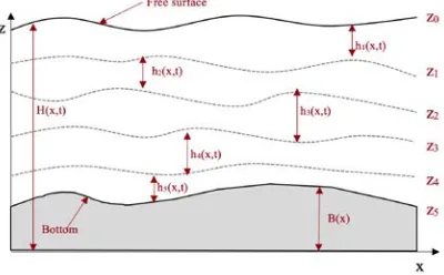
Equations of single-layer shallow water with variable density, with regard to external pressure and bottom relief

In the case of one spatial measurement, we write out the integral conservation (balances) laws for an arbitrary subdomain x∈

[

x x₁, ₂

]

(Fig. 1). We introduce the following notation:

2 2 2

1 1 1

, ρ , ρ , ,

x x x

x x x

V =

∫

hdx M =

∫

hdx Π =

∫

uhdx h=H−B

where V is an area occupied by liquid; M is a mass; П is momentum H(x, t) is a free surface; B(x) is a bottom relief; h(x, t) is a layer thickness; ρ(x, t) is a density;

u(x, t) is horizontal velocity of liquid.

The equation for variation of the area occupied by the liquid has the following form

2 2

2 1

1 1

.

x x

x x

x x

V hu

hdx uh uh dx

t t x

∂ ₌ ∂ _{= − + = −} ∂

∂ ∂

∫

∫

∂

Fig. 1. One-layer model

The variation of mass and momentum is described respectively by the equations

(

) (

)

2 2

2 1

1 1

2

2 1

1

2 2

1 1

2 2 2 2

ρ

ρ ρ ρ ,

ρ ρ ρ / 2 ρ ρ / 2

.

x x

x x

x x

x

T _x T _x

x

x x

B T

x x

M hu

hdx uh uh dx

t t x

uhdx u h gh P h u h gh P h t t

B H

P dx P dx

x x

∂ ∂ ∂

= = − + = −

∂ ∂ ∂

∂Π ₌ ∂ _{= − + + + + + −}

∂ ∂

∂ ∂

− +

∂ ∂

∫

∫

∫

∫

∫

Hereg is a free fall acceleration; PT is a pressure on a free surface; PB = PT + ρgh

is a pressure on the bottom.

The corresponding conservation laws in differential form follow from the given integral equations:

2 2

ρ ρ

0, 0,

ρ ρ ρ

. 2

T

T B

h hu h hu

t x t x

P h

uh hu g h H B

F P P

t x x x x x

∂ ₊∂ ₌ ∂ ₊∂ ₌

∂ ∂ ∂ ∂

∂

∂ ₊∂ ₊ ∂ _{+ = =} ∂ ₋ ∂

∂ ∂ ∂ ∂ ∂ ∂

After some transformations these equations can be represented as

(

)

(

)

φ φ

,φ ,ρ, T, 0,0, ρ ,

d h u d F h

t x

∂ ∂

+ × = = =

∂ A ∂

  _{  }

where

( )

1

0

0 0 , .

ρ ρ

2ρ

T

T B

B

u h

P

H B

u F P P h

x x x

gh

P h u

x

−

 

 

  _{∂ ∂ ∂}

=  = − −

∂ ∂ ∂

 _∂ 

 

 _∂ 

 

A

All matrix A eigenvalues are valid:

1 2 3

λ = +u c, λ = −u c, λ =u, c= PB ρ,

(

)

(

)

(

)

(

)

ρ ρ _{ρ ,}

2ρ 2ρ

ρ ρ _{ρ ,}

2ρ 2ρ

ρ ρ

0.

u c h gh u c h gh

u c F h

t h t c t x h x c x u c h gh u c h gh

u c F h

t h t c t x h x c x u

t x

∂ ₊ ∂ ₊ ∂ _{+ +} ∂ ₊ ∂ ₊ ∂ ₌

 _{∂ ∂ ∂}  _{∂ ∂ ∂} 

   

∂ ₋ ∂ ₋ ∂ _{+ −} ∂ ₋ ∂ ₋ ∂ ₌

 _{∂ ∂ ∂}  _{∂ ∂ ∂} 

   

∂ ∂

+ =

∂ ∂

Equations of multilayer shallow water with variable density with regard to external pressure and bottom relief

The equations of multilayer shallow water with variable density in the absence of mass and momentum exchange between the layers can be represented as the sum of single-layer equations connected by pressure and reaction forces affecting the interface (Fig. 2):

( )

(

)

(

)

(

2

)

( )

2

(

)

1 1

1 1 1 1

ρ ρ

0, 0,

ρ ρ

ρ

0, 2

1,..., , , , , ρ .

k k k k k

k k

k k k k k

k k

N k k k k k k k

hu hu

h h

t x t x

hu h

hu g h P Z Z

P P

t x x x x x

k N Z H Z B h Z Z P P g h

+ +

+ + +

∂ ∂

∂ _{+ =} ∂ _{+ =}

∂ ∂ ∂ ∂

∂ ∂

∂ ∂ ∂ ∂

+ + + + − =

∂ ∂ ∂ ∂ ∂ ∂

= = = = − = +

(1)

Here k is alayer number counted from the free surface; Zk is the coordinates of

the upper boundary of the layer; P1 = PT is an external pressure on a free surfaceZ₁.

The so-called simple form of the system of equations (1) will have the form:

(

1 1 1

)

ψ ψ

, ψ , , , ρ , , ρ , , ,_{N N N} T,

D h h u u

t x

∂ _{+ ×}∂ _{= =}

∂ G ∂

  _{ }

  

where G is a matrix of N × N dimensions and D is some right part. It is known well that already at N = 2 the matrix Gcan have complex roots and the system will not be unconditionally hyperbolic [9], which gives rise to known computational difficulties. For a larger number of layers the situation is exacerbated. Already in the presence of two layers the calculation of the eigenvalues of the matrix (4 × 4) is a rather difficult task. With a large number of layers it becomes practically insoluble and the direct use of balance-characteristic methods [23] is impossible. For overcoming this difficulty we use a technique that we will call the hyperbolic decomposition of the problem.

Fig. 2. Multilayer model

If we consider the forces affecting the interface to be external, then (1) can be represented as:

(

)

(

)

φ φ

,φ ,ρ , T, 0,0, ρ , 1,..., ,

k k

k dk k hk k uk dk Fk khk k N

t x

∂ ∂

+ × = = = =

∂ A ∂

  _{  }

where

( )

1 1 1

1

0

0 0 , ,

ρ

2ρ

k k

k k k

k k k k k k

k

k k k

k

u h

Z Z P

u F P P h

x x x

gh

P h u

+ + −

+

 

 

  _{∂ ∂ ∂}

 

= = − −

∂ ∂ ∂

 

 

 

 

A

which leads to a system of independent characteristic equations:

(

)

(

)

(

)

(

)

ρ ρ _{ρ ,}

2ρ 2ρ

ρ ρ _{ρ ,}

2ρ 2ρ

ρ ρ

0.

k k k k k k k k k

k k k k k

k k k k k k

k k k k k k k k k

k k k k k

k k k k k k

k k

k

u c h gh u c h gh

u c F h

t h t c t x h x c x

u c h gh u c h gh

u c F h

t h t c t x h x c x

u

t x

∂ ₊ ∂ ₊ ∂ _{+ +} ∂ ₊ ∂ ₊ ∂ ₌

 _{∂ ∂ ∂}   _{∂ ∂ ∂} 

   

∂ ₋ ∂ ₋ ∂ _{+ −} ∂ ₋ ∂ ₋ ∂ ₌

 _{∂ ∂ ∂}   _{∂ ∂ ∂} 

   

∂ ₊ ∂ ₌

∂ ∂

(2)

This makes it possible to use algorithms that have proven themselves in the single-layer case for the numerical solution of a complete system of multilayer equations. The incorrectness of the complete system will not disappear and will manifest itself in high-frequency distortion of the boundaries. Using special filters the distortion can be significantly reduced while maintaining the approximation order and without violating the conservation laws.

CABARET scheme for the layered solution of the equations of multilayer shallow water

We cover the domain of the problem solution with an uneven computational grid with xi, i = 1, Nx coordinates of the nodes. In the nodes at the initial moment of

time we set the vertical coordinates of η_{k i,} layers:

( )

0

( )

0 0

( )

0

, 1 1

η , , , 1,..., .

k _i k i _i i N _i i x

Z = Z =H Z ₊ =B i= N

The constant coordinates of the nodes along the x axis and the time-dependent vertical coordinates of n_,

k i

Z layers determine the computational grid on the (x, z) plane.

Two types of variables are used in the CABARET scheme: flux and conservative [22] ones. Flux variables refer to the midpoints of the vertical faces of computational cells, conservative ones – to their centers. Flux variables related to the layer with the number k will be denoted as ρ ,n_, n_, , n_, n_, n_1,

conservative – as ρn_{, 1/ 2}, n_{, 1/ 2}, n_{, 1/ 2}

k i+ uk i+ hk i+ . At the initial moment flux variables are set. Conservative variables are determined by flux ones as follows:

(

)

(

)

(

)

0 0 0 0 0 0

, 1/ 2 , , 1 , 1/ 2 , , 1

0 0 0

, 1/ 2 , , 1

ρ 0,5 ρ ρ , 0,5 ,

0,5 .

k i k i k i k i k i k i

k i k i k i

u u u

h h h

+ + + +

+ +

= + = +

= +

The computational algorithm consists of the following elements: calculation of conservative variables on an intermediate time layer according to conservative finite-volume schemes (phase 1); calculation of flux variables on a new time layer by extrapolation of local Riemann invariants (phase 2); calculation of conservative variables on a new layer using finite-volume schemes (phase 3).

Phase 1. In order to calculate the intermediate conservative variables, we use:

( )

( )

( )

( )

(

)

(

)

(

)

(

)

(

) (

)

(

) (

)

1/ 2 , , , , 1/ 2 , , , ,

1/ 2 2 2

1/ 2 1/ 2

, , , ,

, 1 , 1 , 1 , 1 , , , ,

0, τ 2 ρ ρ ρ ρ 0, τ 2 ρ ρ ρ ρ τ 2 2 2 n n n n

C k C k R k L k

n n n n

C k C k R k L k

n n

n n n n

k k k k

C k C k R k L k R L

n n n n n n n n

R k L k R k L k R k L k R k L k

hu hu h h

x

h h hu hu

x

hu hu

hu hu h P h P

x x

P P Z Z P P Z Z

x + + + + + + + + + − − + = ∆ − − + = ∆ − − − + + + ∆ ∆ + − + − + −

∆ ∆x =0,

whereP_{k+1/ 2}=

(

P+0,5ρgh

)

_k. These equations have the first order of approximation in time and the second in spatial variable.

Phase 2. In order to find new flux variables, a linearized system of characteristic equations (2), which can be written in the following form, is used:

(

)

(

)

1/ 2 1/ 2

1/ 2 1/ 2

1/ 2 1/ 2

1/ 2 1/ 2

1/ 2 1/ 2

1/ 2 1/ 2

1 ρ 2ρ ρ _{ρ ,} 2ρ n n

k k k k k

k i k k i

n n

n _{k k k k k} n

k k _i k k k _i

k _i k k _i

k k

k i

u c h gh

t h t c t

u c h gh

u c F h

x h x c x

u c t h + + + + + + + + + + + + + _{∂   ∂   ∂}   +_{ } +_{ } +  ∂ _{ } ∂ _{ } ∂    _{∂   ∂   ∂}    + _ + _ +_{ } +_{ } = _ _  ∂ _{ } ∂ _{ } ∂      ∂ −   ∂ _{ }

(

)

(

)

[ ]

1/ 2 1/ 2

/ 2 1/ 2

1/ 2 1/ 2

1/ 2 1/ 2

1/ 2 1/ 2

1/ 2 1/ 2

1/ 2 1/ 2 ρ 2ρ ρ _{ρ ,} 2ρ ρ ρ 0, n n

k k k

k k i

n n

n _{k k k k k} n

k k _i k k k _i

k i k k i

n

k k

k i

h gh

t c t

u c h gh

u c F h

x h x c x

u t x + + + + + + + + + + + + +  _{∂   ∂}   −_{ } +  ∂ _{ } ∂    _{∂   ∂   ∂}    + _ − _ −_{ } −_{ } = _ _  ∂ _{ } ∂ _{ } ∂    ∂ ∂ + = ∂ ∂

which can be written down as

( )

( )

( )

( )

( )

( )

( )

( )

( )

( )

( )

( )

1/ 2 1 , 1/ 2 1/ 2 1 , 1/ 2

1 1/ 2 1, 1/ 2 1/ 2 2 , 1/ 2 1/ 2 2 , 1/ 2

2 1/ 2 2, 1/ 2

1/ 2 3 , 1/ 2 1/ 2 3 1/ 2

3 1/ 2 3, 1/ 2

λ ,

λ ,

λ ,

n n

k i k i

k

i i

n n

k i k i

k

i i

n n

k i k

k i i I I Q t x I I Q t x I I Q t x + + + + + + + + + + + + + + + + + + ∂ ∂ + = ∂ ∂ ∂ ∂ + = ∂ ∂ ∂ ∂ + = ∂ ∂ (3) where

( )

(

)

( )

(

)

( )

( )

( )

( )

(

)

( )

1/ 2 1/ 2 1/ 2 1/ 2 1/ 2 1/ 2

1 1/ 2 1/ 2 2 1/ 2 1/ 2 3 1/ 2 1/ 2

1/ 2 1/ 2 1/ 2 1/ 2

1, _{1/ 2} 2, _{1/ 2 1/ 2} 3, _{1/ 2}

λ , λ , λ ,

ρ , 0,

n n n n n n

k k k k k

i i i i i i

n n n n

k _i k _i k k k _i k _i

u c u c u

Q Q F h Q

+ + + + + + + + + + + + + + + + + + + + = + = − = = = _ _ =

( )

I1 k i,+1/ 2,

( )

I2 k i,+1/ 2,

( )

I3 k i,+1/ 2 are local Riemann invariants in a cell i + 1/2 of k

layer at time interval

[

t t_n, _n+1

]

:

( )

( )

( )

1/ 2 1/ 2

1 , 1/ 2 1/ 2, 1/ 2, 2 , 1/ 2 1/ 2 1/ 2

1/ 2, 1/ 2, 3 , 1/ 2

1/ 2 1/ 2

1/ 2 1/ 2

1/ 2, 1/ 2,

1/ 2 1/ 2

ρ ,

ρ , ρ ,

, .

2ρ

n n

k i k k i k k

k i k i

n n

k i k k i k k k i k

n n

n k n k

i k i k

k i k k i

I u G h D I

u G h D I

c gh G D h c + + + + + + + + + + ₊ + + + + + + + + = + + = = − − =     =_{ } =_{ }    

Note that at variable density the eigenvalues of

A

_kmatrix remain the same as with constant density [24], while left eigenvetctors are modified which leads to the appearance of an additional term proportional to the density in local invariants.

The first action of phase 2 consists in calculating the preliminary values of local invariants on a new time layer using the linear extrapolation method taking

into account the sign of the characteristic velocity

( )

λ_m n_i++_{1/ 2}1/ 2,m=1, 2, 3:

( )

( )

( )

( )

( )

( )

( )

( )

( )

( )

( )

( )

( )

1/ 2 1/ 2 1/ 2

, 1/ 2 , , 1/ 2 , 3/ 2

1 _{1/ 2 1/ 2 1/ 2}

, 3/ 2 , 2 , 3/ 2 , 1/ 2

, 1

1/ 2 1/ 2 1/ 2 1/ 2

, 3/ 2 , 1/ 2 , 3/ 2 , 1/ 2

2 λ 0 λ 0,

2 λ 0 λ 0,

/ 2 λ λ

n n n n

m k i m k i m k i m k i

n _{n n n n}

m _{k i} m k i m k i m k i m k i

n n n n

m k i m k i m k i m k i

I I if and

I I I if and

I I if

+ + + + + + + _{+ + +} + + + + + + + + + + + + +

− > ≥

= − < ≤

 ₊  _×    0.       < 

( )

{

( ) ( ) ( )

}

( )

{

( ) ( ) ( )

}

( )

{

( )

( )

}

( )

{

( )

( )

}

, _{1/ 2} , ₁ , _{1/ 2} , , _{1/ 2} , ₁ , _{1/ 2} ,

, ₁ , _{1/ 2} , _{3/ 2}

, ₁ , _{1/ 2} , _{3/ 2}

min min , , ,

max max , , ,

min min min , min ,

max max max , max

n n n

m k _i m k _i m k _i m k _i

n n n

m k _i m k _i m k _i m k _i

m k _i m k _i m k _i

m k _i m k _i m k _i

I I I I

I I I I

I I I

I I I

+ + + + + + + + + + + + = = = =

and the right sides of the transport equations (3) from the known left sides:

( )

(

)

( )

( )

( )

( )

( )

( )

1/ 2

1/ 2 , 1/ 2 , 1/ 2 1/ 2 , 1 , 2

, 1/ 2 1 1/ 2

1/ 2 3, _{1/ 2}

λ τ ,

τ 2

= 1, 2, = 0.

n n n n

m m m m

n k i k i n k i k i

m k i i

n k _i

I I I I

Q O x m Q + + + + + + + + + + − − = + + ∆

From the transport equations by characteristics (3) it follows that if

( )

1/ 2

, _{1/ 2}

n

m k _i

Q ₊+ values are equal to zero and the Courant – Friedrichs – Lewy number

(CFL) is less than unity, then the following conditions must be satisfied:

( )

( )

( )

( )

( )

( )

( )

( )

( )

( )

( )

( )

( )

1/ 2 1/ 2

, 1/ 2 , 1/ 2 , 1/ 2 , 3/ 2

1 1/ 2 1/ 2

, ,

, 1 3/ 2 3/ 2 , 3/ 2 , 1/ 2

1/ 2 1/

, 1 , 1 , 3/ 2 , 1/ 2

min , max λ 0 λ 0,

min , max λ 0 λ 0,

min , max λ λ

n n

m k i m k i m k i m k i

n n n

m k i m k i m k i m k i m k i

n n

m k i m k i m k i m k i

I I if and

I I I if and

I I if

+ + + + + + + + + + + + + + + + + + + +

  _{> ≥}

 

 

∈ _{ } < ≤

  ×

  2 0.

      < 

For non-zero

( )

_, 1/ 2

1/ 2

n

m k _i

Q ₊+ intervals of permissible values are shifted:

( )

( )

( )

( )

( )

( )

1/ 2 , _{1/ 2} , _{1/ 2} , _{1/ 2} 1/ 2 , _{1/ 2} , _{1/ 2} , _{1/ 2}

max max τ ,

min min τ .

n

m k _i m k _i m k _i

n

m k _i m k _i m k _i

I I Q

I I Q

+ + + + + + + + = + = +

Correction of

( )

1

, 1

n m _{k i}

I +

+

 invariants consists in the following: if the preliminary value

of

( )

1

, 1

n m _{k i}

I +

+

 invariant satisfies these inequalities, then the invariant does not change;

if not, it is assigned a value corresponding to the closest boundary of the allowable interval. According to the adjusted values of local invariants on a new time layer from the system of equations

( )

( )

( )

( )

( )

( )

( )

( )

( )

( )

1 1

3

1 , 1

1 * 1 * 1 1

1, 1, 1

1 1 1 , 1

1 _* 1 _* 1 1

2, 2, 2

1 1 1 , 1

ρ ,

ρ ,

ρ

n n

k i k i

n n n n

k i k k i k k i k i

n n n n

k _i k k _i k k _{i k i}

I

u G h D I

u G h D I

+ + + + + + + + + + + + + + + + + + + + = + + = − − =

new flux variables are calculated:

( )

( )

( )

( )

( )

( )

( )

( )

1 1

* * * *

1, 2 2, 1

1 1 1 , 1 , 1

3 * *

1 , 1 1

1, 2,

1 1

* *

1 2

1 , 1 , 1

* * 1 1, 2, ρ , , , n n k k

n n n k i k i

k i k i k i

k k

n n

n k i k i

k i

k k

G I G I

I u G G I I h G G + + + + + + + + + + + + + + + + + = = + − = + where

( )

_* 1

( )

1 _*

( )

1

( )

_* 1

( )

1 _*

( )

1 1 , 1 1 , 1 1, ρ 1, 2 , 1 2 , 1 2, ρ 1

n n n n n n

k k k k

k i i k i i

k i k i

I + I +₊ D ₊+ I + I +₊ D ₊+

+ = − + = + ,

* * 1,k, 2,k

G G take the values:

(

)

(

)

( )

( )

(

)

( )

( )

(

)

( )

( )

1/ 2 1/ 2

1/ 2 1/ 2

1/ 2, 1/ 2, , 1/ 2 , 3/ 2

1/ 2 1/ 2

* * 1/ 2 1/ 2

, , 3/ 2, 3/ 2, , 1/ 2 , 3/ 2

1/ 2 1/ 2 1/ 2

1, 1, , 1/ 2 , 3/ 2

, λ 0 λ 0,

, , λ 0 λ 0,

, λ λ

n n

n n

i k i k m k i m k i

n n

n n

m k m k i k i k m k i m k i

n n

n n

i k i k m k i m k i

G D if and

G D G D if and

G D if

+ + + + + + _{+ +} + + + + + + + + + + + + + + _{+ +} > ≥

= < ≤

×

(

)

(

)

1/ 2

1/ 2 1/ 2 1/ 2 1/ 2 1/ 2 1/ 2 1, 1/ 2, 3/ 2, 1, 1/ 2, 3/ 2,

0,

1, 2, n n n / 2, n n n / 2.

i k i k i k i k i k i k

where m G₊+ G₊+ G₊+ D₊+ D₊+ D₊+

     ≤  = = + = +

Filtering of flux variables. In the areas of hyperbolicity loss, short-wave disturbances are generated. To regularize the solution, the calculated flux variables are filtered:

( )

( )

(

)( ) ( )

( )

( )

( )

( )

(

)

( ) ( )

( )

( )

( )

( )

( ) ( )

(

)

(

)

( )

(

)

( )

( )

( )

1 1 1 1 1 1

1 1

1 1 1 1 1 1

1 1

1 1 1 1 1 1

1

1 1

σ 1 σ , / 2,

ρ σ ρ 1 σ ρ , ρ ρ ρ / 2,

, σ 1 σ ,

,

n n n n n n

k i u k i u k i k i k i k i

n n n n n n

k _i k _i k _i k _i k _i k _i

n n n n n n

k _i k i k _i k _i h k i h k _i

n

n n n

k i k i k i k i

u u u u u u

h h h h h h

h h h h

ρ ρ + + + + + + + − + + + + + + + − + + + + + + + + +   = + − =_ + _   = + − =_ + _ = + ∆ ∆ = ∆ + − ∆ ∆ = − ∆     

(

)

1

(

)

1

[ ]

1 1 / 2, σ , σ , σ 0,1 .

n n

k i k i u h

h h ρ

+ +

+ −

 

= ∆_ + ∆ _ ∈

(4)

Regularized thicknesses of the layers determine new values of their levels:

(

₁

) (

₁

)

( )

1

(

₁

)

₁

(

₁

)

1 , 1 , 1 , 1,..., , 1,..., .

n

n n n n n

k _i k _i k _i N _i i i _i x

Z + = Z ₊+ + h + Z +₊ =B H + = Z + k = N i= N

It should be noted that nonlinear correction of local invariants does not always occur, but only in the areas of sharp gradients. Filters (4) do not lead to a decrease in the approximation order.

( )

( )

( )

( )

(

)

(

)

(

)

(

)

(

) (

)

(

)

(

)

1 1

1 1/ 2

, , , ,

1 1/ 2 1 1

, , , ,

1 1

1 1/ 2 2 2 * *

1/ 2 1/ 2

, , , ,

1 1 1

, 1 , 1 , 1 , 1

0, τ 2

ρ ρ ρ ρ

0, τ 2

ρ ρ

ρ ρ

τ 2

2

n n

n n

C k C k R k L k

n n n n

C k C k R k L k

n n

n n

k k k k

C k C k R k L k R L

n n n n

R k L k R k L k

hu hu h h

x

h h hu hu

x

hu hu

hu hu h P h P

x x

P P Z Z

σ σ

+ +

+ +

+ + + +

+ +

+ +

+ +

+ + +

+ + + +

− −

+ =

∆

− −

+ =

∆ −

− −

+ + +

∆ ∆

+ −

+

1 1 1 1 1

, , , ,

0, 2

n n n n

R k L k R k L k

P P Z Z

x x

+ + ₊ + + ₋ +

− =

∆ ∆

where fσ*=2σfn+1+ −(1 2σ) , σ 1/ 2, 3 .fn ∈

[

]

Phase 3 difference equations approximate the initial differential equations with the second order in the spatial variable and with the first in time. If we add these equations to the ones of phase 1, then the resulting system at σ = 0.5 will have

a second order of approximation and, in the absence of filtering (σ_u =σ_h=σ_ρ =0), have the property of temporary reversibility. By changing the parameter σ, one can control the dissipative properties of the scheme. At σ 1> the scheme becomes super implicit [23], although the computational algorithm remains explicit. This algorithm at constant density is balanced: the resting state above an arbitrary bottom relief is not violated [24].

The selection of time step value. The stability condition for CABARET scheme for each layer has the form [22]

( )

_{1/ 2}

( )

_{1/ 2}

1/ 2

τ 1, n

n

k i k i

i

c u

x

+ +

+

 ₊ 

 _{ ≤}

∆

whence

( )

1/ 2

( )

1/ 2 ,

1/ 2 1/ 2

1

τ min _n .

n i k

k i k i

CFL

c ₊+ u ₊+

= ×

 ₊ 

 

Rearrangement of layer boundaries. Filtering of flux variables without affecting conservative values does not make the complete task correct for sufficiently long periods of time. We have to correct conservative variables, which leads to the mass and momentum exchange between the layers.

The grid reconstruction in the proposed algorithm is carried out twice in one time cycle. The first time is after calculating the conservative variables on the intermediate layer in phase 1, the second time – after phase 3.

In phase 1 intermediate conservative velocities u_in++_{1/ 2,}1/ 2_kand layer thicknesses 1/ 2

1/ 2,

n i k

h₊+ are calculated. Along them new heights of the interfaces

1/ 2 1/ 2 1/ 2 1/ 2 1/ 2

1/ 2, 1/ 2, 1 1/ 2, , 1/ 2, 1 1/ 2, 1 1/ 2, 1/ 2,1= 1/ 2 , 1,..., .

n n n n n n n

i k i k i k i N i N i i i

Z₊+ =Z_{+ +} +h₊+ Z₊+ ₊ =Z_{+ +} =B₊ Z₊+ H₊+ k = N

are found. In general case these coordinates are not final and are subject to correction.

We consider three ways to set Zˆ_in₊+_{1/ 2,}1/ 2_k that does not exhaust all the possibilities.

1. The heights are not rearranged and 1/ 2 1/ 2 1/ 2, 1/ 2,

ˆn n

i k i k

Z₊+ =Z₊+ . In this case, there is no mass and momentum exchange between the layers and the problem remains incorrect.

2. New heights of the interfaces are set so that the ratio of the layer thicknesses in each vertical column remains the same (sigma-coordinate):

(

)

1/ 2 1/ 2 1/ 2 1/ 2 1/ 2, 1/ 2, 1 1/ 2 1/ 2 1/ 2 1/ 2

1

ˆ ˆ

ˆ ˆ _{σ , ,}

1,..., , σ 0, σ .

n n n n n

i k i k k i i N i i

N

k k

k

Z Z h h H B N

k N N

+ + + +

+ + + + + + +

=

= + = −

= >

∑

=

3. The lower boundary of k =s, N ≥ >s 1layer remains motionless (Euler), all the boundaries of the layers at k>s are also motionless and the thicknesses of the layers at k<s have the specified proportions (sigma-coordinate):

(

)

1/ 2 0 1/ 2 1/ 2 1/ 2

1/ 2, 1 1/ 2, 1 1/ 2, 1/ 2, 1 1/ 2, 1/ 2 1/ 2 0

1/ 2, 1/ 2 1/ 2, 1

1

ˆ _{, ,} ˆ ˆ _{σ , 1,..., ,}

, 1,..., , σ 0, σ .

n n n n

i k i k i k i k k i k

s

n n

i k i i k k k

k

Z Z k s Z Z h k s

h H Z s k s s

+ + + +

+ + + + + + + +

+ +

+ + + +

=

= ≥ = + =

= − = >

∑

=





The conservation laws lead to the mass and momentum exchange between the layers in the second and third cases. The fluxes between the layers can be approximated with both the first and second order of accuracy.

The first order accuracy fluxs are calculated by the donor cell method, which is as follows. We consider the lowest layer (k=N ). If hˆ_in₊+_{1/ 2,}1/ 2_N ≤h_in₊+_{1/ 2,}1/ 2_N, then the lower layer thickness decreases by the value 1/ 2 1/ 2 1/ 2

1/ 2, 1/ 2, ˆ 1/ 2, 0

n n n

i N i N i N

h₊+ h₊+ h₊+

∆ = − ≥ and

a part of its mass 1/ 2 1/ 2

1/ 2 ρ 1/ 2, 1/ 2, 1/ 2

n n

i i N i N i

m_{+ +}+ h₊+ x₊

∆ = ∆ ∆ and momentum

( )

1/ 2 1/ 2 1/ 2 1/ 2, 1/ 2, 1/ 2, 1/ 2 1/ 2 ρ

n n n

i N i N i N i i

mu _{+ +}+ u₊+ h₊+ x₊

∆ = ∆ ∆ enters the cell of the layer lying above. As a result, we obtain:

1/ 2 1/ 2 1/ 2 1/ 2 1/ 2 1/ 2 1/ 2, 1/ 2, 1/ 2, 1/ 2, 1/ 2, 1/ 2 1/ 2,

1/ 2 1/ 2 1/ 2 1/ 2 1/ 2, 1 1/ 2, 1 1/ 2, 1/ 2, 1/ 2

1/ 2, 1 1/ 2

1/ 2, 1 1/ 2,

ˆ ˆ

ˆ ˆ

ρ ρ , , ,

ρ ρ

ˆ ρ

n n n n n n

i N i N i N i N i N i i N

n n n n

i N i N i N i N

n

i N n n

i N i N

u u Z B h

h h

h h

+ + + + + +

+ + + + + + +

+ + + +

+ − + − + +

+

+ − +

+ − +

= = = +

+ ∆

=

+ ∆ 1/ 2

1/ 2 1/ 2 1/ 2 1/ 2 1/ 2 1/ 2 1/ 2, 1 1/ 2, 1 1/ 2, 1 1/ 2, 1/ 2, 1/ 2, 1/ 2

1/ 2, 1 1/ 2 1/ 2 1/ 2 1/ 2 1/ 2, 1 1/ 2, 1 1/ 2, 1/ 2,

,

ρ ρ

ˆ .

ρ ρ

n n n n n n

i N i N i N i N i N i N

n

i N n n n n

i N i N i N i N

u h u h

u

h h

+

+ + + + + +

+ − + − + − + + +

+

+ − + + + +

+ − + − + +

+ ∆

=

+ ∆

In the opposite case when 1/ 2 1/ 2 1/ 2, 1/ 2,

ˆn n

i N i N

h++ ≥h++ , the upper cell gives up part of its mass

1/ 2 1/ 2 1/ 2 1/ 2 1/ 2 1/ 2 1/ 2, 1 1/ 2, 1 1/ 2, 1 1/ 2, 1 1/ 2, 1/ 2 1/ 2,

1/ 2 1/ 2 1/ 2 1/ 2 1/ 2, 1/ 2, 1/ 2, 1 1/ 2, 1/ 2

1/ 2, 1/ 2

1/ 2, 1/ 2,

ˆ

ˆ ˆ

ρ ρ , , ,

ρ ρ

ˆ ρ

n n n n n n

i N i N i N i N i N i i N

n n n n

i N i N i N i N n

i N n n

i N i N

u u Z B h

h h

h h

+ + + + + +

+ − + − + − + − + + +

+ + + +

+ + + − +

+

+ + +

+ +

= = = +

− ∆

=

− ∆ 1/ 2

1/ 2 1/ 2 1/ 2 1/ 2 1/ 2 1/ 2 1/ 2, 1/ 2, 1/ 2, 1/ 2, 1 1/ 2, 1 1/ 2, 1/ 2

1/ 2, 1/ 2 1/ 2 1/ 2 1/ 2 1/ 2, 1/ 2, 1/ 2, 1 1/ 2,

,

ρ ρ

ˆ .

ρ ρ

n n n n n n

i N i N i N i N i N i N n

i N n n n n

i N i N i N i N

u h u h

u

h h

+ + + + + +

+ + + + − + − +

+

+ + + + +

+ + + − +

− ∆

=

− ∆

It should be pointed out that in the method of donor cells the densities and velocities are considered piecewise constant functions along the vertical.

The second-order accuracy fluxes are found from the condition according to which the density and horizontal velocity are linear functions on the segment connecting the midpoints of neighboring layers. We consider the cells of two adjacent layers (with the indices B is the lower layer, T is the upper layer). By

, required

B B

z h h

∆ = − we denote the variation of the boundary between the layers, by ∆x– the width of these cells, by ∆ ∆m p, – the mass and momentum variation of the layers. Then we get the following expressions:

(

₎₍

₎

(

₎₍

₎

ρ ρ

1

ρ ,

2 / 2

ρ ρ

1

ρ .

2 / 2

T B

B B

T B

T T B B

B B B

T B

m z x h z z x

h h u u

p u z x h z z x

h h

−

∆ = ∆ ∆ + + ∆ ∆ ∆

+ −

∆ = ∆ ∆ + + ∆ ∆ ∆

+

New values of densities and velocities of layers are calculated by the following formulas:

,required ,required , required , required

ρ ρ

ˆ ˆ

ρ , ρ ,

ρ ρ

ˆ , ˆ .

ˆ ˆ

ρ ρ

T T B B

T B

T B

T T T B B B

T B

T T B B

h x m h x m

h x h x

h u x p h u x p

u u

h x h x

∆ + ∆ ∆ − ∆

= =

∆ ∆

∆ + ∆ ∆ − ∆

= =

∆ ∆

Recalculation of conservative variables on other layers is carried out similarly, from the lower layers to the upper ones. Then, the corrected conservative variables and layer thicknesses marked with fˆn+1/ 2symbol are taken as final values _fn+1/2_and

are used in the next phase 2. A similar correction of conservative variables is also carried out after phase 3.

Artificial (turbulent) viscosity. In gas dynamics problems the artificial viscosity method is used to regularize the numerical solution in the presence of shock waves [25]. A difference operator is added to the numerical algorithm, which approximates the so-called second – bulk viscosity, the coefficient at which is proportional to the spatial step of the grid and is found from the condition of the fastest attenuation of the highest frequency harmonic [26]. In the areas of rarefaction waves where the velocity divergence is positive, the artificial viscosity is zeroed. This provides the monotonicity of the numerical solution on compression waves and does not spoil rarefaction waves.

In the case of multilayer hydrodynamics, the inclusion of linear artificial viscosity is reduced to the modification in phase 1 and phase 3 of the flux grid pressure function on the vertical faces of the computational grid. For phase 1:

(

)

(

*

)

(

)

*

( )

(

)

1/ 2 1/ 2 1/ 2 , , , 1/ 2 , 1/ 2 , 1/ 2 , 1/ 2

* ,

, 1/ 2 , 1/ 2

θ ρ ,

θ 0,

θ

0 0,

n

n n n n n

k j k j k j k j k j k j k j

n n

k j k j

k j n n

k j k j

P P P с u u

if u u if u u

+ + + + −

+ −

+ −

⇐ = − −

 − <



=  _{− ≥}



where с_j = P_k+1 ρ_k is a local speed of sound, θ 1 is a dimensionless parameter.

For phase 3:

(

)

1

(

*

)

1

(

)

1 *

( )

1/ 2

(

1/ 2 1/ 2

)

1/ 2 1/ 2 1/ 2 , , , 1/ 2 , 1/ 2

1/ 2 1/ 2 , 1/ 2 , 1/ 2 *

, 1/ 2 1/ 2

, 1/ 2 , 1/ 2

θ ρ ,

θ 0,

θ

0 0.

n

n n n n n

k j k j k j k j k j k j k j

n n

k j k j

k j n n

k j k j

P P P с u u

if u u if u u

+

+ + + + +

+ + + + −

+ +

+ −

+ +

+ −

⇐ = − −

 − <



=  _{− ≥}



A generalization for the case of two spatial dimensions. A transition from the one-dimensional algorithm described above to the two-dimensional multilayer one is carried out similarly to that described in [27] for single-layer shallow water on a sphere. The consideration of Coriolis force in the CABARET scheme, which operates with two types of variables (conservative and flux), does not cause difficulties and does not impose additional restrictions on the time step.

Algorithm Verification

The purpose of verification is to check the algorithm for the absence of programming errors, computational stability and convergence on problems that can be compared with an analytical solution or with a numerical solution obtained by other authors. The proposed algorithm coincides with that described in [24] for one layer and constant density. In the presence of one layer and variable density the new multilayer algorithm coincides with that described in [28].

The features of multilayer models are already evident in problems with two or three layers [29–31]. In these works, the examples of calculations of model problems, on which our methodology was tested, are given. It should be noted that in the mentioned papers the results of the solution for a certain moment of time on fixed computational grids are presented, and the behavior of the numerical solution on large time intervals and on the grids of various densities is not studied.

We will illustrate the stability problems of the numerical solution of multilayer shallow water equations in the absence of mass and momentum exchange between layers on the two-layer problem of A. Kurganov from [30]. The initial data (Fig. 3) are as follows:

( )

( )

₍

₎

( )

( )

₍

₎

1 1 1

2 2 2

1 2 1,

,0 0, 4,ρ 0,98, ,0

1 0, 25sin 2 1,

1 2 1,

,0 0, 4,ρ 1, ,0

1 0, 25sin 2 1.

if x

u x h x

x if x if x

u x h x

x if x π

π

 ≥ ≥



= = _{= }

− <



 ≥ ≥



= − = _{= }

+ <

Bottom reliefB x( )= −2,x∈ −

[

2, 2 ,

]

g=10. Computational grid – 801 node on x -axis.

Fig. 3. Initial conditions

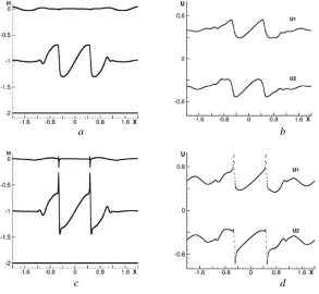
The results of calculations according to the CABARET scheme are shown in Fig. 4. The calculations were carried out with the following parameters:

*

ρ

σu =σh =σ =2 3, σ =3, θ 0, = CFL=0,3. Graphs of the layer interfaces and their velocities at time t = 0.5 are given in Fig. 4, a, b. They practically coincide with those presented in [30]. When the calculation is continued, the thickness of the layers degenerates and at t = 0.65 the calculation ceases (Fig. 4, c, d).

a b

c d

Fig. 4. Calculation on the 800 cell grid by the CABARET scheme: boundaries and velocity of the layers at t = 0.5 (a, b) and t = 0.65 (c, d)

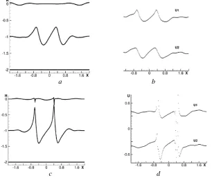
If we use a denser grid with the number of nodes 1601, then the loss of stability occurs much earlier. On a coarser grid (at N = 201) the instability develops more slowly (Fig. 5) but poor problem conditioning inevitably leads to an abortion of calculation.

The computational grid rearrangement and the resulting exchange of mass and momentum between the layers largely regularize the problem [15, 32–34], however, in this case the proper choice of filtrering parameters and artificial viscosity remains very important.

a b

c d

Fig. 5. Calculation on the 200 cell grid by the CABARET scheme: boundaries and velocity of the layers at t = 0.5 (a, b) and t = 1 (c, d)

Calculation of the barotropic flux according to the multilayer model with regard to the mass and momentum exchange between the layers

We consider the problem of fluid oscillations in a basin with a flat bottom and a free boundary form perturbed at the initial moment. The problem parameters, initial and boundary conditions are defined as follows:

[

]

( )

(

0

)

(

)

( )

0

5, 5 , 2, , 0, 5, 5, 0, ρ 1, 10,

1 2 5 5

1 cos ,

( , ) 2 5 2 2

0 .

x B x u x t u t u t g

x

if x H x t

else π

∈ − = − = − = = = =

  ₊   _{− < <}

   

=_{   }

 

the initial moment is represented, in Fig. 6, b – the free surface at t=6and 128

x

N = number of computational cells.

a b

Fig. 6. Form of the liquid surface: a – initial conditions, b – at t = 6. Solid line denotes one-layer water, the markers – multilayer water (number of the layers N = 10)

The calculations were carried out at *

ρ

σu =σh =σ =2 / 3, σ =2, θ 0, = 0,3

CFL= parameters. As the calculation time increases and the grid thickens, the algorithm does not lose stability and demonstrates the grid convergence.

Conclusion

Multilayer hydrostatic model with a free surface excluding the mass and momentum exchange between the layers are incorrect in most cases and cannot be used in practical calculations. Rearrangement of the computational grid at each time step can regularize the problem. However, in order to provide guaranteed stability it is necessary to use filtering of flux variables and artificial viscosity simulating the turbulent mixing. Further development of the proposed model will be aimed at developing rules for the application of the described methods for regularizing the solution that minimizes the numerical dissipation.

REFERENCES

1. Marchuk, G.I., Dymnikov, V.P. and Zalesny, V.B., 1987. [Mathematical Models in

Geophysical Hydrodynamics and Methods of their Numerical Implementation]. Leningrad:

Gidrometeoizdat, 296 p. (in Russian).

2. Zalesny, V.B., Marchuk, G.I., Agoshkov, V.I., Bagno, A.V., Gusev, A.V., Diansky, N.A., Moshonkin, S.N., Tamsalu, R. and Volodin, E.M., 2010. Numerical Simulation of Large-Scale Ocean Circulation Based on the Multicomponent Splitting Method. Russian Journal of

Numerical Analysis and Mathematical Modelling, [e-journal] 25(6), pp. 581-609.

https://doi.org/10.1515/RJNAMM.2010.036

3. Marchuk, G.I., Paton, B.E., Korotaev, G.K. and Zalesny, V.B., 2013. Data-Computing Technologies: A New Stage in the Development of Operational Oceanography. Izvestiya,

Atmospheric and Oceanic Physics, [e-journal] 49(6), pp. 579-591.

doi:10.1134/S000143381306011X

4. Dotsenko, S.F., Zalesny, V.B. and Sannikova, N.K.V., 2016. Block Approach to the Simulation of Circulation and Tides in the Black Sea. Physical Oceanography, [e-journal] (1), pp. 3-19. doi:10.22449/1573-160X-2016-1-3-19

5. Zalesny, V.B., Gusev, A.V. and Fomin, V.V., 2016. Numerical Model of Nonhydrostatic Ocean Dynamics Based on Methods of Artificial Compressibility and Multicomponent Splitting. Oceanology, [e-journal] 56(6), pp. 876-887. doi:10.1134/S0001437016050167 6. Goloviznin, V.M., Zaytsev, M.A., Karabasov, S.A. and Korotkin, I.A., 2013. [New

Algorythms of Numerical Hydrodynamic for Multiprocessor Computational System].

Moscow: MSU, 467 p. (in Russian).