PHYSICAL OCEANOGRAPHY NO. 2 (2015) 69
Identification of a Pollution Source Power
in the Kazantip Bay Applying the Variation Algorithm
V.S. Kochergin, S.V. Kochergin
Marine Hydrophysical Institute, Russian Academy of Sciences, Sevastopol, Russian Federation
e-mail: [email protected]
The transport model of passive admixture in the Azov Sea is considered. On its basis the variational algorithm of identification power source pollution, including a variable in space, is implemented. The algorithm operability of optimum space distribution search of power source with measurements data is shown on a test example. Test calculations for the Kazantip Bay under east wind stress were carried out. The measurement data assimilation algorithm in the passive admixture transfer model is implemented applying gradient methods for optimal estimate retrieval. The retrieval is carried out by means of minimizing a quadratic function of prediction quality. The linked problem solving is used in the gradient of quality functional construction. On the basis of the variational method of data assimilation, the optimal estimate retrieval algorithm for pollution source power identification is constructed. In application of the algorithm, the integration of the main, linked and variational problems is implemented. The latter is solved to determine an iteration parameter when performing gradient descent. Integration problems are solved using TVD approximations. For the application of the procedure, the Sea of Azov flow fields and turbulent diffusion coefficients are obtained using the sigma coordinate ocean model (POM) under the eastern wind stress conditions being dominant at the observed period of time. Furthermore, the results can be used to perform numerical data assimilation on loads of suspended matter.
Keywords: power source identification, variation algorithm, discrepancy functional, concentration field, measurement data assimilation, the Azov Sea.
DOI: 10.22449/1573-160X-2015-2-69-76
© 2015, V.S. Kochergin, S.V. Kochergin © 2015, Physical Oceanography
Introduction. Studying the admixture distribution dynamics the application of the both contemporary mathematical models [1] and the methods of measurement data assimilation [2, 3], allowing identifying the model input parameters, is necessary. Measurement data assimilation algorithms are mainly based on the forecast quality quadratic functional minimization featuring the decline of model solution from measurement data. At the same time the passive admixture transport model acts as a limitation of the input parameter variation. In the work [4] the variation algorithm of power source identification for two-dimensional model is thoroughly considered, its efficiency in the presence of measurement data on the pollution spot periphery in case of point source effect by time constant and variable power is also shown. In the present work such approach is applied to three-dimensional model of passive admixture transport model in the Azov Sea. The task to identify the constantly acting pollution source power space variable is considered.
Variation algorithm of measurement data assimilation. Below we consider thepassive admixture transport model in σ-coordinates
σ σ
σ ∂
∂ ∂
∂ + ∂ ∂ ∂
∂ + ∂ ∂ ∂
∂ = ∂ ∂ + ∂ ∂ + ∂ ∂ + ∂
∂ C
D K y
D C
A y x
D C
A x
W C
y
D V C
x
D U C
t
D C
H
with the side boundaries 0 : = ∂ ∂ n C
Г , (2)
and mixed boundaries on the surface and at the bottom
(
,)
, 1:(
,)
,:
0 0 0 Q x x0 y y0
C y y x x Q C B
S ∂ = − −
∂ − = − − = ∂ ∂ = δ σ σ δ σ
σ (3)
or
( )
x y C Q( )
x y QC
B
S , , 1: ,
: 0 = ∂ ∂ − = = ∂ ∂ = σ σ σ
σ (4)
and initial data
(
x
,
y
,
σ
,
0
)
C
0(
x
,
y
,
σ
)
C
=
, (5)where t is the time; x0, y0 are the point source coordinates; Dis the dynamic
depth; Cis the admixture concentration; C0is the initial admixture concentration;
W V
U, , are the velocity field components; AH and K are horizontal and vertical
diffusion components correspondingly; n is normal to the side boundary.
Under the conditions (3) QS,QB = const, and in the (4) QS
( ) ( )
x,y ,QB x,y arevariable powers of the source in the surface and at the bottom accordingly.
Measurement data assimilation task Cmes consists in minimizing the quadratic
functional
(
) (
)
(
)
t M C C P C C PI0 mes , mes
2
1 − −
= , (6)
where Mt =M×
[ ]
0,T ; M is integration domain; P is zero extension operator ofthe discrepancy functions, defined on the set of measuring points; scalar product is determined by a standard method. Minimization (6) with the boundary conditions (4) is equivalent to finding the extremum of the following functional:
(
)
( )
, ,( )
, , . , , , 1 0 0 0 0 * 0 − − ∂ ∂ + − ∂ ∂ + + − + ∂ ∂ + ∂ ∂ ∂ ∂ − ∂ ∂ ∂ ∂ − − ∂ ∂ ∂ ∂ − ∂ ∂ + ∂ ∂ + ∂ ∂ + ∂ ∂ + = ∗ ∗ = ∗ = ∗ t t t t C y x Q C C y x Q C C С С C n C С C D K y DC A y x DC A x WC y DVC x DUC t DC I I B S M t t Г M H H σ σ σ σ σ σ σ (7)Writing variation of the functional (7) and integrating by parts, taking into account the boundary conditions and the continuity equation analogue to the σ -coordinates 0 = ∂ ∂ + ∂ ∂ + ∂ ∂ + ∂ ∂ σ W y DV x DU t D
, (8)
PHYSICAL OCEANOGRAPHY NO. 2 (2015) 71 where C∗are Lagrange multipliers selected from the following solutions of the adjoint problem:
(
C Cmes)
,P C D K y C A y D x C A x D WC y DVC x DUC t DC H H − − = ∂ ∂ ∂ ∂ − ∂ ∂ ∂ ∂ − − ∂ ∂ ∂ ∂ − ∂ ∂ − ∂ ∂ − ∂ ∂ − ∂ ∂ − ∗ ∗ ∗ ∗ ∗ ∗ ∗ σ σ σ (10) 0 : 1 , 0 : 0 , 0 : * * = ∂ ∂ − = = ∂ ∂ = = ∂ ∂ ∗ σ σ σ
σ С C
n C
Г , (11)
0
:
=
=
∗C
T
t
. (12) In the case where the measurement data are available on the final instant of timeT , in (10) we define the right side equal to zero, while in t=T (12) we use the following condition(
C С)
P C T
t= : ∗ = mes− . (13)
From the stationary condition of the functional (7) and the definition of the functional gradient we have
(
)
∫
= ∇
T
QSI C x y t dt
0 *
, 0 ,
, , (14)
(
)
∫
−
=
∇
T
QB
I
C
x
y
t
dt
0
*
,
,
1
,
. (15)
Similarly, for the boundary conditions (3) we can obtain
(
)
∫
= ∇
T
QSI C x y t dt
0 0 0 * , 0 ,
, , (16)
(
)
∫
−= ∇
T
QBI C x y t dt
0 0 0 * , 1 ,
, . (17)
Further iterative descent is carried out in the direction of the corresponding functional gradient.
Fig. 1. Pollution area Ω and absolute power values of the source Q B
PHYSICAL OCEANOGRAPHY NO. 2 (2015) 73 Fig. 4, 5 show absolute power values of the source QB on the first and
twentieth iterations of the algorithm identification. It is evident that in the process of iterations correspondence of the found power QB (Fig. 5) to the initial one
(Fig.1) significantly improves. Decreasing the total data amount of spatial structure of the concentration field the convergence of the iterative process slows down. Identification process considerably accelerates, if QBin this area is a constant
value, then to achieve the minimum of functional applying this procedure, only one iteration is necessary. It should be noted that QB =const in the area Ω can be
evaluated in another way, for instance, by method of linearization or by adjoint method.
Fig. 4. Absolute power value of the source QB on the first iteration of identification variation algorithm
The applied algorithm permits to restore the spatial flow structure of the matter. In the present work without loss of generality the value QBis considered.
The problem for QSis solved similarly. In the article [4] the performance of the
algorithm in identifying the variable power time Q
( )
t is shown. The main requirement in this case is sufficient amount of information for the convergence of the iterative process. It is clear that Cmes cannot belong to a single instant ofFig. 5. Absolute power value of the source QB on the twentieth iteration of identification variation
algorithm
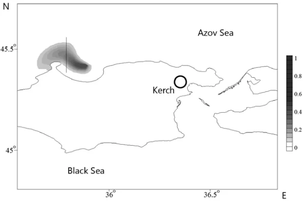
Simulation of the pollution distribution from a permanent unit power source was carried out at different wind effect. The software code provides a reference source both on the sea surface QS =1 and at the bottomQB =−1. Now we are to
consider the case QB =−1 in Kazantip Bay under the eastern wind. Under such wind effect an intense "airing" of the Bay takes place, and the admixture distributes to the north-west (Fig. 6). Under assimilation as the measurement data the information taken from the periphery of the contamination area (to the left of the vertical line) is used. Fig. 6, 7 show the scale of values of the concentration field, normalized to the respective maximum values.
PHYSICAL OCEANOGRAPHY NO. 2 (2015) 75
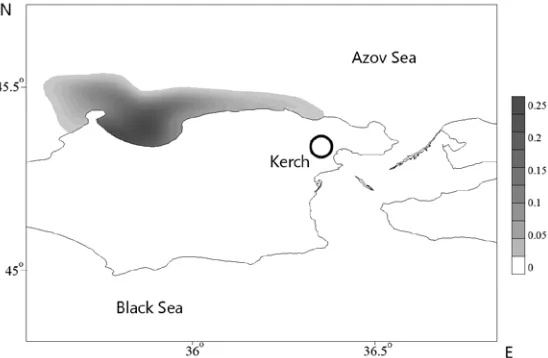
Fig. 7. Influence function (adjoint problem solution)
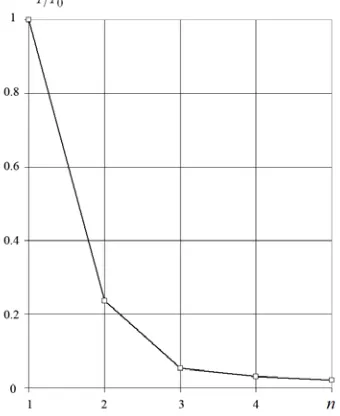
Рис. 8. The fall of the normalized value of the forecast quality functional depends on the number of iterations n at a constant power sourceQB
As a result of the adjoint problem solution (10) – (12) under the first iteration we have the distribution C* at the instant of time t=0 (Fig. 7), featuring the
forecast discrepancy influence on the power
Q
B in the point(
x0,y0)
. In the processof iterations (Fig. 8) the fall of the normalized value of the forecast quality functional takes place and the known value QBrestores. Results of the numeric
of information assimilated. In case of assimilation of all the simulated field information at a finite time to reach the minimum of a functional one iteration is required. The greatest information value the points situated closer to the source of pollution possess.
The article [4] demonstrates that for the time variable of the source power
( )
tQ information about the entire concentration field at a finite time is necessary.
Taking into consideration the possibility of time and space measurement data distribution, it can also be argued that for a more accurate identification ofQ
( )
t , it is necessary to have the point of measurement in the area adjacent to the source of pollution.Conclusion. In general, the performed numerical experiments showed the reliable operation of the variation algorithm of power source identification in relation to the model of passive admixture transport in the Azov Sea. The results can be used to solve various problems of ecological orientation in the study of the impact of anthropogenic pollution sources in the waters of the Azov and Black Sea.
REFERENCES
1. Ivanov, V.A., Fomin, V.V., 2008, “Matematicheskoe modelirovanie dinamicheskikh protsessov v zone more – susha [Mathematic modeling of the dynamic processes in the zone sea-land]”, Sevastopol, ECOSI-Gidrofizika, 363 p. (in Russian).
2. Kochergin, S.V., Kochergin, V.S. & Fomin, V.V., 2012, “Opredelenie kontsentratsii passivnoy primesi v Azovskom more na osnove resheniya serii sopryazhennykh zadach [Determination of the passive admixture concentration in the Azov Sea based on the solution of the adjoint problems]”, Ekologicheskaya bezopasnost' pribrezhnoy i shel'fovoy zon i kompleksnoe ispol'zovanie resursov shel'fa, iss. 26, vol. 2, pp. 112-118 (in Russian).
3. Marchuk, G.I., Penenko, V.V., 1978, “Application of optimization methods to the problem of mathematical simulation of atmospheric processes and environment”, Modeling and Optimization of Complex Systems, Ed. G.I. Marchuk, Proc. оf the IFIP-TC7 Working conf., New York, Springer, pp. 240-252.
4. Kochergin, V.S., Kochergin, S.V., 2010, “Ispol'zovanie variatsionnykh printsipov i resheniya sopryazhennoy zadachi pri identifikatsii vkhodnykh parametrov modeli perenosa passivnoy primesi [Application of adjoint problem principles and solution during the identification of the passive admixture transport model input parameters]”, Ekologicheskaya bezopasnost' pribrezhnoy i shel'fovoy zon i kompleksnoe ispol'zovanie resursov shel'fa, iss. 22, pp. 240-244 (in Russian).