THERMO-GEOMETRIC PARAMETER EFFECTS ON CONVECTIVELY
COOLED INHOMOGENEOUS RECTANGULAR FIN
Ernest Léontin Lemoubou
a, Hervé Thierry Tagne Kamdem
a,*, Jean Roger Bogning
ba
Department of Physics/Faculty of Sciences, University of Dschang, P.O. Box 67,Dschang, Cameroon
b
Department of Physics, H.T.T.C. Bambili, University of Bamenda, Bamenda , Cameroon
A
BSTRACTNumerical experiments involving heat transfer were performed to analyze the influence of both fin thermo-geometric parameter and cooling boundary conditions on the temperature distribution and the efficiency of convective cooled inhomogeneous rectangular fin. The inhomogeneity of the fin is due to both temperature dependent thermal conductivity and convection heat coefficients. The analysis was facilitated by the use of the differential transformation method, which can solve nonlinear differential equation. A specific application is first made for temperature/efficiency homogeneous fin predictions and the results are in excellent agreement with standard exact results. Predictions of inhomogeneous fin temperature and efficiency for three different convection conditions are then performed. The thermo-geometric parameter range for numerical experiments was from 0.0 to 1.0. The results reveal that the thermo-geometric parameter plays a great role in the amount of fin temperature distribution and efficiency. The temperature distribution within the fin is low for high thermo-geometric parameter value and increases rapidly for large values of this parameter. For geometric parameter greater than 0.3, the use of rectangular fin will be optimal for heated or cooled process having heat transfer coefficient increased with increased temperature as generally accounted in laminar or turbulent natural convection. On the other hand, the efficiency of the inhomogeneous fin does not depend on cooling conditions when the thermo-geometric parameter is less than 0.3.
Keywords: Conduction, cooling conditions, Differential transformation method, Heat transfer, Rectangular fins.
1. INTRODUCTION
There are *many concepts of cooling electrical motors and generators. If the machine can be cooled more efficiently, the amount of copper used can decrease and therefore the price of material needed for the machine may also reduce, and the machine will be more cost effective. For this reason, one way to meet these challenges and trade-offs is through the engineering of fin geometry and fin density of heat transfer devices such as heat exchangers and cold plates (Wen and Yeh, 2015; Pal and Majumder, 2016). The fins are therefore presented everywhere in engineering and have a major role in the refrigeration process, air conditioning, and aerospace applications (Kraus et al., 2001; Boonloi and Jedasadaratanachai, 2014). In order to predict the thermal heat behavior of fins, developments of accurate tools for the analysis of heat transfer are required.
Several analytical and semi-analytical methods have been proposed to solve the heat conduction problem through inhomogeneous fins including power series (Díez et al., 2009), the Adomian decomposition (Bhowmik et al., 2013); the homotopy (Moitsheki et al., 2015), the variation iterative and the differential transform methods (Joneidi et al., 2009). However, the differential transformation method (DTM) is well-known as an approximate analytical solution which provides more accurate results compared to other techniques such as the Adomian decomposition method and the variation iterative method (Salehi et al., 2012). The DTM method is based on the Taylor series expansion and constructs an analytical solution in a polynomial form by using the iterative procedure. This method can be used for solving analytically and numerically, linear and nonlinear system of ordinary
* Corresponding author Email:[email protected]
differential equation. It has been used by many authors for heat conduction predictions through fins with various boundary conditions (Joneidi et al., 2009; Kundu and Lee, 2012; Torabi and Aziz, 2012). These previous studies mostly investigated the ability of the DTM to deal with nonlinear heat conduction problems.
In this work, the influence of both fin thermo-geometric parameter and cooling boundary conditions on inhomogeneous fin efficiency and temperature distribution is investigated using a comprehensible DTM formulation. In the development of the method, the heat conduction through inhomogeneous rectangular fin subjected to convective boundary conditions is written in term of fin profile. The inhomogeneity of the fin is due to the variable thermal conductivity. Three convection conditions corresponding to cooling with constant convection coefficient, growing and decaying convection coefficient with fin temperature will be considered.
2. DESCRIPTION OF THE PROBLEM
The problem consists of straight rectangular fin with the length (L), the height (b) and the thickness (w) as shown in Fig. 1. The fin surface temperature is maintained lower than the surrounding air to be cooled. The system allows a fast rise of temperature and maintains it depending to the operation. This is done through the cooled fluid that generally can be water, air, oil, etc. For the mathematical formulation developed here, the one-dimensional heat conduction in the rectangular fin under steady state conditions is assumed. Moreover, the temperature at the basic surface is considered constant and the flux is assumed to be zero at the bottom.
Frontiers in Heat and Mass Transfer
Fig. 1 Sketch diagram for the longitudinal fin with rectangular profile The energy balance based on the Fourier and Newton laws for longitudinal fins as a function fin profile can be written as
( ) ( ) ( ) − ℎ( )( ( ) − ) = 0 , 0 ≤ ≤ (1)
where the characteristic profile can be given by (Kraus et al., 2001)
p(x) =w 2
x b
( ʋ )( ʋ )
(2)
For rectangular profile the parameter ʋ = 1 2⁄ . In Eq. (1), the thermal conductivity of the fin material is a linear function of the temperature
= [1 +( − )] (3)
where is the thermal conductivity at ambient temperature and is the thermal expansion coefficient. The convection coefficient is also dependent on the temperature as (Bhowmik et al., 2013)
ℎ( ) = ℎ −
− (4)
where ℎ is the heat transfer coefficient at ambient temperature and the real specifiying the type of cooling mode may vary for practical applications between -3 and 3 (Kraus et al., 2001). It should be noted that the heat transfer coefficient is constant for n = 0, whereas this coefficient growth with the fin temperature for laminar natural convection, turbulent natural convection, nucleate boiling and radiation. The heat transfer coefficient decays with fin temperature for laminar film boiling or condensation. In order to analyse these three classes of convection conditions, cases with n = -1, 0 and 1, should be considered in this work. The boundary conditions associated to the problem are
⌋ = (5 )
= 0 (5 )
The fin efficiency can be evaluated as the ratio of the heat transfer rate, at the fin base to its ideal transfer rate, if the entire fin were at the same temperature as its base
= =∫ ( − )
( − ) (6)
where U is the perimeter of the convective heat transfer surface. Considering the following dimensionless parameters
= ( ) −
− , = , =( − ) ( 7)
The parameter is the gradient of the thermal conductivity. The problem formulation in dimensionless variables is
(1 + ) ()
− ℎ = 0 , 0 ≤≤ 1 (8)
⌋ = 1 (9 )
= 0 (9 )
with the fin characteristic profile
() = 2()
( ʋ )( ʋ ) (10)
Considering the dimensionless variable, the fin efficiency becomes = ∫ () (11)
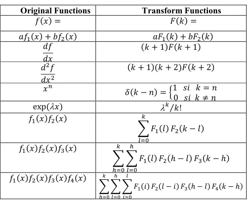
Table 1 One-dimensional DTM fundamental operations
Original Functions Transform Functions
( ) = ( ) = ( ) + ( ) ( ) + ( )
( + 1) ( + 1)
( + 1)( + 2) ( + 2)
( − ) = 1 = 0 ≠
exp ( ) ⁄ !
( ) ( )
( ) ( − )
( ) ( ) ( )
( ) (ℎ − ) ( − ℎ)
( ) ( ) ( ) ( )
( ) ( − ) (ℎ − ) ( − ℎ)
3. DIFFERENTIAL TRANSFORM SOLUTION
3.1 Basic Concept of the Differential Transform Method Let f(x) be the analytic function in a certain domain D and let be a point of this domain. The Taylor series representation of this function is given by (Kundu and Lee, 2012; Torabi and Aziz, 2012)
( ) = ( −( ) ) ( ) !
( )
(12)
The differential transform of the original function f(x) can be expressed as follow (Arslanturk, 2005)
( ) = ( ) !
( )
(13)
variable such that ∈ [0, ]. The inverse transformation of the equation (13) is given by the following formula (Joneidi, 2009)
( ) = ( − ) ( )
( ) !
( )
∀ ∈ (14)
Comparing expressions (13) and (14), it is found that
( ) = − ( ) (15)
Mathematical operations performed by the DTM are presented in table1. The DTM represents a Taylor series of the original function f(x). In this work all expansions are taken around the origin xi = 0 and the
convergence is ensured by choosing the value H = 1and the limit number of discrete coefficient equal to N (Kundu and Lee, 2012; Torabi and Aziz, 2012).
3.2Application of DTM to conduction heat transfer equation Considering the differential transformations of table1, the transformation of the Eq. (8) leads to
(ℎ − + 1)( − ℎ + 1) ( )(ℎ − + 1)( − ℎ + 1)
+ ( − ℎ + 2)( − ℎ + 1) ( )(ℎ − )(
− ℎ + 2) + ( + 1) ( + 1)
+ ( − + 1)( ) ( − + 1)
−ℎ
2
… ( ) ( − ) …( − )
+ ( − + 2) ( )( − + 2)
= 0 (16)
For a rectangular profile as described in Fig. 1, the profile function of the system is constant and independent to the position. The transform profile is ( ) = ( ) 2⁄ (17)
Introducing Eq. (17) in Eq. (16) leads to
( − + 1)( − + 2)( )( − + 2)
+ ( + 1)( − + 1)( + 1)( − + 1)
−Y … ( ) ( − ) …( − )
+ ( + 1)( + 2)( + 2) = 0 (18)
where = 2 ℎ ⁄ is the fin thermo-geometric characteristic parameter. The boundary conditions Eq. (9) become, respectively
( ) = 1 (19 )
(1) = 0 (19 )
In fact, knowing that the solution of the problem arises in the form (15), the second discrete value is zero (1) can be deduced from the second boundary condition. Then, other values of discrete coefficients are deduced from the first discrete value(0).
3.3 Cases Studies
In developing the methods of solution, three cooling conditions will be investigated: heat transfer coefficient may decay with the temperature, constant or growing with the temperature. For the first problem, the heat transfer coefficient is assumed to decrease as temperature increases, which correspond to = −1 in Eq. (4). In such case, Eq. (18) reduces to
( + 2) = −1
( + 1)( + 2) [( − + 1)( − + 2)( )( − + 2)
+ ( + 1)( − + 1)( + 1)( − + 1)]
−Y ( ) (20)
Then, the following discrete coefficients are obtained
(2) = Y
2(1 + ) , (4) = −
Y
8(1 + )
(6) =
Y
16(1 + )
(8) = −
Y
32(1 + ) … , ℎ =(0)
(2 + 1) = 0, = 1, 2, 3, …
Therefore, the temperature distribution within the fin is approximated in Taylor series of dimensionless coordinate as
() = (21)
with
= Y
2(1 + ), = −
Y
8(1 + )
=
Y
16(1 + ) , = −
Y
32(1 + )
and where the constant is determined by using the discrete coefficients together with the first boundary condition, Eq. (19a), as
= 1 (22)
= Y (23)
with
= , = 1
6(1 + ), = −40(1 + ) ,
=
112(1 + ) , = −
288(1 + )
The second problem consists of a rectangular fin cooling by air having a constant heat transfer coefficient that is = 0 in the Eq. (4). Then, Eq. (18) reduces to
( + 2) = −1
( + 1)( + 2) [( − + 1)( − + 2)( )( − + 2)
+ ( + 1)( − + 1)( + 1)( − + 1)]
−Y ( ) (24)
Hence, the following discrete coefficients can be deduced
(2) = Y
2(1 + ), (4) = −
(2 − 1)Y
24(1 + )
(6) = (2 − 1)(14 − 1)Y
720(1 + )
(8)
= − (2 − 1)[(14 − 1)(27 − 1) + 35 (2 − 1)]Y
40320(1 + )
(2 + 1) = 0 = 0, 1, 2, 3, ….
Substituting these values of the discrete coefficients in Eq. (15), the dimensionless temperature distribution within the fin is approximated in Taylor series given by Eq. (21) where
= Y
2(1 + ), = −
(2 − 1)Y
24(1 + )
= (2 − 1)(14 − 1)Y
720(1 + )
= − (2 − 1)[(14 − 1)(27 − 1) + 35 (2 − 1)]Y
40320(1 + )
and the coefficient is calculated with the same procedure as previously based on Eq. (22). The efficiency is expressed in Taylor series of the thermo-geometric parameter given by Eq. (23) with the following coefficients
= , =
6(1 + ), = −
(2 − 1) 120(1 + )
= (2 − 1)(14 − 1) 5040(1 + )
= − (2 − 1)[(14 − 1)(27 − 1) + 35 (2 − 1)] 362880(1 + )
In the last problem studied, the heat transfer coefficient of the cooling fluid increased with increased fin temperature par setting = 1 in Eq. (4). Therefore, Eq. (18) becomes
( + 2) = −1
( + 1)( + 2) [( − + 1)( − + 2)( )( − + 2)
+ ( + 1)( − + 1)( + 1)( − + 1)]
−Y ( ) ( − ) (27)
The following discrete coefficients can be deduced
(2) = Y
2(1 + ), (4) =
(2 − )Y
24(1 + )
(6) = [6(1 + ) − (2 − )(13 − 2)]Y
720(1 + )
(8) = ( + )Y
40320(1 + ) , (2 + 1) = 0 = 0,1,2,3, ….
where
= [6(1 + ) − (2 − )(13 − 2)](2 − 26 )
= (2 − )[30(1 + ) − 35 (2 − )]
(2 + 1) = 0 = 0, 1, 2, 3, ….
The dimensionless temperature distribution within the fin is expressed in Taylor series of Eq. (21) where
= Y
2(1 + ), =
(2 − )Y
24(1 + )
= [6(1 + ) − (2 − )(13 − 2)]Y
720(1 + )
= ( + )Y
40320(1 + )
Before substituting in the temperature solution Eq. (21) it is convenient to apply the same treatment based on Eq. (22) to derive the unknown discrete coefficient . The fin efficiency for this case can also approximated in Taylor series given by Eq. (23), where
=
6(1 + ), =
(2 − ) 120(1 + )
= [6(1 + ) − (2 − )(13 − 2)] 5040(1 + )
= − ( + )
362880(1 + )
3. RESULTS AND DISCUSSION
0 0.1 0.2 0.3 0.4 0.5 0.6 0.7 0.8 0.9 1 0.7
0.75 0.8 0.85 0.9 0.95 1
= 0.0 = 0.4 = 0.8
n = 1
0 0.1 0.2 0.3 0.4 0.5 0.6 0.7 0.8 0.9 1
0.65 0.7 0.75 0.8 0.85 0.9 0.95 1
= 0.0
= 0.4
= 0.8
n = 0
0 0.1 0.2 0.3 0.4 0.5 0.6 0.7 0.8 0.9 1 0.5
0.55 0.6 0.65 0.7 0.75 0.8 0.85 0.9 0.95 1
= 0.0 = 0.4 = 0.8
n = -1
0 0.1 0.2 0.3 0.4 0.5 0.6 0.7 0.8 0.9 1 0.65
0.7 0.75 0.8 0.85 0.9 0.95 1
DTM predictions Exact results
n = 0
n = 1
0 0.1 0.2 0.3 0.4 0.5 0.6 0.7 0.8 0.9 1
0.5 0.55 0.6 0.65 0.7 0.75 0.8 0.85 0.9 0.95 1
DTM predictions
Exact results n = 0
n = -1
In Figs. 2 and 3 an excellent accuracy can be seen between DTM temperature and efficiency predictions and exact results for the two convection cooling conditions. This shows that the DTM is an efficient tool for the analysis of heat conduction problem through fin. Still referring to Figs. 2 and 3, a significant difference between cooling with a constant heat transfer coefficient and aheat transfer decreased with increased temperature is seen to be the temperature depend heat transfer coefficient effect on the cooling of the rectangular fin.
Fig. 2 Comparison of DTM and exact solution for the fin temperature when ψ = 1 and β = 0 for two convection conditions: n = -1 and n = 0
Fig. 3 Rectangular fin efficiency versus thermo-geometric parameter for the constant thermal conductivity and for two convection conditions: n = -1 and n = 0
The temperature profile with convection condition using constant heat transfer coefficient is much higher than for the convection condition with heat transfer decreased with increased fin temperature. Therefore, rectangular fin for cooling process will be more efficient for cooling process having a heat transfer decreased with increased fin temperature as appearing in Fig. 3, which also compared rectangular efficiency for the two cooling conditions considered.
The DTM is then used to investigate the effect of temperature dependent thermal conductivity and/or temperature depend heat transfer coefficient effects on the cooling of the rectangular fin. It should be noted, that the thermal conductivity variation with the temperature led to a nonlinear equation of conduction in the fin which is difficult to solve analytically. Also, the heat transfer coefficient increased with increased fin temperature yield a governing equation of conduction through the fin difficult to solve analytically even when for constant
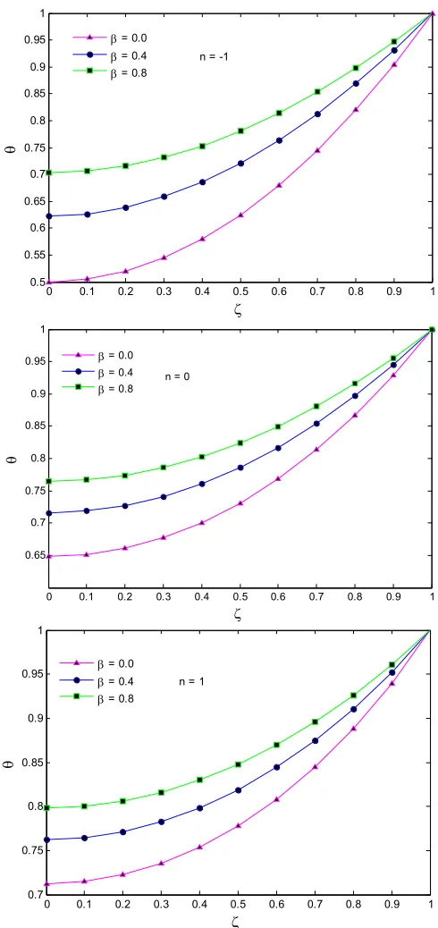
thermal conductivity. Comparisons of predicted temperature profiles for three gradients of the thermal conductivity and three cooling conditions are shown in Figs. 4 when the fin thermo-geometric characteristic parameter is equal to one.
Fig. 4 Temperature for variable thermal conductivity for various cooling conditions n = {-1, 0, 1} when the fin thermo-geometric parameter Ψ = 1
0 0.1 0.2 0.3 0.4 0.5 0.6 0.7 0.8 0.9 1 0.7
0.75 0.8 0.85 0.9 0.95 1
n = -1 n = 0 n = 1
= 0.8
0 0.1 0.2 0.3 0.4 0.5 0.6 0.7 0.8 0.9 1 0.65
0.7 0.75 0.8 0.85 0.9 0.95 1
n = -1 n = 0 n = 1
= 0.4
0 0.1 0.2 0.3 0.4 0.5 0.6 0.7 0.8 0.9 1 0.5
0.55 0.6 0.65 0.7 0.75 0.8 0.85 0.9 0.95 1
n = -1 n = 0 n = 1
= 0.0
0 0.1 0.2 0.3 0.4 0.5 0.6 0.7 0.8 0.9 1
0.75 0.8 0.85 0.9 0.95 1
= 0.2 = 0.6 = 1.0 n = 1
0 0.1 0.2 0.3 0.4 0.5 0.6 0.7 0.8 0.9 1
0.7 0.75 0.8 0.85 0.9 0.95 1
= 0.2 = 0.6 = 1.0 n = 0
0 0.1 0.2 0.3 0.4 0.5 0.6 0.7 0.8 0.9 1 0.65
0.7 0.75 0.8 0.85 0.9 0.95 1
= 0.2 = 0.6 = 1.0 n = -1
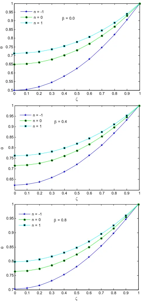
of temperature profile for cooling condition with heat transfer coefficient increased as the fin temperature increased when compared with cooling condition with constant heat transfer coefficient for each gradient of the thermal conductivity considered. These behaviors are much more appreciable in Figs. 5, which illustrates the effect of different thermal conductivity gradient of the fin temperature subject of various cooling conditions when the fin thermo-geometric characteristic parameter is equal to one. It is noted in Figs. 5 that, for a constant thermal conductivity, the difference between cooling with constant heat transfer coefficient and heat transfer coefficient increased with increased fin temperature is insignificant, whereas there are considerable differences between the three cooling conditions when the thermo-geometric characteristic parameter is different from zero.
Fig. 5 Comparison of temperature for different gradient of the thermal conductivity and for various cooling conditions when the thermo-geometric parameter Ψ = 1
.
Fig. 6 Fin temperature profile for different convective conditions and for the thermo geometric parameter Ψ = {0.2, 0.8, 1.0} when the thermal conductivity gradient β = 0.5
0 0.1 0.2 0.3 0.4 0.5 0.6 0.7 0.8 0.9 1 0.65
0.7 0.75 0.8 0.85 0.9 0.95 1
n = -1 n = 0 n = 1 Convection conditions
noted that the temperature is higher when the heat transfer coefficient decreased with increased temperature, whereas it is lower for the heat transfer coefficient increased with increased temperature.
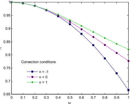
Fig. 7 Fin efficiency versus thermo-geometric parameter for three convection conditions for the constant conductivity
Accordingly, this is well shown in Fig. 7 where the change of fin efficiency with thermo-geometric parameter for the thermal conductivity gradient is higher when the heat transfer coefficient increased with increased temperature whereas it is lower when the heat transfer coefficient decreased with increased temperature. Also, it can be observed in Fig. 7 that the fin efficiency decreases with increasing values of the thermo-geometric fin parameter. For rectangular fin thermo-geometric parameter less than 0.3, cooling conditions have identical effect on the rectangular fin, while for its value greater than 0.3 the fin efficiency therefore depends on the nature of the heat convection cooling condition. The cooling condition with the heat transfer coefficient increased with increased temperature led to higher efficiency compared to the two other conditions.
4. CONCLUSIONS
In this study, a one-dimensional differential transformation method is applied to solve nonlinear differential equation arising in stationary heat conduction in convective straight rectangular fin with temperature-dependent thermal conductivity. Three different cooling convection conditions have been considered: constant heat transfer coefficient, heat transfer increased and decreased with the fin temperature. The DTM applied to the heat conduction equation in the fin as its profile yield expression suitable for the numerical analysis. The results obtained are summarized as follows:
o An excellent agreement is observed between DTM temperature and efficiency predictions and exact results for homogeneous rectangular fin.
o The temperature distribution and efficiency of homogeneous and inhomogeneous fin can be accurately described by a Taylor series of order eight.
o The temperature distribution within the fin depends on both the fin thermo-geometric parameter and cooling boundary condition.
o The fin efficiency decreased with increasing thermo-geometric parameter.
o The fin efficiency is lower for large value of the thermo-geometric parameter, whereas it is independent of cooling condition for of the thermo-geometric parameter less than 0.3.
The effect of the cooling condition is prominent for the heat transfer coefficient increasing with increasing temperature as generally accounted laminar or turbulent natural convection.
NOMENCLATURE
b height of the fin (m)
h heat convectivity coefficient ( ∙ ∙ )
K thermal conductivity heat coefficient ( ∙ ∙ )
q heat flux (W/m2)
T temperature ( K )
U section perimeter (m)
x coordinate (m)
p profile function
P profile transform function
W thickness of the fin (m)
Greek Symbols
dimensionless temperature thermal expansion coefficient ( ) dimensionless temperature
dimensionless temperature transform function fin efficiency
parameter of the profile function Ψ thermo-geometric parameter dimensionless coordinate
Subscripts
b fin base
i ideal parameter
∞ ambient environment
REFERENCES
Arslanturk, C., 2005, "A Decomposition Method for Fin Efficiency of Convective Straight Fins with Temperature-Dependent Thermal Conductivity," International Communication of Heat Mass Transfer,
32, 831-841.
http://dx.doi.org/10.1016/j.icheatmasstransfer.2004.10.006
Bhowmik, A., Singla, R. K., Roy, P. K., Prasad, D. K., Das, R., and Repaka R., 2013, "Predicting Geometry of Rectangular and Hyperbolic Fin Profiles with Temperature-Dependent Thermal Properties using Decomposition and Evolutionary Methods," Energy Conversion and Management, 74, 535-547.
http://dx.doi.org/10.1016/j.enconman.2013.07.025
Boonloi, A., and Jedasadaratanachai, W., 2014, "3D Numerical Analysis on Flow Configurations and Heat Transfer Characteristics for Fin-and-Oval-Tube Heat Exchanger with V-Downstream Delta Winglet Vortex Generators," Frontiers in Heat and Mass Transfer, 5, 013019.
http://dx.doi.org/10.5098/hmt.5.19
Díez L. I., Campo A., and Cortés C., 2009, "Quick Design of Truncated Pin Fins of Hyperbolic Profile for Heat-Sink Applications by using Shortened Power Series," Applied Thermal Engineering, 29, 815-821.
http://dx.doi.org/10.1016/j.applthermaleng.2008.04.001
Joneidi A. A., Ganji D. D., and Babaelahi M., 2009, "Differential Transformation Method to Determine Fin Efficiency of Convective Straight Fins with Temperature Dependent Thermal Conductivity,"
International Journal of Heat and Mass Transfer, 36, 757-762.
http://dx.doi.org/10.1016/j.icheatmasstransfer.2009.03.020
Kundu, B., and Lee, K. -S., 2012, "Analytic Solution for Heat Transfer of Wet Fins on Account of all Nonlinearity Effects," Energy, 41, 354-367.
http://dx.doi.org/10.1016/j.energy.2012.03.004
Moitsheki, R. J., Rashidi, M. M., Basiriparsa, A., and Mortezaei, A, 2015, "Analytical Solution and Numerical Simulation for One-Dimensional Steady Nonlinear Heat Conduction in a Longitudinal Radial Fin with Various Profiles," Heat Transfer-Asian Research,
44(1), 20-38.
http://dx.doi.org/10.1002/htj.21104
Pal, D. C., and Majumder, A., 2016, "Numerical Study of Fin-Tube Type Heat Exchanger with Delta Winglets," Fontiers in Heat and Mass Transfer, 7, 013001.
http://dx.doi.org/10.5098/hmt.7.1
Salehi, P., Yaghoobi, H., and Torabi, M., 2012, "Application of the Differential Transformation Method and Variational Iteration Method
to Large Deformation of Cantilever Beams Under Point Load," Journal of Mechanical Science and Technology, 26(9), 2879-2887.
http://dx.doi.org/10.1007/s12206-012-0730-y
Torabi, M., and Aziz, A., 2012, "Thermal Performance and Efficiency of Convective-Radiative T-Shaped Fins with Temperature Dependent Thermal Conductivity, Heat Transfer Coefficient and Surface Emissivity," International Communication of Heat Mass Transfer, 39, 1018-1029.
http://dx.doi.org/10.1016/j.icheatmasstransfer.2012.07.007
Wen M.-Y., and Yeh C. H., 2015, "Natural Convective Performance of Perforated Heat Sinks with Circular Pin Fins," Heat Mass Transfer, 51, 1383-1392.