Structural orientation optimization of the pole mount support of a solar panel for wind load by using CFD analysis

(1)

Int. J. Adv. Res. Sci. Technol. Volum e 3, Issue4, 2014, pp.224-231

International Journal of Advanced Research in

Science and Technology

journal homepage: w w w .ijarst.com

IS S N 2319 – 1783 (Print)

IS S N 2320 – 1126 (Online)

Structural orientation optimization of the pole mount support of a solar panel for

wind load by using CFD analysis

K. V. Siva Apparao, T. Prak ash Lazarus and I. Satyanarayana

Department of Mechanical, Chaitanya College of Engineering, Visakhapatnam, India.

*Corresponding Author’s Email: [email protected]

A R T I C L E I N F O A B S T R A C T

Article history: Received Accepted Available online

12 Nov. 2014 17 Dec. 2014 27 Dec. 2014

In the recent years the electricity generation price has been increasing rapidly. So world is in search for technologies where renewable energies are used for electricity production. This can reduce the prices on the electricity that is generated. Renewable energies are nothing but the energy source that is naturally regenerated such as wind, tides, sunlight, rain, waves etc. Out of these, solar energy (energy from sunlight) can be easily collected. In the current study, CFD simulations were carried out to estimate the wind Effect for various angles. Simulations were carried out for 55m/s, 70m/s at different inclination (θ) angles like 28,30,32,34 For slandered wind direction. It was observed that at a specific distance between two sets of panels and the lift, drag coefficient for the panels reaches a minimum. Another investigation was performed to determine the maximum strength of the solar panel supporting stretcher for effect of aerodynamic pressure.

Keywords: Catia V5,

ANSYS (Structural analysis), ANSYS (CFD).

Introduction:

The use of solar panel technology has recently increased in both domestic and industrial applications. This increased usage has been driven by the increasing financial cost of electric power, and the public desire to produce a greater proportion of energy from renewable resources and also to offset the power costs during pick periods. Based on their applications these panels are manufactured in different shapes and sizes. In industrial applications set of panels are considered in arrayed configuration (figure 1). Each set includes 3*4 or 2*3 panels close to each other with a small gap between them.

For ease of maintenance and air ventilation purposes the panels are installed 2 to 5 feet above the ground. Given the large surface area the aerodynamic forces acting simultaneously on these modules could cause serious mechanical problems to the systems. Therefore, a good understanding of the wind flow and its interaction with the arrayed sets of panels is of interest to minimize the potential damages.

In the current study, computational fluid dynamics simulations are carried out to estimate the wind loads on stand-alone and arrayed sets of solar panels to study the effects of various wind directions (θ) and inclination angles (φ). Simulations are performed for arrayed sets of solar panels to investigate the sheltering effects of

one set on another. Numerical simulations are performed on three sets of solar panels in a tandem configuration for three azimuthal wind directions. An important reduction in drag force is observed on the second and third sets of solar panels.

One of the widely commercialized solar energy technologies is the photovoltaic (PV) solar cells that convert the sunlight directly into electricity. The solar cells are made of semiconductors materials such as Silicon or Cadmium Telluride (CdTe). Sunlight contains energy particles called photons. When light from the sun incidents on a solar cell, the photons are absorbed by the semiconductor material. The absorbed photons knock electrons (e-) out of their atoms in the semiconductor creating a hole (h+). The design of the semiconductor diode ensures that the released electrons move in a single direction and produces electricity . Sets of solar cells are combined to make a solar panel. They are installed by fastening them to a framework or support structure as standalone units or as an array of PV units. A standalone solar PV structure may also comprise of several individual panels arrayed as a single structure.

(2)

Int. J. Adv. Res. Sci. Technol. Volum e 3, Issue4, 2014, pp.224-231 on its two surfaces. The surfaces of the solar panels

thereby experience the drag force in the direction of the wind flow and lift force in the direction perpendicular to the flow. These forces produce the torque. The drag force is expressed as

Drag Coefficient Cd =

Lift Coefficient Cl =

Where, ρ, , A, Cd, Cl refers to air density, wind velocity, projected area, coefficients of lift and drag, respectively. Torque is expressed as the product of force and the displacement vector from the point where the force is applied. These forces are depicted schematically in Figure 1-1. In case of strong winds these forces and the resulting torque could damage the solar panel structure. An example of such damage is shown in Figure 1-2 where a severe typhoon damaged the solar collectors in Taiwan [5]. Although there are practical limits to the protection of solar panels in extreme wind situations, nonetheless proper understanding of the wind phenomenon at the site can help prevent solar panel damages by more frequent wind gusts.

Wind engineering researches developed from the need to protect high-rise, typically slender structures from wind damage. The investigations conducted on the World Trade Center are one of the early projects that defined wind engineering studies [6, 7]. Wind codes have been developed as receptacles for the knowledge obtained from wind engineering. Investigations of wind effect on low-rise structures are now common [8-10] and they have provided valuable data into various wind codes. However, existing wind codes do not yet have a guide for solar panels. The National Building Code of Canada states that structures should be designed so that they can withstand pressures and suction from the strongest wind generated in that area based on wind statistics. Engineers can determine the wind loading using any of the three methods proposed by the American Society of Civil Engineers in the ASCE 7-05 manual [11]. The three methods are known as the simplified method, analytical method and wind tunnel method. The simplified ASCE Method is not suitable to estimate the loads on solar panels because they are not enclosed structures. Eligible structures for the analytical method should not be on a site for which wake buffeting will be considered [12]. Solar Panels do not meet the requirements for both the simplified and analytical methods. This is because solar panels are known to be susceptible to vortex shedding and wake buffeting [13, 14]. Therefore, studies of wind effect on solar panels are conducted using wind tunnel method or Computational Fluid Dynamics (CFD). However, the accuracy of CFD modeling relies on its validation with the experimental data. The common techniques used in wind tunnel studies of structures are flow

visualizations, hot-wire anemometry, local pressure taps and high frequency force balance [15].

Specification of the Problem:

Previous studies showed that solar plate must be placed at some inclination with respect to ground, so that when the wind strikes the inclined solar panel, then it flows around the panel and so produces unequal pressure on both of its surfaces. Due to this the solar panels undergoes drag in wind flow direction and lift force in perpendicular direction to wind flow. [ i ]

Drag Coefficient: In fluid dynamics, drag coefficient is a dimensionless quantity. It is used to quantify the drag or resistance of an object in a fluid environment (water or air). The low drag coefficient indicates that it is safe and have less hydrodynamic drag. It is always related to a surface area. Drag coefficient is not a constant number. It varies as the function of speed. [ ii ]

Drag Coefficient Cd =

Where F= Drag force,

= Density of air,

V = Velocity of wind,

A = Projected area

Lift Coefficient: Lift coefficient is also a dimensionless number similar to drag coefficient. Generally it relates to the lift generated by a lifting body to the density of air of water around the body, velocity and a reference area. Lift coefficient is a function of the angle of the body to the flow. [iii ]

Lift Coefficient Cl =

Where L = Lift force,

= Density of air,

V = Velocity of wind,

S = Projected area.

Generally Torque is a product of force and displacement vector from where force is applied. During high winds the solar module structure may get damaged due to the force and the resulting torque.

(3)

One can determine the wind loading three methods. They are analytical method, simplified method and wind tunnel method. These methods are proposed by American society of civil engineers in ASCE 7-05. Analytical method could not be used for solar plates, because for analytical method the structure should not be placed in a site. So this method cannot be used. Other method which is simplified method also cannot be used on solar plates. This is because solar plates are not enclosed structures. So wind studies on the solar plate are conducted used Computational fluid dynamics (CFD) or wind tunnel method.

Nomenclature:

a absorption coefficient Ar Archimedes Number

C linear-anisotropic phase function coefficient Cp specific heat

d distance

CD Coefficient of drag CL Coefficient of lift P pressure

Re Reynolds Number Ra Rayleigh Number t time

T absolute temperature

Tu turbulence intensity in percent u velocity component in the x direction v velocity component in the y direction sv mean fluid velocity

g gravitational acceleration G incident radiation

Gb generation of turbulent kinetic energy that arises due to buoyancy

Gk generation of turbulent kinetic energy the arises due to mean velocity gradients

Gr Grashof number

s Stefan-Boltzmann Constant (5.672 x10-8 W/m2 – K4)

w specific dissipation rate of turbulent kinetic energy, k

e rate of dissipation of kinetic energy u kinematic fluid viscosity

b thermal expansion coefficient ρ mass density

LE Leading edge Na N Not-a-number

NBCC National Building Code of Canada PIV Particle Image Velocimetry

PV Photovoltaic

PVC Polyvinyl chloride SNR Signal-to-noise ratio TE Trailing edge

4.1 CFD analysis on solar plate at inclination angle 28,30,32,34 degrees at a speed of 55m/s:

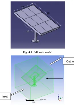
A 3x3 silicon photovoltaic cell is modeled and then analyzed. The modeling is done in CATIA. The 3-D solid modeling is shown in the figure 4.1.Each panel has 40 mm length, 40mm width and 4mm thickness. Now the size of the model is 120 mm length and 120

mm width and 4mm thick. This panel is placed on stainless steel stand and a frame. The size of the frame is 2 mm thick which comes around the solar plate. The PV cell is kept at inclination angle of 28 degrees with respect to ground which is shown in figure 4.1.

This 3D model is later imported to fluent in ANSYS. A box type domain which is called an enclosure is created in geometry editor in fluent and then solar model is kept in that. Now Boolean is created and the target body and tool bodies should be selected. The total model is approximately 150 mm in length, 150 mm in breath and 150 mm in width which is shown in figure 4.2. The boundary conditions are also clearly shown in the figure 4.3.

Fig. 4.1: 3-D solid model

Fig. 4.2: Flow boundary conditions

Later the mesh is applied to the both domain and the whole solar plate and then generated. Here I have applied tetra solid mesh. This is shown in figure 8. Now the boundary types are defined. Every wall of the geometry cannot be used for the same purpose. In this study the air should enter from the positive y direction and should leave from the face opposite to it. Fluent don’t know what user want. So the user should define inlet, outlet and walls. The face through which air starts to flow is selected and then right click to select name selection. Then a popup appears where we need to give the name as inlet. Similarly the outlet face is selected

Out let

Domain

(4)

Int. J. Adv. Res. Sci. Technol. Volum e 3, Issue4, 2014, pp.224-231 and name is given as outlet. Then the remaining four

faces are selected and they are named as walls. In the figure 8 the blue face indicates the inlet; the red face indicates the outlet and white faces indicates walls. Now the mesh is generated and the boundary types are defined properly.

Now we need to double click the setup so that the model is opened in the fluent. I have selected 3D in dimension, double precision in options and series in processing options. Now the fluent is launched. As soon the fluent is launched, we can see that mesh is automatically generated. Now I have clicked on check to check my geometry. Next I have clicked on scale and selected units as mm. Next I have clicked on unit’s button. Then a window is opened where I have selected velocity and units as m/s.

Design Specifications of solar panel:

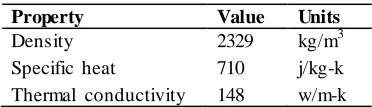
Table: 4.1. Mechanical properties of silicon

Property Value Units

Density 2329 kg/m3

Specific heat 710 j/kg-k

Thermal conductivity 148 w/m-k

4.2 CFD analysis on solar plate at inclination angle 28,30,32,34 degrees with wind speed 55 m/s:

In this case I have done analysis on a solar plate with same dimensions. i.e. 120 mm x 120 mm x 4 mm. This makes inclination angle 28,30,32,34 degrees with ground. The whole analysis is done in the same procedure as explained in section 3.1. Even the boundary physics is same i.e. the inlet and outlet is given to the same faces as above. But the major difference was the boundary conditions. In this case I have taken wind velocity as 55 m/s which is way high than the velocity which was taken in section 4.4 (55 m/s). Due to this some of the values in the boundary conditions change.

Turbulent Kinetic energy (m2/s2) =

Turbulence Dissipation Ratio (m2/s3) = E =

Here

ϑ = 55 m/s

K = 552/10000

= 0.3025 m2/s2

Flow material Density kg/m3

0.09 Constant

µ = 0.001

By substituting these values we get

Turbulence Dissipation Ratio = 0.1844 m2/s

Table: 4.3. Boundary conditions for wind velocity 55 m/s

Velocity Specification method

Components

X-velocity 0 m/s

Y-velocity 55 m/s

Z-velocity 0 m/s

Specification method K- epsilon method Turbulent kinetic energy 0.3025 m2/s2 Turbulent dissipation

ratio

0.1844 m2/s3

Temperature 300K

Plot 5.3.1Drag coefficient when inclination angle is 32oat wind speed 55m/s

Plot.5.3.2 Lift coefficient when inclination angle is 32o at 55m/s

4.3 CFD analysis on solar plate at inclination angle 32 degrees with wind speed 70 m/s:

(5)

Int. J. Adv. Res. Sci. Technol. Volum e 3, Issue4, 2014, pp.224-231 given to the same faces as above. But the major

difference was the boundary conditions. In this case I have taken wind velocity as 70 m/s which is way high than the velocity which was taken in section 4.9 (70 m/s). Due to this some of the values in the boundary conditions change.

Turbulent Kinetic energy (m2/s2) =

Turbulence Dissipation Ratio (m2/s3) = E =

Here

ϑ = 70 m/s

=

K = 702/10000

= 0.49 m2/s2

Flow material Density kg/m3

0.09 Constant

µ = 0.001

By substituting these values we get

Turbulence Dissipation Ratio = (density x 0.09 x 0.3025 x 0.3025)/(50 x 0.001)

= 0.540225 m2/s3

Table.4.4 Boundary conditions for wind velocity 70m/s

Velocity Specification method

Components

X-velocity 0 m/s

Y-velocity 70 m/s

Z-velocity 0 m/s

Specification method K- epsilon method Turbulent kinetic

energy

0.49 m2/s2

Turbulent dissipation ratio

0.5400225 m2/s3

Temperature 300K

Plot.5.5.1Drag coefficient when inclination angle is 32oat wind speed 70m/s

Plot.5.5.2 Lift coefficient when inclination angle is 32oat 70m/s

6.1 CFD analysis results :

Table: 6. 1. Solar panels supporting stretcher results by varying angles with wind speed 55m/s .

S/No Results 28Deg 30Deg 32Deg 34Deg

1 Drag coefficient 0.0004 0.0003 0.00015 0.0003

2 Lift coefficient 0.225 0.28 0.3 0.35

3 static pressure (Pascal) 3.76e03 4.54e03 4.87e03 5.16e03

4 Dynamic pressure (Pascal). 5.02e03 7.87e03 7.3e03 7.5e03

5 Radial velocity at inlet and outlet (m/s) 8.57e01 1.05e02 1.03e02 1.03e02 6 Turbulent kinetic Energy (k) (m2/s2) 8.54e02 8.57e02 8.52e02 10.8e02

(6)

Table: 6. 2.Solar panels supporting stretcher results at an angle 32Deg with wind speed 70m/s .

S/No Results 32deg

1 Drag Coefficient 0.0035

2 Lift Coefficient 0.25

3 Static Pressure (Pascal) 7.89e03

4 Dynamic Pressure (Pascal). 12.1e03

5 Radial Velocity At Inlet And Outlet (M/S) 1.33e02 6 Turbulent Kinetic Energy (K) (M2/S2) 15.4e02

7 Effective Prandtl Number 0.87

S/No Solar panels supporting stretcher Orientation

Drag coefficient

1 28 Deg 0.0004

2 30 Deg 0.0003

3 32 Deg 0.00015

4 34 Deg 0.0003

4.5 Structural analysis of a solar panel pole mounted supporting structure at 32degrss :

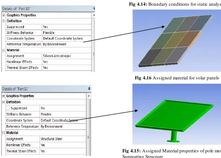
The static analysis of a solar panel pole mounted supporting structure is done in ANSYS, we uploaded .igs file to ansys, the boundary conditions are sh own in fig 4.14 in here Dynamic pressure is applied on front panel supporting structure, the bottom is fixed in all digress of freedom. Material properties of solar panel pole mounted supporting structure are Structural steel shown in fig 4.15 & 4.16.

Fig 4.14: Boundary conditions for static analysis

Fig 4.16 Assigned material for solar panels

(7)

5.6 Structural analysis of a s olar panel pole mounted supporting structure at 32 Deg with a velocity 55m/s.

Input Parameters for (Case-1):- Inlet velocity = 55m/s

Pole mounted structure orientation = 32 Deg Total pressure = 7.3e-3 Mpa

Boundary conditions = Pole mounted supporting structure of bottom is arrested in all DOF

Material Properties of structure = Structural Steel (SS

)

Fig: Dynamic pressure applied on structure

Fig: Equivalent von-mises stress

Fig:- Total deformation

5.7 Structural analysis of a solar panel pole mounted supporting structure at 32 Deg with a velocity 70m/s.

Input Parameters for (Case-2):-

Inlet velocity = 70m/s

Pole mounted structure orientation = 32 Deg

Total pressure = 1.21e-2 Mpa

Boundary conditions = Pole mounted supporting structure of bottom is arrested in all

DOF

Material Properties of structure = Structural Steel (SS)

Fig:- Dynamic pressure applied on structure

Fig:- Solid mesh

Fig:- Equivalent von-mises stress

(8)

Conclusion:

CFD simulations were carried out to estimate the wind Effect on solar panel supporting structure for various angles like 28,30,32,34 for slandered wind direction. Simulations were carried out for 55m/s, 70m/s. we observed that above results turbulent kinetic Energy (k) (m2/s2) Drag coefficient (Cd) are lower at 32 deg angle orientation. So when we are placing solar panel supporting structure at 32 deg is safe for wind loads.

We observed dynamic pressure on solar panel supporting structure 32 deg at a velocity 55m/s,70m/s. obtained pressure is applied on pole supporting structure in static analysis. in this analysis we observed von miss stress and total deformation this are within limits (below yield strength of the material[Structural steel]). So finally we concluded our solar panel pole supporting structure is safe at 32deg for aerodynamic pressure [55,70m/s inlet velocity].

Future Scope:

In present work we complete a rigid pole mount supporting system but in future we change to flexible pole mount supporting system for unidirectional wind load and also as the inner panel gaps are now know to influence wind loading .for the solar panel of this gaps should be investigated in future studies similar to the study conducted by we etal [15] on such gaps for a heliostat.

References:

1. International Energy Outlook 2010, Report # DOE/EIA-0484, US Department of Energy, July 2010.

2. Gray,J. L.(2003).The physics of the solar cell.by A. Luque S. Hegedus.–Chichester: John Wiley & Sons Ltd, 61-112.

3. Ontario Power Authority. Generate Power... and M oney.2011;Availableat:microfit.powerauthority.on.ca/ sites/default/files/news/FITmFITPriceScheduleV2.0.pdf . Last accessed 03/24, 2013.

4. Government of Ontario. Electricity prices are changing.2011;Availableat:

http://www.mei.gov.on.ca/en/pdf/EnergyPlan_EN.pdf. Last accessed 01/21, 2013.

5. Chung, K., Chang, K., & Liu, Y. (2008). Reduction of wind uplift of a solar collector model. Journal of Wind Engineering and Industrial Aerodynamics, 96(8), 1294-1306.

6. Cochran, L. S. (2002, June). Early Days of North American Wind Engineering: An Interview with Professor Cermak about Professor Davenport. In

Proceedings of theEngineering Symposium to Honour Al an G.Davenport for His Forty Years of Contributions. London, Canada: University of Western Ontario.

7. Davenport, A. G. (2002). Past, present and future of wind engineering. Journal of Wind Engineering and Industrial Aerodynamics, 90(12), 1371-1380.

8. Stathopoulos, T. (1984). Wind loads on low-rise buildings: a review of the state of the art. Engineering Structures, 6(2), 119-135.

9. Uematsu, Y., &Isyumov, N. (1999). Wind pressures acting on low-rise buildings. Journal of Wind Engg and Industrial Aerodynamics, 82(1), 1-25.

10. Peterka, J. A., Tan, L., Bienkiewcz, B., &Cermak, J. E. (1987). Mean and peak wind load reduction on heliostats (No. SERI/STR-253-3212). Colorado State Univ., Fort Collins(USA).

11. Structural Engineering Institute. (2006). Minimum design loads for buildings and other structures (Vol. 7, No. 5). American Society of Civil Engineers (ASCE). 12. Hangan, H., & Vickery, B. J. (1999). Buffeting of

two-dimensional bluff bodies .Journal of Wind Engg and Industrial Aerodynamics, 82(1), 173-187

13. Shademan, M . (2010) CFD Simulation of Wind Loading on Solar Panels. (M ESc Dissertation).London, Ont., School of Graduate and Postdoctoral Studies, University of Western Ontario.

14. Kopp, G. A., Surry, D., & Chen, K. (2002). Wind loads on a solar array. Wind and Structures, an International Journal, 5(5), 393-406.

15. we etal ,Rhee, J., Nguyen, C., Grace, M ., & Thu, A. (2011).An effective, low-cost mechanism for direct drag force measurement on solar concentrators. Journal of Wind Engineering and

16. Industrial Aerodynamics, 99(5), 665-669.

About Authors:

K.V. Siva Apparao is a P.G student of Mechanical Department of Chaitanya Engineering College. She done her B.Tech from SCR college of Engineering affiliated to JNTU KAKINADA.

Lazarus T. Prakash M.Tech (Ph.D) is presently Professor & Head of the Department of Mechanical Engineering Department, Chaitanya Engineering College. He has vast experience in the field of teaching. He has guided many projects for B.Tech & M.Tech Students.