* Corresponding author. Tel: +1(812) 461-5385 E-mail: [email protected] (G. Black)
© 2012 Growing Science Ltd. All rights reserved. doi: 10.5267/j.ijiec.2012.03.002
Contents lists available at GrowingScience
International Journal of Industrial Engineering Computations
homepage: www.GrowingScience.com/ijiec
A parallel machine extension to aversion dynamics scheduling
Gary W. Blacka*and Kenneth N. McKayb
a
College of Business, University of Southern Indiana, 8600 University Blvd, Evansville, IN 4771, USA b
Department of Management Sciences, University of Waterloo, 200 University Avenue W, Waterloo, ONT, N2L 3G1, Canada
A R T I C L E I N F O A B S T R A C T
Article history: Received 31 January 2012 Accepted March, 7 2012 Available online 8 March 2012
The aversion dynamics research agenda has incorporated within dispatching heuristics a number of real-world observations involving risk mitigation practices used by real schedulers. One such observation is that schedulers occasionally offload risky jobs from a primary machine to otherwise less desirable machine (older, slower) during periods of peak load to avoid the effects the risky job can have on subsequent jobs. This paper examines this situation within the proportional parallel machine environment. Safety time is used to adjust dispatching priorities of risky jobs to reflect the aversion. The effect of various safety time values on performance is studied. Robust safety time values and/or intervals are identified across a variety of experimental factors related to risk level, percent risky jobs in the job stream, and due date distribution.
© 2012 Growing Science Ltd. All rights reserved
Keywords:
Aversion dynamics Scheduling Risk mitigation Safety time Job re-sequencing
1. Introduction
The gap between scheduling research and practice has inspired an area that has become known as
aversion dynamics (McKay et al. 2000; McKay and Black, 2006). Aversion dynamics is based on
empirical field studies which reveal how production schedulers incorporate aversion to risk within their daily decisions (McKay, et al. 1995; McKay, 1992). For instance, suppose a scheduler delays assigning a sensitive job to a risky machine until such time the risk subsides. An example of this situation is the period of instability shortly after a major machine upgrade or breakdown. Another example is when a scheduler delays assigning a risky job, perhaps a prototype part, to a machine due to the potential effect it can have on subsequent jobs; the prototype part could destabilize the process, machine settings, or possibly damage the machine. When these strategies are incorporated into the
aversion dynamic heuristics, the processing time used for prioritization has been inflated beyond the
nominal time to reflect the risk (a form of surrogate for the risk assessment), thus affecting sequencing decisions.
526
environment (McKay et al. 2000). It only considers the timeframe after the disruptive event and does a form of selective sub-optimization during the risk interval, returning to a normal state as the risk reduces. Averse-2 extended aversion dynamics to the single-machine, dynamic arrival scenario and considered the timeframe both before (proactive) and after (reactive) the disruptive event (Black et al. 2004; Black, 2001). This allowed work to be pulled ahead of the risk period to mitigate potential damage, as well as alter the sequencing after the potentially risk event. Averse-3 further extended the problem structure to reduce the potential for in-process jobs at the time of the risk event (Black et al. 2005). Other aversion dynamics heuristics have been developed as well, such as risky jobs on sensitive machines (Black et al. 2006), as opposed to sensitive jobs on risky machines. Moreover, anticipatory batch insertion has extended aversion dynamics from the sequencing environment to the lot sizing environment to study the effect of running a small test batch in advance of the main batch to absorb instability from the risk and to stabilize the process prior to running the main batch (Black et al. 2008).
Empirical studies have also shown risk aversion to be practiced within the parallel-machine environment (Aytug et al. 2005). For example, a risky job may be offloaded from a primary machine to an otherwise less desirable (e.g., slower) secondary machine to reduce the disruptive effects it can have on subsequent jobs. For example, prototype jobs often require debugging at the machine before they run efficiently. If such jobs are processed on the primary machine, they can delay subsequent jobs considerably. Offloading them to a secondary, albeit slower, machine (e.g., “prototype machine”) is often employed in practice. Consequently, this paper will extend aversion dynamics from the single-machine to the parallel-single-machine environment to study this situation. Performance will be examined across a variety of cases involving risk occurrence and level, “safety time” values used in job priorities, job stream composition and due date levels.
2. Literature Search
Various review papers have examined the gap between scheduling research and practice (Aytug et al. 2005; McKay et al. 2002; McKay and Wiers, 1999). A variety of machine configurations, performance measures, dispatching heuristics and arrival patterns have been developed and studied in detail. However, the application of theory in practice is still quite limited. A key reason is the lack of fidelity of the scheduling problem being modeled. Real-world production environments are not static and predictable, but rather dynamic and uncertain. Stochastic scheduling and robust/rescheduling techniques attempt to model such variability to an extent. For example, Dubois et al. (2003) and Kleijnen and Gaury (2003) examined methods for modeling uncertainty. Shafaei and Brunn (1999, 2000) examined schedule robustness measures under uncertainty. Cowling and Johansson (2002) and Ovackik and Uzsoy (1994, 1995) presented techniques for constructing robust schedules. Kanet and Sridharan (2000) and O’Donovan et al. (1999) introduced idle time/schedule slack insertion to absorb variability. However, all such research except O’Donovan et al. (1999) assumed variability is job independent and, thus, applied more to routine manufacturing noise (i.e., random variability) than to any job-dependent phenomena. As review articles have suggested, this assumption is pervasive throughout the literature with few exceptions (Aytug et al. 2005, Cao et al. 2001).
risky machines, the Averse-1 heuristic was developed for the single-machine, static-arrival environment
(McKay et al. 2000). Priorities of sensitive jobs were altered after the risk event using a time-based decay principle which resulted in sensitive jobs being delayed in the sequence until such time that the potential impacts associated with the risk declined and performance was restored to its pre-event level. Results were favorable, indicating significant performance gains when the impact occurred as predicted and insignificant losses when it did not.
Although Averse-1 introduced job dependency and time dependency, it had several limitations. It only
considered the static job arrivals and the time after the risk event (i.e., lingering impacts). Consequently, the Averse-2 heuristic was developed to consider dynamic job arrivals and the time
before the risk event (Black et al. 2004; Black, 2001), thus making it possible to apply aversion dynamics in a proactive manner before a perceived risk event (e.g., re-sequencing sensitive jobs in anticipation of a pending machine upgrade). Results again indicated significant performance gains when the risk and impact occurred as predicted and insignificant losses when they did not.
Although Averse-2 attempted to minimize post-event impacts by proactively and reactively re-sequencing sensitive jobs, it made no attempt to avoid an in-process job at the time when the risk event occurs. In-process jobs result in a fragmented processing time profile. Further, they often need to be scrapped and/or the machine needs to be set up a second time for the same job after the risk event. McKay (1992) showed that schedulers seek to avoid such fragmentation in one of two ways. They may intentionally hold the machine idle when a disruption is considered imminent, or they may schedule a lower priority job to bridge the gap between the current time and predicted event time. Consequently, the Averse-3 heuristic was developed (Black et al. 2005). Linear and exponential priority reduction
profiles and a logical constraint were examined in an attempt to minimize in-process jobs. Results showed that fragmentation can be significantly reduced with only minimal impact on weighted tardiness performance.
Aversion dynamics research next considered the complementary problem, namely risky jobs on sensitive machines. Here, the jobs themselves are the risk entities (instead of the machine). Real schedulers have been observed to be averse to scheduling risky jobs on highly loaded (sensitive) machines (Aytug et al. 2005), instead preferring to:
Case 1: Schedule them during quieter (more lightly loaded) periods, or
Case 2: Offload them to an otherwise less desirable machine (e.g., older, slower machine).
Case 1 pertains to the single-machine environment and was investigated by Black et al. (2006). “Safety time” was used to adjust job priorities of risky jobs in order to smooth the effects of processing time variability. Robust safety time values were identified for various objective functions (maximum tardiness, weighted flow time and weighted tardiness) and various experimental conditions related to risk level and due date distribution.
Case 2 pertains to the parallel machine environment and is the subject of this paper. The methodology used to implement this research is discussed in the next section.
3. Methodology
528
Parallel machine models require not only sequencing decisions, but routing decisions as well. Fortunately, this particular configuration can be simplified by taking advantage of the fact that there is really just one input queue whose priority sequence needs to be determined to solve the problem (Morton and Pentico, 1993). There exists an optimal solution of the following form: sequence the n
jobs in an optimal order in a list (method for obtaining the optimum order has not yet been specified) and, in turn, assign each job to the machine that can finish it first.
The methodology used to implement this logic within the static arrival, non-preemptive case is as follows. At each sequencing decision point (i.e., when a machine is empty), assign the highest priority job to the machine that will finish it first. Obviously, if the fast machine is empty, assign the job to it since, by definition, it will always finish it first. However, if the slow machine is empty, it may or may not be able to finish that job first due to the speed differential between the (currently busy) fast machine and the (currently empty) slow machine. In such cases, it is necessary to make a series of temporary job assignments to the fast machine until we find the first job that will finish on the slow machine first. Job priorities are recomputed at each decision point and after each temporary assignment. Once the first job is found that will finish first on the slow machine, it is permanently assigned to the slow machine, all temporary assignments are deleted, and the process is repeated to find the next job to include in the sorted list.
Job priorities are computed using the R&M dispatching rule (Morton et al. 1995; Morton and Pentico, 1993). Also called the “Apparent Tardiness Cost” rule, R&M is a composite rule combining the weighted shortest processing time (WSPT) rule with an additional term used to modify job priority as a function of processing time slack. Since R&M results in dynamic job priorities, it has been shown to be effective in dynamic situations involving job risk that changes over time (Morton et al. 1995; Morton and Pentico, 1993). R&M has the following form:
. )
/ (
/ * Sj kpave
j j
j w p e
+
−
=
π (1)
The first term, πj =(wj/pj*), is simply the WSPT rule in which
*
j
p represents the planning
(estimated) processing time of job jand wj reflects its weight. R&M appends a second term,
, / ave j kp S e + −
to consider slack. The slack Sj+ =max(dj − pj*−t,0) for each job at time t reflects its
urgency relative to its due date dj. If job j has negative slack, meaning it will be tardy even if
selected next, then Sj+ =0 and R&M reduces to WSPT. However, if >0,
+
j
S then its job priority is
exponentially reduced as a function of slack. pave is the average processing time of all jobs, and k is a tuning parameter empirically derived based upon due date tightness.
We model the scheduler’s aversion to risky jobs by applying a safety time (ST) factor for prioritization purposes which, in turn, inflates the job processing times used for prioritization (Eq. 1) beyond their nominal times (of course, actual processing times are used to drive the simulation). Thus, the final
processing time pj* used in Eq. 1 for prioritization is as follows:
] ) 1 ( 1 [ * j j
j p ST r
p = + + (2)
j
r is the mean risk level. Parameter settings for these variables are provided in the next section.
The objective of this paper is to study and identify robust safety time values for use across a variety of cases involving the experimental factors and risk materialization scenario.
4. Experimental Design
Discrete-event simulation is used to generate the experimental data. The design consists of 4 x 2 x 3 x 3 x 21 = 1512 cases with each case replicated 250 times to provide robust estimates. Specifically, there are four major experimental cases investigated:
• Case 1: Risk-adjusted times (i.e., safety time) used in job prioritization, and the risk actually materializes.
• Case 2: Risk-adjusted times used in job prioritization, but risk does not materialize.
• Case 3: Risk-adjusted times not used in job prioritization, and risk does not materialize.
• Case 4: Risk-adjusted times not used in job prioritization, but risk does materialize.
Two mean risk levels rj are examined: 0.5 for low risk and 2.0 for high risk (non-risky jobs have a risk
level of zero).
Three levels (percentage) of risky job levels are examined: 10%, 30% and 50% of the job stream contain “risky” jobs subject to processing time risk. The scheduler is assumed to know which jobs are risky and which jobs are not risky. A 25-job stream is used in all cases.
Three tardiness factor (TF) levels are studied: 0.1, 0.4 and 0.7. TF represents the expected proportion
of tardy jobs (e.g. 40% of jobs expected tardy when TF = 0.4). After nominal processing times pj are
generated for each job from a normal distribution with mean 20 and standard deviation 5, the mean of
the due date distribution DDMEAN is computed as −
∑
* * ) 1
( TF pj where
∑
pj*is the sum of theprocessing times (i.e., expected makespan). Individual job due dates dj are then generated from a
normal distribution centered at DDMEAN.
21 safety time factors (ST) ranging from ‒1.0 to +3.0 (in 0.2 increments) are studied. As stated, ST is a
factor used to model risk aversion behavior. High ST values are used when high aversion exists. ST =
-1.0 corresponds to prioritizing jobs using only their nominal processing times (i.e., no risk aversion).
ST = 0 corresponds to prioritizing jobs using the mean risk level (e.g., at rj= 0.5 or 2.0 mean risk
levels). ST > 0 corresponds to utilizing additional risk time in job prioritization, such as when a
scheduler is highly averse to particular risky jobs. Note ST only affects priorities for risky jobs;
non-risky jobs are prioritized using only their nominal times.
The fast machine is considered to be twice the speed of the slow machine. The performance objective used is weighted tardiness. Job weights are generated from a normal distribution with mean 40 and standard deviation 10.
5. Results and Discussion
Appendix A contains the experimental results. Inner values represent total weighted tardiness across 250 replications for each factor combination. We begin by searching for robust safety time values (ST)
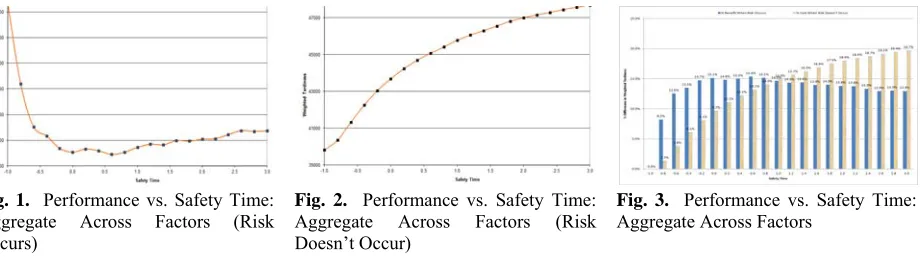
in aggregate. Fig. 1 displays mean weighted tardiness results for Case 1 across the various safety time values. Recall Case 1 corresponds to when ST is used for job prioritization and the job risk actually
530
Fig. 1. Performance vs. Safety Time:
Aggregate Across Factors (Risk Occurs)
Fig. 2. Performance vs. Safety Time:
Aggregate Across Factors (Risk Doesn’t Occur)
Fig. 3. Performance vs. Safety Time:
Aggregate Across Factors
Fig. 2 displays total weighted tardiness results for Case 2. Case 2 corresponds to when ST is used for
job prioritization, but the risk does not materialize. These results are shown primarily for confirmatory purposes since it is intuitive that, if the risk does not occur, then including no safety time should yield the best performance. Indeed, this is true since the best ST value occurs at ‒1.0, which corresponds to
prioritizing jobs using only their nominal processing times.
Fig. 3 displays the percent performance increase (Cases 1 vs. 4) and decrease (Cases 2 vs. 3) when risk does and does not occur, respectively. These results are also aggregated across risk, percent risky jobs and tardiness factor levels. Performance gains exceeds losses within the ST interval, [‒0.8, 0.8], with ST = 0.6 yielding the highest benefit. As expected, the percentage decrease in performance (i.e.,
“cost”) associated with using safety time when the risk does not materialize rises as ST increases.
These results are consistent with Fig. 1 and Fig. 2.
Let us now examine benefit-cost tradeoffs at various ST values, which are important when uncertainty
exists in whether or not the risk will occur. In such cases, the scheduler may ask, “What can I gain in performance vs. what can I lose?” Obviously, the “best” ST value will depend on the likelihood the risk will materialize. Referencing Fig. 3 at ST = ‒0.8, the benefit (13.5%) is 6.3 times greater than the cost (6.1%). For ST = ‒0.4, the benefit (8.2%) is 2.2 times greater than cost (1.3%). At ST = 0, benefit
still exceeds cost by a factor of 1.55. Recall ST = 0 corresponds to prioritizing jobs using the expected
risk times. For example, referencing Eq. 2, if nominal time is 20 minutes and risk level is 0.5, the expected risk time is 20 x 0.5 = 10 minutes (one-half of nominal). If risk level is 2.0, the expected risk time is 20 x 2 = 40 minutes (2 times nominal). If risk level 2.0 and ST = 1.0, the planned risk time is 20
x 2 x 2 = 80 minutes (4 times nominal). Consequently, although ST = 0.6 provides the greatest percent
gain when the risk occurs, ST = 0.6 or ‒0.8 may be “safer” values to use when uncertainty exists in
whether the risk will materialize. These summary results also indicate that, when uncertainty exists, the mean performance gain when the risk occurs will significantly exceed the mean performance loss when it doesn’t occur when using ST within the interval [‒ 0.8, 0] (p = 0.000035).
Thus far, we have only analyzed performance in aggregate. We now examine it at specific factor settings. Fig. 4 shows percent benefit-cost at the low risk level (rj= 0.5). Here, performance gains
exceed losses within a narrower ST interval [‒0.8, 0] than in the aggregate case. Moreover, gains and
losses are lower than the aggregate case. It is interesting to note that performance gain when the risk occurs can become negative at very high ST values (ST≥ 2.4) implying that, under low risk, using too
much safety time can result in worse performance than using none at all.
Fig. 5 shows benefit-cost relationships at the high risk level (rj= 2.0). Performance gains and losses
Fig. 4. Performance vs. Safety Time:
Low Risk Level Fig. 5.High Risk Level Performance vs. Safety Time: Fig. 6.10% Risky Jobs Level Performance vs. Safety Time: Figs. 6-8 display benefit-cost relationships at the three percent risky job levels, 10%, 30% and 50%, respectively. Performance gains and losses are lowest when only 10% of the jobs are risky (on average) and highest when 50% of the jobs are risky, which again is intuitive. However, it is interesting to note the ST interval within which gains exceed losses is much wider for 10% risky jobs
than for 30% or 50%. At 10% risky jobs, gains exceed losses for any ST≤ 2.4. Again, the “best” ST
value to use will depend upon the likelihood the risk will materialize.
Fig. 7. Performance vs. Safety Time:
30% Risky Jobs Level Fig. 8.50% Risky Jobs Level Performance vs. Safety Time: Fig. 9.0.1 Tardiness Factor Level Performance vs. Safety Time: Figs. 9-11 display benefit-cost relationships at the three tardiness factor levels, 0.1, 0.4 and 0.7, respectively. In these cases, performance gains and losses are highest under the lowest TF setting (0.1), which is intuitive since more slack exists in the schedule relative to due dates for the R&M rule to re-sequence jobs. However, the ST interval within which gains exceed losses is much wider at the 0.7
level (70% tardy jobs on average) than at either the 0.1 or 0.4 levels.
Although weighted tardiness performance has been the focus thus far, we conclude this section by examining the rate at which risky jobs are offloaded to the slow machine. Fig. 12 displays the percent risky jobs processed on the slow machine in the scenarios when safety time is/is not utilized in priority assignments (Cases 1 and 4). In aggregate across all factors, 34.2% of risky jobs are offloaded to the slow machine when safety time was not used (and the equivalent case when ST = ‒1). This result is intuitive given the 2:1 speed advantage of the fast machine (i.e., 1/3 of jobs on slow machine and 2/3 jobs on fast machine to balance makespan). When safety time is used, the percent risky jobs assigned to the slow machine increases to 40-45%, depending on safety time.
Fig. 10. Performance vs. Safety Time:
532
Although graphs at specific risk, percent risk job and tardiness factor settings are not shown, the 40-45% rate is fairly consistent across those levels. This rate is reasonable given the proposition used to load the machines (Morton and Pentico, 1993) whereby the highest priority job is assigned to the machine expected to finish it first. Risky jobs are only shifted to the slow machine during times when the schedule is tight (i.e., peak load) and job slack is low.
6. Conclusion and Future Directions
This paper has extended the aversion dynamics research agenda from the single-machine environment to the parallel, proportional two- machine environment to study the effects of empirically observed risk mitigation strategies associated with offloading perceived risky jobs onto a secondary machine. A theoretical proposition (Morton and Pentico, 1993) was used to load the highest priority job on the machine that was expected to finish it first, and the R&M bottleneck dynamics-based heuristic (Morton et al. 1995; Morton and Pentico, 1993) was used to compute job priorities. Four major cases were considered relative to the risk materializing or not and relative to whether or not safety time was applied to processing times within the R&M rule to model risk aversion. Within each major case, two risk levels, three percent risky job levels and three tardiness factor levels were examined across a wide range of potential safety time values. Results indicated that performance gains achieved when risk materializes exceeds performance losses when risk does not materialize within specific safety time intervals. Performance gains and losses were highest at the high risk, high percent risky jobs and/or low tardiness factor settings. Moreover, the ST interval within which gains exceed losses is widest at
the high risk, low percent risky jobs and/or high tardiness factor settings. Lastly, we examined the percentage of risky jobs that were offloaded to the slow machine. Results indicated a substantially higher percentage of risky jobs were assigned to the slow machine when safety time was used, thus validating the intended risk aversion behavior under consideration.
Future directions in aversion dynamics research can take on various forms (McKay and Black, 2006; McKay, et al. 2002). The subject of this paper, the parallel machine environment, can be extended to consider more than the two machines with multiple speed factors. Further, these concepts can be extended to the general job shop or flow shop environments. Moreover, machine risk can be considered as opposed to job risk, thus placing the focus on specific machines as opposed to specific jobs. Furthermore, extensions to the anticipatory batch insertion research agenda can be pursued as detailed in Black, et al. (2008).
Acknowledgements
This paper would not have been possible without the long term encouragement and inspiration of Thomas Morton (Professor Emeritus – Carnegie Mellon University). He helped develop the initial foundations for Aversion Dynamics and provided the guidance and insights necessary to bring the ideas
forward. Dr. Morton also provided valuable guidance as the parallel machine problem was formulated and the research planned.
References
Aytug, H, Lawley, M.A., McKay, K.N., Mohan, S., & Uzsoy, R. (2005). Executing production schedules in the face of uncertainties: a review and some future directions. European Journal of Operations Research, 165, 86-110.
Black, G.W. (2001), Predictive, stochastic and dynamic extensions to aversion dynamics scheduling,
Ph.D. dissertation, University of Alabama in Huntsville.
Black, G.W., McKay, K.N., & Messimer, S.L. (2004). Predictive, stochastic and dynamic extensions to aversion dynamics scheduling. Journal of Scheduling, 7, 277-292.
Black, G.W., McKay, K.N., & Morton, T.E. (2006). Aversion scheduling in the presence of risky jobs.
European Journal of Operational Research, 175(1), 2006, 338-361.
Black, G.W., McKay, K.N., & Varghese, S.E. (2008). ‘Anticipatory batch insertion’ to mitigate perceived processing risk. International Journal of Production Research, 46(4), 853-871.
Cao, Q., Patterson, J.W., & Griffin, T.E. (2001). On the operational definition of processing time uncertainty. International Journal of Production Research, 39(13), 2833-2849.
Cowling, P., & Johansson, M. (2002). Using real time information for effective dynamic scheduling.
European Journal of Operational Research, 139, 230-244.
Dubois, D., Fargier, H., & Fortemps, P. (2003). Fuzzy scheduling: modeling flexible constraints vs. coping with incomplete knowledge. European Journal of Operational Research, 147, 231-252.
Kanet, J.J., & Sridharan, V. (2000). Scheduling with inserted idle time: problem taxonomy and literature review. Operations Research, 48(1), 99-110.
Kleijnen, J.P., & Gaury, E. (2003). Short-term robustness of production management systems: a case study. European Journal of Operational Research, 148(2), 452-465.
McKay, K.N. (1992). Production planning and scheduling: a model for manufacturing decisions
requiring judgment. Ph.D. Thesis, University of Waterloo.
McKay, K.N., Safayeni, F.R., & Buzacott, J.A., (1995). Common sense realities of planning and scheduling in printed circuit board production. International Journal of Production Research, 33(6),
1587-1603.
McKay, K.N., & Wiers, V.C.S. (1999). Unifying the theory and practice of production scheduling.
Journal of Manufacturing Systems, 18(4), 241-255.
McKay, K.N., Morton, T.E., Ramnath, P., Wang, J. (2000). Aversion dynamics – scheduling when the system changes. Journal of Scheduling, 3, 71-88.
McKay, K.N., Pinedo, M., & Webster, S. (2002). A practice-focused agenda for production scheduling research. Production and Operations Management, 11, 249-258.
McKay, K.N., & Black, G.W. (2006). Aversion dynamics – adaptive production control heuristics incorporating risk. Journal of the Operations Research Society of Japan, 49(3), 152-173.
Morton, T.E., & Pentico, D.W. (1993). Heuristic Scheduling Systems, New York: John Wiley & Sons.
Morton, T.E., Narayan, V., Ramnath, P. (1995). A tutorial on bottleneck dynamics: a heuristic scheduling methodology. Production and Operations Management, 4(2), 94-107.
O’Donovan, R, Uzsoy R., & McKay, K.N. (1999). Predictable scheduling and rescheduling on a single
machine in the presence of machine breakdowns and sensitive jobs. International Journal of
Production Research, 37, 4217-4233.
Ovackik, I.M., & Uzsoy, R. (1994). Rolling horizon algorithms for single machine dynamic scheduling problem with sequence dependent setup times. International Journal of Production Research, 32,
1243-1263.
Ovackik, I.M., & Uzsoy, R. (1995). Rolling horizon procedures for dynamic parallel machine scheduling with sequence dependent setup times. International Journal of Production Research, 33,
3173-3192.
Shafaei, R., & Brunn, P. (1999). Workshop scheduling using practical (inaccurate) data Part 1: the performance of heuristic scheduling rules in a dynamic job shop environment using a rolling time horizon approach. International Journal of Production Research, 37(17), 3913-3925.
Shafaei, R., & Brunn, P. (1999). Workshop scheduling using practical (inaccurate) data Part 2: an investigation of the robustness of scheduling rules in a dynamic and stochastic environment.
International Journal of Production Research, 37(18), 4105-4117.
534
Appendix A: Summary of Experimental Results
ST ST ST ST ST ST ST ST ST ST ST ST ST ST ST ST ST ST ST ST
Case Risk % Risky TF -1.0 -0.8 -0.6 -0.4 -0.2 0.0 0.2 0.4 0.6 0.8 1.0 1.2 1.4 1.6 1.8 2.0 2.2 2.4 2.6 2.8
1 0.5 10% 0.1 10701 10487 10362 10348 10453 10294 10445 10387 10611 10524 10586 10862 10934 10973 11061 11180 11219 11261 11413 11488 11 1 0.5 10% 0.4 37917 37369 37143 37000 36310 36263 36325 36513 36576 36793 36978 37163 37287 37277 37235 37321 37339 37552 37547 37562 37 1 0.5 10% 0.7 84994 84646 83452 83738 83265 83441 83510 83676 83643 83733 84107 84312 84477 84575 84636 84706 84832 84827 85058 85053 85 1 0.5 30% 0.1 15820 16205 15623 15701 15443 15597 16075 16165 15945 16475 16869 16813 16790 16745 17012 17063 17246 17317 17081 17144 17 1 0.5 30% 0.4 46205 45030 44314 44002 44462 43902 44436 44458 44856 45307 45849 46051 46267 46536 46507 46887 46830 46781 46794 46888 46 1 0.5 30% 0.7 95713 94429 93763 93166 92322 92418 92559 92721 92899 93323 94162 94427 94560 95040 95211 95090 95481 95765 96207 96489 96 1 0.5 50% 0.1 24282 23623 23043 22650 22518 22490 23117 23661 23239 23978 23796 23521 23366 23843 23968 24231 24091 24550 24938 24695 24 1 0.5 50% 0.4 57720 56588 55313 55050 53749 54427 55151 54947 54881 55604 55839 55696 55638 56496 55871 56161 57006 57370 57796 57957 57 1 0.5 50% 0.7 108569 107172 105485 104786 104875 104559 104796 104461 104371 104979 105357 106214 107267 107476 107790 108429 108220 108896 109069 109051 10 1 2.0 10% 0.1 22494 19440 19317 18867 18472 18298 17666 17573 17269 16893 16972 17044 17133 16949 16755 16939 16937 16156 17513 17251 17 1 2.0 10% 0.4 54306 46147 44346 44359 42282 42146 42036 42632 42791 42900 43013 43187 43365 43358 43087 43070 43061 42992 43169 43169 43 1 2.0 10% 0.7 102512 93380 90025 89648 89105 89156 89232 89086 89271 89232 89208 89240 89173 89212 89229 89229 89229 89222 89222 89222 89 1 2.0 30% 0.1 52757 47418 41646 41542 39153 37836 36979 37782 37461 38787 37556 38397 38466 39208 39400 38368 38197 38654 39656 39092 38 1 2.0 30% 0.4 90358 78596 72252 71965 68166 68795 68528 68760 67588 67338 67597 67718 67525 68128 67476 67567 67868 68083 68428 68501 68 1 2.0 30% 0.7 144732 127762 118173 117007 115354 115396 115487 115573 115482 116001 115886 116241 116155 116466 116255 116232 116553 116772 116785 116720 11 1 2.0 50% 0.1 95223 81654 77539 76359 73388 71810 75137 72950 68972 68275 70721 69697 70058 71182 70855 72090 71477 73540 74261 73229 73 1 2.0 50% 0.4 140851 122317 115619 108194 109517 107960 106574 105943 104559 105725 105558 107464 105792 107521 107235 107490 107540 109058 109207 109715 11 1 2.0 50% 0.7 194955 174421 159445 159832 157882 156585 157737 156020 157737 155376 158026 158463 157446 156631 157300 157627 157147 157306 157568 157500 15
2 0.5 10% 0.1 7742 7732 7768 7829 7873 7918 8016 8057 8178 8342 8430 8517 8737 8926 8950 9120 9180 9272 9418 9493 9
2 0.5 10% 0.4 32676 32702 32741 32872 33050 33242 33475 33751 33934 34231 34470 34666 34905 35132 35237 35515 35618 35817 35926 36004 36 2 0.5 10% 0.7 79036 79031 79286 79530 79872 80231 80718 81115 81423 81678 81979 82345 82646 82831 82952 83203 83335 83492 83618 83667 83 2 0.5 30% 0.1 7742 7782 7788 7935 8087 8269 8473 8681 8981 9110 9299 9447 9671 9951 10129 10315 10555 10655 10894 11061 11 2 0.5 30% 0.4 32676 32709 32904 33287 33674 34185 34679 35145 35600 36146 36747 36926 37368 37812 38238 38677 38889 39088 39382 39607 39 2 0.5 30% 0.7 79036 79222 79681 80392 81124 81989 82912 83742 84460 85224 85985 86706 87272 87736 88086 88439 88869 89164 89574 89773 90 2 0.5 50% 0.1 7742 7751 7859 7992 8089 8292 8464 8584 8817 8969 9201 9408 9503 9745 9961 9995 10257 10322 10623 10752 10 2 0.5 50% 0.4 32676 32765 33062 33371 33790 34430 34918 35326 35883 36502 37050 37475 37730 38221 38819 39212 39512 39838 40145 40564 40 2 0.5 50% 0.7 79036 79265 79830 80660 81754 82683 83830 84788 85696 86555 87430 88261 88834 89463 90225 90679 91188 91645 91966 92381 92 2 2.0 10% 0.1 7742 7873 8178 8737 9180 9635 10033 10274 10606 10702 10724 10839 10858 10938 11001 10913 10961 10966 10915 10881 10 2 2.0 10% 0.4 32676 33050 33934 34905 35618 36085 36499 36705 36985 37050 37295 37520 37515 37657 37792 37790 37854 37788 37967 37967 37 2 2.0 10% 0.7 79036 79872 81423 82646 83335 83761 84057 84174 84265 84313 84393 84455 84476 84500 84510 84510 84510 84536 84536 84536 84 2 2.0 30% 0.1 7742 8087 8981 9671 10555 11195 11794 12334 12755 13015 13294 13584 13791 13881 14113 14229 14172 14177 14334 14315 14 2 2.0 30% 0.4 32676 33674 35600 37368 38889 39888 40672 41454 41895 42291 42829 43158 43315 43497 44019 44182 44304 44403 44549 44568 44 2 2.0 30% 0.7 79036 81124 84460 87272 88869 90003 90585 91038 91238 91470 91617 91739 91798 91865 91909 91916 91924 91992 91990 91993 91 2 2.0 50% 0.1 7742 8089 8817 9503 10257 10904 11421 12029 12373 12841 13128 13508 13624 13810 14204 14446 14533 14620 14777 14884 15 2 2.0 50% 0.4 32676 33790 35883 37730 39512 40720 41848 42939 43441 43931 44687 44882 45695 46093 46509 46788 47220 47272 47325 47645 47 2 2.0 50% 0.7 79036 81754 85696 88834 91188 92770 93743 94306 94680 94972 95251 95483 95557 95736 95814 95824 95830 95912 95922 95967 95
ST ST ST ST ST ST ST ST ST ST ST ST ST ST ST ST ST ST ST ST
Case Risk % Risky TF -1.0 -0.8 -0.6 -0.4 -0.2 0.0 0.2 0.4 0.6 0.8 1.0 1.2 1.4 1.6 1.8 2.0 2.2 2.4 2.6 2.8