OF ULTRASONIC SNOW DEPTH SENSORS
by
Erik Thorsten Boe
A thesis
submitted in partial fulfillment of the requirements for the degree of Master of Science in Hydrologic Sciences
Boise State University
DEFENSE COMMITTEE AND FINAL READING APPROVALS
of the thesis submitted by
Erik Thorsten Boe
Thesis Title: Assessing Local Snow Variability Using a Network of Ultrasonic Snow
Depth Sensors
Date of Final Oral Examination: 04 October 2013
The following individuals read and discussed the thesis submitted by student Erik Thorsten Boe, and they evaluated his presentation and response to questions during the final oral examination. They found that the student passed the final oral examination. James P. McNamara, Ph.D. Chair, Supervisory Committee
Hans-Peter Marshall, Ph.D. Member, Supervisory Committee Alejandro N. Flores, Ph.D. Member, Supervisory Committee
iv
ACKNOWLEDGEMENTS
I would like to thank my advisor, committee, Boise State University staff and students, coworkers, and family for their support during this process. Many thanks to my advisor, Dr. James P. McNamara, for his countless hours of time, encouragement, and well recognized expertise throughout the duration of this investigation. Thanks to my committee, Dr. Hans-Peter Marshall and Dr. Alejandro N. Flores, who were always willing to help and provide a wide breadth of knowledge and advice that was invaluable. Thanks to Pam Aishlin, Patrick Kormos, Dave Eiriksson, Alison Burnop, Brian
Anderson, Alden Shallcross, and others; they were an incredible research group to work with, always willing to lend a hand with technical challenges in the office or spend countless hours in the field. A special thanks to all my amazing kids, sister and brother-in-law, extended family, and friends; they have no idea how much I am thankful for all their support. And finally, I would like to thank my wife Tiara who is the most patient, encouraging, and helpful person I have ever known; I am forever grateful.
v ABSTRACT
During the 2009-2010 winter season, 21 inexpensive ultrasonic snow depth (USD) sensors were constructed and installed, in addition to two standard Judd USD sensors, at Treeline and Lower Deer Point sites located within the snow dominated Dry Creek Experimental Watershed, near Boise, Idaho. Six USD sensors, including a single Judd Communications USD sensor, were installed at the Treeline site along a northeast to southwest transect of the small 0.02 km2 catchment. Seventeen USD sensors, including a single Judd Communications USD sensor, were installed at Lower Deer Point in a
randomized stratified pattern with respect to aspect and vegetation to reflect the nature of the ridge knob site. The purpose of this study was to investigate the local variability of SWE in the form of new fallen snow and assess how well data obtained from standard precipitation gauges represent local conditions. Spatial distributions of new snow depth were converted to estimated new SWE, based off of the relationship between USD measurements of new fallen snow depth and new fallen snow density estimates collected from storm boards placed in a stratified pattern with respect to USD site locations at Treeline and Lower Deer Point. In all, on a storm by storm basis, Lower Deer Point and Treeline precipitation gauges were found to underestimate water accumulation by
vi
vii
TABLE OF CONTENTS
ACKNOWLEDGEMENTS ... iv
ABSTRACT ... v
LIST OF TABLES ... ix
LIST OF FIGURES ... x
CHAPTER 1: INTRODUCTION ... 1
CHAPTER 2: SITE DESCRIPTION ... 5
CHAPTER 3: METHODS ... 9
3.1 Study Design - Snow Depth Measurements ... 9
3.1.1 Theory of Design ... 9
3.1.2 USD Design ... 10
3.1.3 USD Sensor Networks ... 16
3.2 Determining Estimates of New Fallen SWE Accumulation ... 21
CHAPTER 4: RESULTS ... 25
4.1 General Snow Precipitation Event Conditions ... 28
4.2 Local Variability at Lower Deer Point ... 37
4.3 Local Variability at Treeline ... 40
CHAPTER 5: DISCUSSION ... 44
5.1 The Inexpensive USD Sensor ... 44
viii
5.3 Hydrologic Significance and Potential Uses for Inexpensive Ultrasonic Snow
Depth Senor Networks ... 47
5.3.1 Generating Uncertainty Estimates for Operational Hydrologic Models... 48
5.3.2 Generating Improved Uncertainty Estimates of Observationally Derived Precipitation Data at the Watershed Scale ... 48
5.3.3 Incorporating USD Network Precipitation Measurements with Data Assimilation Methodologies ... 49
5.4 Impact of Solar Radiation on New Fallen Snow Metamorphism ... 50
CHAPTER 6: CONCLUSIONS ... 52
CHAPTER 7: REFERENCES ... 54
APPENDIX A ... 57
Manufacturer Specifications for the XL-MaxSonar EZ2 ... 57
APPENDIX B ... 60
Manufacturer Specifications for the GE-MCS Thermistor ... 60
APPENDIX C ... 61
ix
LIST OF TABLES
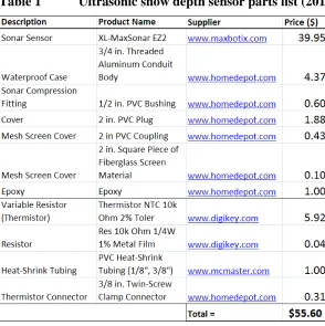
Table 1 Ultrasonic snow depth sensor parts list (2011) ... 14
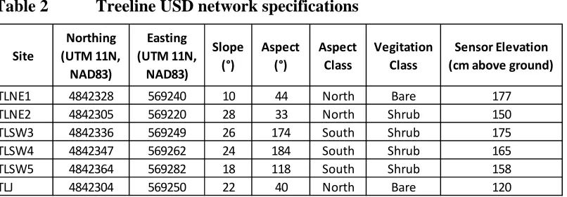
Table 2 Treeline USD network specifications ... 17
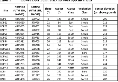
Table 3 Lower Deer Point USD network specifications ... 19
Table 4 Summary table describing variability associated with the lumped bulk new fallen snow density estimate based on sampling new fallen snow densities over the course of 9 precipitation events during the 2011 winter season as described in Section 3.2 ... 24
Table 5 Summary table describing new fallen SWE variability at LDP site ... 40
x
LIST OF FIGURES
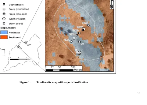
Figure 1 Treeline site map with aspect classification ... 7
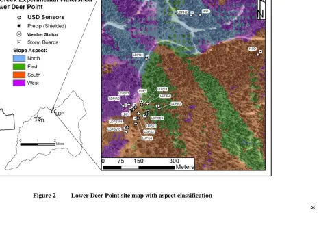
Figure 2 Lower Deer Point site map with aspect classification ... 8
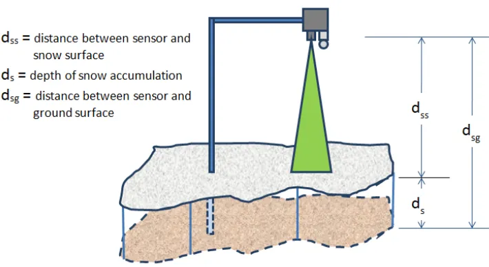
Figure 3 Ultrasonic snow depth sensor illustration ... 10
Figure 4 XL-MaxSonar EZ2 (www.maxbotix.com) ... 12
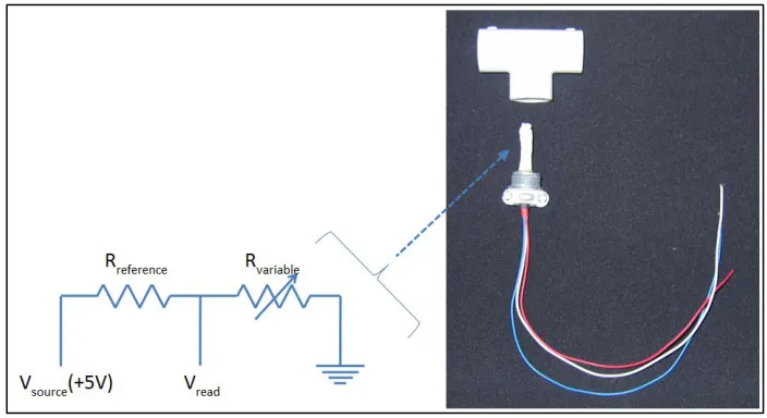
Figure 5 Thermistor design and construction ... 12
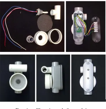
Figure 6 Ultrasonic snow depth sensor design ... 13
Figure 7 Power supply, data acquisition, and installation pictures ... 13
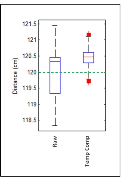
Figure 8 USD sensor performance verification test; box plots describing raw and air temperature compensated distributions of fixed target distance measurements obtained from a randomly selected USD sensor to assess both accuracy, precision, and the degree to which distance measurements are influenced by fluctuations in air temperature. Green line indicates actual target distance while the median, range of values with a 95 percent confidence interval, interquartile range (IQR), and outliers (outside the 95 percent confidence interval) are described by the red line, black whiskers, blue rectangle, and red cross, respectively. ... 15
Figure 9 Picture of ceanothus shrubs compressed below the snow pack at Lower Deer Point; area ceanothus shrubs are typically observed to be approximately 1 meter in height during late spring, summer and fall. ... 18
Figure 10 USD sensors and data acquisition at Lower Deer Point site ... 20
xi
Figure 12 Box plot of lumped bulk new fallen snow density derived from storm board results; the lumped data set includes new fallen snow densities obtained from all storm board locations and storm events; derived from storm board sample results collected during 9 precipitation events
occurring during the 2011 winter season ... 24
Figure 13. Precipitation accumulation during 2010 winter season at LDP ... 27
Figure 14 Wind rose diagram during February 24, 2010 precipitation event at Lower Deer Point (left) and Treeline (right). ... 29
Figure 15 New fallen snow accumulation across representative USD sites at LDP on February 24, 2010; Overlaid with solar radiation, wind speed, air
temperature and calculated effective snow accumulation as measured by the bucket gauge ... 30
Figure 16 New fallen snow accumulation in depth across USD sites at TL on February 24, 2010; Overlaid with solar radiation, wind speed, air
temperature and calculated effective snow accumulation as measured by the bucket gauge (converted to depth using a new snow density of 0.16 g/cm3) ... 31
Figure 17 Wind rose diagram during March 13, 2010 precipitation event at Lower Deer Point (left) and Treeline (right). ... 33
Figure 18 New fallen snow accumulation across representative USD sites at LDP on March 13, 2010; Overlaid with solar radiation, wind speed, air
temperature and calculated effective snow accumulation as measured by the bucket gauge ... 34
Figure 19 New fallen snow accumulation across USD sites at TL on March 13, 2010; Overlaid with solar radiation, wind speed, air temperature, and calculated effective snow accumulation as measured by the bucket gauge ... 35
Figure 20 Wind rose diagram during March 30, 2010 precipitation event at Lower Deer Point (left) and Treeline (right). ... 36
Figure 21 New fallen snow accumulation across representative USD sites at LDP on March 30, 2010; Overlaid with solar radiation, wind speed, air
temperature and calculated effective snow accumulation as measured by the bucket gauge ... 37
xii
(IQR), and outliers (outside the 95 percent confidence interval) are described by the blue diamond, red line, black whiskers, blue rectangle, and red cross, respectively. ... 39
Figure 23 Box plots corresponding to new fallen estimated SWE accumulation, using a constant density, with respect to vegetation class for LDP sites .. 40
Figure 24 Box plots of new fallen SWE with respect precipitation measurements at Treeline. With regards to the box plots, the mean value, median, range of values with a 95 percent confidence interval, interquartile range (IQR), and outliers (outside the 95 percent confidence interval) are described by the blue diamond, red line, black whiskers, blue rectangle, and red cross, respectively. ... 42
CHAPTER 1: INTRODUCTION
Water stored as snow provides approximately 80 percent of streamflow and the vast majority of fresh water for domestic and irrigation purposes in the Western United states (Pagano and Garen, 2005). Add to this the well documented occurrences of increased climate variability and population growth, we find that significantly more pressure is being placed on hydrologic modeling as the basis for decisions regarding water resource policy, management, regulation, and program evaluation (Larson and Peck, 1974; Haan et al., 1995; Kunkel et al., 2007; Harmel and Smith, 2007). A greater understanding of uncertainties associated with streamflow forecasts is essential for operational hydrologic models (Larson and Peck, 1974; Goodison, 1978; Peck, 1997; Yang et al., 2000; Slater and Clark, 2006; Harmel and Smith, 2007).
In snow dominated catchments, streamflow forecast models must account for the spatial and temporal nature of snow water input into the system (Peck, 1997; Clark and Slater, 2006; Slater and Clark, 2006; Elder et al., 2009). This is accomplished by
incorporating snowmelt models, such as SNOW-17 (Anderson, 1973) and the Snowmelt-Runoff Model (Martinec et al., 2008; Burnop, 2012), that route snowmelt water into the system based on local precipitation and temperature observations obtained from
processes (Vicens et al., 1975; Slater and Clark, 2006; Harmel and Smith, 2007). Of these sources of uncertainty, measurement (forcing) uncertainty is commonly regarded as an important factor influencing model performance but is rarely quantified (Larson and Peck, 1974; Peck, 1997; Yang et al., 2000; Slater and Clark, 2006; Harmel and Smith 2007). In particular, precipitation measurements used as model forcings are considered by many as the most important factor to successful hydrologic models (Larson and Peck, 1974; Peck, 1997; Yang et al., 2000). The accuracy of streamflow forecasts in snow dominated catchments is primarily influenced by the accuracy of the snow accumulation and resulting snow water equivalent (SWE) estimates (Slater and Clark, 2006; Elder et al., 2009). Herein lies the challenge, snow precipitation observations are obtained from gauges with high gauge catch deficiencies (Larson and Peck, 1974; Yang et al., 2000; Dingman, 2008), which introduce significant and unknown uncertainties into snowmelt models (Harmel and Smith, 2007).
fence have reduced gauge catch deficiencies and continued tests have improved gauge catch deficiency estimates (Yang et al., 2000; Hansen and Davies, 2002; Fassnacht, 2004; Sevruk et al., 2009) the fact remains that significant errors are present and difficult to ascertain. An important note is that when considering these errors, especially as they relate to local conditions, one cannot overlook the impact of uncertainty associated with natural processes. The variable nature of natural controls such as wind, temperature, slope, aspect, and vegetation-type are contributing factors to precipitation measurement uncertainty as a whole. The act of quantifying measurement uncertainty of local conditions inherently captures uncertainty associated with influential natural processes. All of which begs the question of how representative snow precipitation gauge
measurements are of local conditions. To answer this question, one must look at alternative approaches of snow precipitation measurement. One such method involves the use of ultrasonic snow depth (USD) sensors (Goodison et al., 1984; Goodison et al., 1988; Ryan et al., 2008a,b).
Surface Observation System (ASOS) network in an effort to replace human observers with automated sensors for monitoring snow accumulation. As part of this program, 3 USD sensors were placed at each of 17 NWS monitoring locations over the course of the 2006-2007 winter season. Important conclusions include: (1) incorporating multiple USD sensors improved the overall accuracy of site snow accumulation measurements and (2) even at sites with exposure to significant winds, the network of 3 USD sensors
CHAPTER 2: SITE DESCRIPTION
The study was conducted at Treeline and Lower Deer Point sites situated within the greater Dry Creek Experimental Watershed (DCEW, 27 km2) located to the north of Boise, Idaho.
The Treeline site is located in a vegetation transition zone at the edge of a sagebrush steppe ecotone just below the mixed conifer forested regions of the DCEW (Williams et al., 2009; Anderson, 2011; Eiriksson, 2012). Historically, Treeline receives a mix of rain or snow throughout the winter season with relative weightings varying from year to year. Treeline encompasses 0.02 km2 and is located at an elevation of 1620 m (Williams et al., 2009). The catchment trends from northwest to southeast with steep opposing northeast and southwest slope aspects. Treeline is outfitted with standard meteorological instrumentation that includes two weighing bucket precipitation gauges, one of which is equipped with an Alter shield, and a Judd Communications ultrasonic snow depth sensor (Figure 1). The two precipitation gauges and ultrasonic snow depth sensor are located on the northeast slope. Historically, Treeline is located within a rain-snow transition elevation zone.
7
8
CHAPTER 3: METHODS
3.1 Study Design - Snow Depth Measurements
Ultrasonic snow depth instruments have been widely used to measure snow accumulation in recent years having been under development since the early 1980s (Goodison et al., 1984; Ryan et al., 2008a,b). However, large networks of ultrasonic sensors have not been implemented due to large upfront costs associated with equipment purchases. Obtaining a spatially and statistically significant number snow accumulation observations using ultrasonic sensors that are low cost along with performance
characteristics comparable to commercially available alternatives solicits a novel approach for this investigation. The following inexpensive snow depth sensors were designed, constructed, and tested to meet both the scope and budget of the study.
3.1.1 Theory of Design
Ultrasonic snow depth sensors operate by emitting an ultrasonic pulse (40 kHz to 50 kHz) and measuring the time it takes for the sound pulse to reflect off the surface of the snow and return to the transceiver (Goodison et al., 1984, Ryan et al.; 2008a,b). Since the velocity of sound waves vary as a function air temperature, ultrasonic velocity must be compensated with Equation (1) obtained from Ryan et al. (2008a,b).
The ultrasonic pulse is projected downward in the shape of a cone, as illustrated in Figure 3, with incident angles between approximately 10 and 20 degrees depending on transceiver specifications. The base of the cone (Figure 3) must be clear of all objects (shrubs, hardware, etc) to prevent signal interference.
Figure 3 Ultrasonic snow depth sensor illustration
3.1.2 USD Design
The USD Design for this study was composed of an XL-MaxSonar EZ2
The analog XL-MaxSonar EZ2 device requires three soldered pin connections for operation: (1) supply voltage of 5 volts, (2) connection to ground, and (3) analog output voltage. Over a 0 to 5 volt range, the analog output voltage signal is directly
proportional to the distance between the transceiver and the surface by which the sound wave is reflected. MaxBotix, Inc. specifies a scaling factor of 0.0098 volts per inch
(www.maxbotix.com). Manufacturer specifications for the XL-MaxSonar EZ2 are
included in Appendix A. The thermistor package design involves a variable resister (thermistor) and reference resistor wired into a basic voltage divider circuit (Figure 5). Since air temperature is proportional to the resistance measured across the variable resistor, recorded voltage signals across the variable resistor can be used to determine air temperature. Similar to the transceiver, the thermistor and reference resistor package requires three soldered connections for operation: (1) supply voltage of 2.5 volts, (2) connection to ground, and (3) analog output voltage. Over a 0 to 2.5 volt range, the analog output voltage signal is directly analogous to air temperature using the relationship provided by the manufacturer, GE Measurement and Control Solutions
(www.ge-mcs.com), in Appendix B.
in a small insulated igloo container for protection from environmental conditions next to the base of the fence post (Figure 7).
Figure 4 XL-MaxSonar EZ2 (www.maxbotix.com)
Figure 6 Ultrasonic snow depth sensor design
Table 1 Ultrasonic snow depth sensor parts list (2011)
USD Accuracy and Uncertainty Estimate
“Temp Comp” corresponds to distance measurements compensated for fluctuations in air temperature as described in Section 3.1.2. Results presented in Figure 8 suggest the following: (1) The USD sensors appear to effectively operate within the 1 cm resolution specification of commercially available alternatives such as the Judd Communications model. (2) With the interquartile range (75th percent quartile minus the 25th percent quartile) changing from 1.2 cm to 0.4 cm, air temperature compensation appeared to be both an effective and critical step to produce accurate snow accumulation measurements with higher precision.
Figure 8 USD sensor performance verification test; box plots describing raw
3.1.3 USD Sensor Networks
Treeline USD Sensor Network
Treeline catchment can be described as sagebrush steppe ecotone with a classic symmetrical basin shape composed of opposing northeast and southwest slopes (between 10 and 35 degrees), all of which routes water to an ephemeral stream that leads to a single pour point (Figure 1). Table 2 identifies the location, aspect, slope, and vegetation
Table 2 Treeline USD network specifications
Lower Deer Point USD Sensor Network
Lower Deer Point site is characterized as a ridge knob surrounded locally by shrubs and a mixed conifer forest. Here, consistent with findings by Jost et al. (2007), a randomized stratified pattern with respect to aspect and vegetation class was
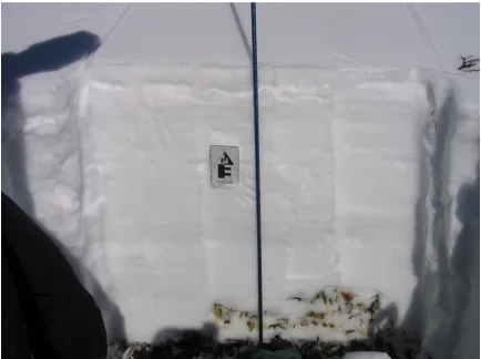
implemented for placement of the USD sensors. In all, 16 USD sensors were installed at Lower Deer Point in a randomized stratified pattern with respect to aspect and vegetation to reflect the nature of the site (Figure 10, Table 3). Each USD sensor was connected to a standalone 7 amp hour power supply and 4-channel U12 HOBO datalogger that collected voltage signals corresponding to snow accumulation and air temperature at 15 minute intervals (Figure 7). At installation sites with heavy ceanothus shrubs present, the USD sensor was placed above and pointed at the top of the shrubs. Previous field observations at Lower Deer Point during spring melt revealed all of the ceanothus shrubs and other bushes to be compressed downslope. This previous knowledge was investigated during the 2010 winter season, at which time a 1 m2 area of the snow pack was excavated to expose the nature of the compressed ceanothus shrubs at a random location (Figure 9). The ceanothus was compressed and pointed downslope, which supports the notion that
Site
Northing
(UTM 11N,
NAD83)
Easting
(UTM 11N,
NAD83) Slope (°) Aspect (°) Aspect Class Vegitation Class
both the weight of the snow pack and forces induced by downslope creep act to compress the shrubs to the base of the snow pack during the winter season.
Figure 9 Picture of ceanothus shrubs compressed below the snow pack at
Table 3 Lower Deer Point USD network specifications
Site
Northing
(UTM 11N,
NAD83)
Easting
(UTM 11N,
NAD83)
Slope
(°)
Aspect
(°)
Aspect
Class
Vegitation
Class
3.2 Determining Estimates of New Fallen SWE Accumulation
At any given site, SWE is equivalent to the product of the local bulk density and depth of snow (Jonas and Magnusson, 2009; Sturm et al., 2010). For this study, new fallen SWE associated with each precipitation event was estimated by Equation (3), where
ns and hns are the density and accumulation of new fallen snow, respectively.(3)
To quantify the densities of new fallen snow at Treeline and Lower Deer Point, storm boards were placed at Treeline (Figure 1) and Lower Deer Point (Figure 2) to collect new fallen snow. Fourteen white HDPE storm boards were placed in a spatially stratified pattern with respect to site, aspect, and vegetation as illustrated in Figure 1 and Figure 2. New fallen snow density estimates for 9 precipitation events for each site were recorded. Within 6 hours after a snow precipitation event
concluded, new fallen snow densities on the storm boards were determined using a Snowmetrics 12 inch SWE tube and scale (www.snowmetrics.com) as follows with the assumption that the basal layer was effectively incompressible and any down-slope movement of the snowpack was insignificant over the period of precipitation accumulation.
1. Insert tube into new fallen snow with vertical motion; where dtube is
the inside diameter of the SWE tube.
2. Record snow depth to nearest 2 mm increment (hns).
3. Hang SWE tube from scale hook to determine weight (wns).
4. Calculate new fallen snow density using Equation (2)
(www.snowmetrics.com); where ns is new fallen snow density.
New fallen snow densities obtained from all storm board locations are presented in Figure 11 and Figure 12. Box plots were selected to describe the variability because they allow both a qualitative and quantitative assessment of variability. With regards to the box plots presented in this report, the mean, median, range of values with a 95 percent confidence interval, interquartile range (IQR), and outliers (outside the 95 percent
Figure 12 Box plot of lumped bulk new fallen snow density derived from storm board results; the lumped data set includes new fallen snow densities obtained from all storm board locations and storm events; derived from storm board sample results collected during 9 precipitation events occurring during the 2011 winter season
Table 4 Summary table describing variability associated with the lumped bulk
CHAPTER 4: RESULTS
Snow precipitation events occurring on February 24, 2010, March 13, 2010, and March 30, 2010 were included as case studies for this investigation because all USD sensor sites (1) received snow accumulation on dense basal layer, (2) all USD sensor sites were operable with the exception of LDPE3, which appeared to have a faulty transceiver, and (3) air temperatures were below freezing prior to onset and during snowfall (Figure 13). Including only sites that experienced precipitation events while air temperatures were below 0 °C allowed for the assumption that the basal layer was effectively
27
Figure 13. Precipitation accumulation during 2010 winter season at LDP ‐15 ‐10 ‐5 0 5 10 15 20 25 30 0 50 100 150 200 250 300 350 400 450 500 550 12/30/ 09 01/13/ 10 01/27/ 10 02/10/ 10 02/24/ 10 03/10/ 10 03/24/ 10 04/07/ 10 04/21/ 10 05/05/ 10 05/19/ 10 06/02/ 10 06/16/ 10 06/30/ 10 Air Te m p e ra tu re (° C) Pr e ci p it at io n A ccu m u la ti o n (m m ) Date Precip (mm) Air Temp (°C)
4.1 General Snow Precipitation Event Conditions
During the February 24, 2010 precipitation event, air temperature was below 0°C and wind speeds of 5 to +15 m/s were observed from the southeast at both Lower Deer Point and Treeline sites (Figure 14, Figure 15, and Figure 16). The dense and effectively incompressible basal layer assumption was supported by little previous snowpack
densification before the storm, as the last precipitation event occurred 12 days earlier on February 12, 2010. Air temperature reached as high as 3.5°C with clear skies allowing full exposure to incoming solar radiation (Figure 15 and Figure 16) during the period of snowpack densification that occurred prior to the cold front and subsequent snow precipitation event on February 24, 2010. At Lower Deer Point, new fallen snow
accumulation appeared consistent with bucket gauge observations (Figure 15). The range of new fallen snow accumulation was approximately 5 cm, centered about the bucket gauge observations. Sites located at wind shielded vegetation zones (LDPN1, LDPSE1, LDPS1) recorded larger snow depth changes snow than windward sites (LDPSW4, LDPW1), which all in turn recorded greater depth changes than the forested canopy sites (LDPN2). At Treeline, representative new fallen snow accumulation appeared more variable with respect to bucket gauge observations, likely influenced by the wind out of the southeast (Figure 14 and Figure 16) during snow precipitation. Ridge sites (TLNE1, TLSW5), with similar wind exposures, experienced similar accumulation of new fallen snow. Mid-slope sites with opposing northeast and southwest aspects (TLJ, TLSW4) appeared to experience moderate differential accumulation along with significant differences in densification and redistribution upon storm cessation (Figure 16).
15 feet up-gradient from the ephemeral channel, experienced similar new fallen snow accumulation. The range of new fallen snow accumulation was approximately 9 cm of snow depth.
Figure 14 Wind rose diagram during February 24, 2010 precipitation event at
Figure 16 New fallen snow accumulation in depth across USD sites at TL on February 24, 2010; Overlaid with solar radiation, wind speed, air temperature and calculated effective snow accumulation as measured by the bucket gauge (converted
to depth using a new snow density of 0.16 g/cm3)
During the March 13, 2010 precipitation event, air temperature was below 0°C and wind speeds of 5 to +15 m/s were observed from the northwest from both Lower Deer Point and Treeline sites (Figure 17, Figure 18, and Figure 19). The dense and effectively incompressible basal layer assumption was supported by previous snowpack
metamorphism occurring since the last significant precipitation event on February 24, 2010 between which time there was light accumulation of snow on March 9, 2010. Air temperature reached as high as 7 °C with partially clear skies allowing for moderate exposure to incoming solar radiation (Figure 16) during the period of snowpack metamorphism that occurred prior to the cold front and subsequent snow precipitation event on March 13, 2010. At Lower Deer Point, representative new fallen snow accumulation appeared consistent with bucket gauge observations (Figure 18). All representative sites with the exception of LDPN1 and LDPW1 accumulated less snow depth than estimated from the bucket gauge, using a constant density of 0.16 g/cm3.
Aspect and vegetation class controls on snow depth did not appear present. At Treeline, representative new fallen snow depth was highly variable, likely influenced by variability associated with wind speed and direction (Figure 17, Figure 18, and Figure 19), as well as variability in new snow density and densification rates. Aspect class controls did not appear present.
Twenty-four hours after storm cessation, all sites at Lower Deer Point and Treeline with a southern exposure experienced significant decline in apparent depth compared to sites with northern exposures. This decrease in depth appears to correlate strongly with exposure to solar radiation (Figure 18 and Figure 19), which leads to two potential explanations. Since snow temperature is one of the primary drivers of
the snowpack due to creep, a phenomenon that was inadvertently observed by the movement of caution flags marking USD sensor sites on occasion.
Figure 17 Wind rose diagram during March 13, 2010 precipitation event at
Figure 18 New fallen snow accumulation across representative USD sites at LDP on March 13, 2010; Overlaid with solar radiation, wind speed, air temperature and calculated effective snow accumulation as measured by the bucket gauge
Figure 19 New fallen snow accumulation across USD sites at TL on March 13, 2010; Overlaid with solar radiation, wind speed, air temperature, and calculated effective snow accumulation as measured by the bucket gauge
During the March 30, 2010 precipitation event, air temperature was below 0°C and wind speeds of 5 to +15 m/s (Figure 20 and Figure 21) were observed from the west from both Lower Deer Point and Treeline sites. The dense and effectively incompressible basal layer assumption was supported by little previous snowpack metamorphism prior to the storm, due to the last significant precipitation event 5 days before on March 25, 2010.
Air temperature reached as high as 8 °C during the period of snowpack densification that occurred prior to the cold front and subsequent snow precipitation event on March 30, 2010. As illustrated in Figure 19, representative new fallen snow accumulation was highly variable, likely influenced by the higher sustained wind speeds that originated out of the west (Figure 20 and Figure 21). During the latter 2 hours of the snow
accumulation period, average hourly wind speeds were 19.5 and 16.5 m/s, respectively. Sites located at wind shielded vegetation zones (LDPN1, LDPSE1, LDPS1) accumulated significantly more snow depth than LDPSW4 (exposed to wind) and LDPN1 (forested canopy). Additionally, the variable nature of snow accumulation is highlighted by observed differences between LDPW1 and LDPSW4 wind exposed sites, with snow accumulations of 24.0 cm and 14.5 cm depth respectively. As observed during the March 13, 2010 event, 18 hours after storm cessation a significant decline in accumulated snow depth appears to correlate strongly with exposure to incoming solar radiation (Figure 19).
Figure 20 Wind rose diagram during March 30, 2010 precipitation event at
Figure 21 New fallen snow accumulation across representative USD sites at LDP on March 30, 2010; Overlaid with solar radiation, wind speed, air temperature and calculated effective snow accumulation as measured by the bucket gauge
4.2 Local Variability at Lower Deer Point
USD sensor installation locations at Lower Deer Point followed a randomized stratified pattern with respect to aspect and vegetation class (Figure 2). Box plots describing lumped new fallen SWE variability with respect to precipitation gauge measurements at Lower Deer Point are presented in Figure 22 and Table 5. Here snow
depth change is converted to new SWE using a density of 0.16 g/cm3, in contrast to previous figures that were given in terms of snow depth. Review of accumulation distributions supported the notion that vegetation type was by far the most significant controlling mechanism for new fallen SWE distributions discussed by Jost et al. (2007). As a result, new fallen SWE accumulation data was partitioned into three classifications:
Bare: sites characterized by compressed shrubs (below the snowpack) and significant exposure.
Vegetation transition: sites characterized by compressed shrubs (below the snowpack) and bordering heavy distributions of large exposed shrubs and mixed conifer forested areas.
Canopy: sites located within the mixed conifer forest and below a dense canopy.
our bulk new fallen snow density estimate (Table 4). Assuming one standard deviation as a reasonable estimate of uncertainty, uncertainty associated with bulk new fallen snow density (Table 4), along with uncertainty associated with our new fallen snow
accumulation can be propagated through Equation 3 using Equation 4 (Holman, 2001; Potter et al., 2010) to determine uncertainty associated with calculated SWE estimates presented in Table 5.
∆ ∗ ∆ ∆ (4)
Figure 22 Box plots of new fallen SWE with respect precipitation measurements
Table 5 Summary table describing new fallen SWE variability at LDP site
Figure 23 Box plots corresponding to new fallen estimated SWE accumulation,
using a constant density, with respect to vegetation class for LDP sites
4.3 Local Variability at Treeline
USD sensor installation locations at the Treeline followed a northeast to
Due to the homogeneous nature of the vegetation class, composed nearly entirely of sagebrush and other small shrubs, aspect appeared to be the primary mechanism
controlling accumulation of new fallen SWE. As a result, new fallen SWE accumulation data was partitioned into two classifications:
North: sites characterized by sagebrush and other small shrubs with northeast exposures.
South: sites characterized by sagebrush and other small shrubs with southwest exposures.
accumulation can be propagated through Equation 3 using Equation 4 (Holman, 2001) to determine uncertainty associated with calculated SWE estimates presented in Table 6.
Figure 24 Box plots of new fallen SWE with respect precipitation measurements
at Treeline. With regards to the box plots, the mean value, median, range of values with a 95 percent confidence interval, interquartile range (IQR), and outliers (outside the 95 percent confidence interval) are described by the blue diamond, red line, black whiskers, blue rectangle, and red cross, respectively.
CHAPTER 5: DISCUSSION
5.1 The Inexpensive USD Sensor
Overall, the inexpensive USD sensors developed and constructed for this study performed quite well, all things considered. The USD sensors provided performance characteristics that were consistent with those advertised for commercially available alternatives, attaining an accuracy (bias) within 0.5 cm and a precision of less than 0.32 cm (defining precision as one standard deviation) when tested above a flat concrete slab over the temperature range of 0 to 10 °C. Any future work using these USD sensors should consider the following:
1. During site installation, the USD sensor and internal XL-MaxSonar EZ-2 transceiver needs to be positioned normal to the surface of the snow. The transceiver is very sensitive to interference from either the ground or internal cover, so it is critical that it is tested in the field prior to leaving the site. Physically adjusting the sound pulse direction of the USD sensor or internal transceiver was required at most sites to obtain a true depth signal.
2. Additionally, selection of each USD installation site poses many
that might interfere with the signal from the USD. So when installing USD sensors at a densely vegetated area such as Lower Deer Point, one can either remove all vegetation, rocks, and sticks from the measurement target and rake it flat or simply point the USD sensor at the top of the vegetation. For this study, we selected the latter method. Removing vegetation is no trivial task, and while it does allow for continuous measurement of snow accumulation through the entire winter season, the act appeared to effectively create a vegetation transition site that would catch redistributed snow. Since we were interested in new fallen snow accumulation, not season total, merely pointing the USD sensor towards the ground and at the vegetation sufficed. We found that as soon as the snowpack forms, smaller shrubs such as ceanothus that are less than approximately 1 meter in height were compressed below the snowpack and pointed downslope as described in Section 3.1.3.
3. The USD sensors collect raw, so-called zero order data that is quite noisy. There is no optimized internal algorithm as seen in commercially available alternatives that clean the data. As a result, manual and
qualitative techniques were required to remove outliers associated with our dataset that was collected at 15 minute intervals. It is highly
5.2 Local Variability with Respect to Site Precipitation Gauge Observations
The purpose of this study was to assess local variability of water accumulation in the form of new fallen snow with respect to site precipitation gauge observations using a network of inexpensive USD sensors. Comparing observed variability between Treeline and Lower Deer Point over the course of each storm (Figure 22 and Figure 24, Table 5 and Table 6) found that (1) measures of variability such as range and standard deviation for both locations were more or less the same and (2) variability increases at both locations with increasing snow accumulation. These findings are consistent with what Ryan et al. (2008b) noticed at the 17 NWS-ASOS sites, which were outfitted with 3 USD sensors at each site.
Controls on snow accumulation at a small catchment in a sagebrush steppe ecotone (Treeline) are quite different than that at a ridge knob with a mixed shrubs and conifers (Lower Deer Point). At Lower Deer Point, while differences in the magnitude of snow accumulation can be observed between each precipitation event, a clear trend based on vegetation class appears present (Figure 23). (1) Vegetation transition sites, those with mixed shrubs and bordering conifer forests, experienced the highest snow
accumulation with the lowest variability. (2) Bare sites, with shrubs compressed at the base of the pack, experienced moderate snow accumulation with the highest variability. (3) Canopy sites generally experienced the lowest snow accumulation with moderate variability. With respect to precipitation events occurring on February 24, March 13, and March 30 at Lower Deer Point, weighing-type precipitation gauge underestimates
significant uncertainty themselves. Uncertainty estimates of SWE at Lower Deer Point (Table 5) suggest that the calculated gauge-catch deficiencies have percent uncertainties of ±19%. At Treeline, while differences in the magnitude of snow accumulation can be observed between each precipitation event, no clear trend based on aspect appears present (Figure 25). Likely depending on wind speed and direction, accumulation was more or less consistent on north and south aspects. With respect to precipitation events occurring on February 24, March 13, and March 30 at Treeline, weighing-type precipitation gauge underestimates (gauge-catch deficiencies) were approximately 26%, 26%, and 18%, respectively. However, as described for Lower Deer Point above, it is important to note that these percent gauge-catch deficiencies contain significant uncertainty themselves. Uncertainty estimates of SWE at Treeline (Table 6) suggest that the calculated gauge-catch deficiencies have percent uncertainties of ±19%.
5.3 Hydrologic Significance and Potential Uses for Inexpensive Ultrasonic Snow
Depth Senor Networks
5.3.1 Generating Uncertainty Estimates for Operational Hydrologic Models
The National Weather Service (NWS) stresses the importance and challenges researchers to develop methods by which error estimates can be added to streamflow predictions generated by operational hydrologic models (personal communication, Dr. Pedro Restrepo of the NWS Office of Hydrologic Development Hydrology Laboratory). Findings from this study suggest that, in snow dominated catchments, setting up a
network of USD sensors around meteorological stations can provide value added information with regards to error estimates. More specifically, using the methods outlined above, water accumulation estimates obtained from USD networks placed around meteorological sites enable direct determination of uncertainty estimates
associated with standard precipitation observations such as those obtained from weighing bucket gauges. Subsequent uncertainty estimates, similar to those presented in this study, can then be propagated through the hydrologic model, enabling placement of error bars on output estimates.
5.3.2 Generating Improved Uncertainty Estimates of Observationally Derived Precipitation Data at the Watershed Scale
USD sensor network clusters at these locations would enable field based variability estimates that are more reflective of the watershed.
5.3.3 Incorporating USD Network Precipitation Measurements with Data Assimilation Methodologies
Use of data assimilation methods to improve streamflow forecast model
simulation estimates has been increasing (Houser et al., 1998; Reichle et al., 2002; Slater and Clark, 2006; Clark et al., 2006). Common adaptive methods of data assimilation such as the Kalmen Filter (EKF) or Ensemble Kalmen Filter (EnKF) have the potential to benefit greatly from observational snow precipitation data sets obtained from USD sensor networks.
generated based on estimates of variance, which much like in EKFs, could benefit from using observationally derived data sets to describe the ensemble distributions.
5.4 Impact of Solar Radiation on New Fallen Snow Metamorphism
Metamorphism or densification of a new fallen snow layer is driven by energy exchanges occurring at the interface between the snowpack and the atmosphere (Armstrong and Brun, 2008). The governing energy balance is driven by shortwave (solar) radiation, longwave radiation, sensible heat, latent heat, and to a lesser extent from energy fluxes associated with mass transfer from blowing snow and conduction from the basal layer (Armstrong and Brun, 2008). Above all sources of energy, solar radiation appeared to have significant influence on the rate of densification at both Lower Deer Point and Treeline sites. This was evident by a shift down in the normalized depth of the new fallen snow layer at sites characterized by a southern exposure (Figure 18 and Figure 19). Upon cessation of the March 13, 2010 precipitation event, densification of the new fallen snow layer appeared comparable across all USD sensors at Lower Deer Point and Treeline sites until reaching what could be effectively described as a cliff (shift down) in the apparent depth of the new fallen snow layer. Weather conditions leading to the observed shift at USD sites with southern aspects could be described as having cool temperatures, clear skies, and low wind. At Lower Deer Point, air temperatures were less than 2°C, wind speeds less than 4 m/s and solar radiation reached approximately 800 W/m2 over the course of a smooth diurnal cycle, which indicates clear and sunny
were present throughout the day. The low wind and cool air temperatures would suggest that the impact of sensible and latent heat exchanges were minimal, while the lack of cloud cover eliminates any significant influx of longwave radiation. All of which leads to the conclusion that incoming solar radiation causing increased snow temperature is likely the cause of the accelerated rate of densification of the new fallen snow layer.
The alternate hypothesis that the shift down in apparent new fallen snow depth is a result of lateral downslope movement of the snowpack due to creep is unlikely for a few reasons. (1) While creep was documented in the field by observed movements in caution flags around USD sensor sites along with compressed ceanothus shrubs pointed downslope, significant movements of the snowpack were only observed during warmer spring time conditions at exposed sites characterized with steep slopes. (2) LDPSE1 was one of the USD sites with a southern aspect that experienced a shift down in snow depth. LDPSE1 has a relatively low slope and is located at a vegetation transition site that boarders a heavy distribution of large exposed shrubs and a mixed conifer forested area located downslope and to the north. These conditions would tend to inhibit the
CHAPTER 6: CONCLUSIONS
The purpose of this study was to investigate local variability of SWE in the form of new fallen snow and develop uncertainty estimates to assess how well data obtained from standard precipitation gauges represents local conditions using a network of ultrasonic snow depth sensors. USD sensor networks at Lower Deer Point and Treeline research sites were used to collect snow accumulation time series’ over the course of the 2009-2010 winter season. During this period, three specific snow precipitation events occurring on February 24, 2010, March 13, 2010, and March 30, 2010 were included as case studies in this investigation. The findings of the investigation are as follows.
At Treeline, spatial topographic controls on new fallen SWE accumulation are inconclusive. Accumulation at Treeline site was more or less consistent on both north and south aspects and appeared to be controlled by wind speed and direction. While controls on accumulation could not be explicitly identified, the variability observed during each precipitation event was consistent (Figure 25). With respect to precipitation events occurring on February 24, March 13, and March 30 at Treeline, weighing-type precipitation gauge underestimates (gauge-catch deficiencies) were approximately 26%, 26%, and 18%, respectively. However, as described for Lower Deer Point above, it is important to note that these percent gauge-catch deficiencies contain significant
CHAPTER 7: REFERENCES
Anderson BT. 2011. Spatial Distribution and Evolution of a Seasonal Snowpack in Complex Terrain: An Evaluation of the SNODAS Modeling Product. In: Department of Geosciences, Boise State University.
Anderson EA. 1973. National Weather Service River Forecast System - Snow Accumulation and Ablation Model. Service NW (ed.).
Armstrong RL, Brun E, 2008. Snow and Climate. Cambridge University Press. Burnop AC. 2012. Assessing the Value of Improved Snow Information in Operational
Hydrologic Models. In: Department of Geosciences, Boise State University. Clark MP, Slater AG. 2006. Probabilistic quantitative precipitation estimation in complex
terrain. Journal of Hydrometeorology, 7: 3-22.
Clark MP, Slater AG, Barrett AP, Hay LE, McCabe GJ, Rajagopalan B, Leavesley GH. 2006. Assimilation of snow covered area information into hydrologic and land-surface models. Advances in Water Resources, 29: 1209-1221.
Dingman SL. 2008. Physical Hydrology. 2nd Edn., Waveland Press, Inc.
Eiriksson D. 2012. The Hydrologic Significance of Lateral Water Flow in Snow. In: Department of Geosciences, Boise State University.
Fassnacht SR. 2004. Estimating Alter-shielded gauge snowfall undercatch, snowpack sublimation, and blowing snow transport at six sites in the coterminous USA. Hydrological Processes, 18: 3481-3492.
Goodison BE. 1978. Accuracy of Canadian Snow Gauge Measurements. Journal of Applied Meteorology, 17: 1542-1548.
Goodison BE, Metcalfe J, Wilson B, Jones K. 1988. The Canadian Automatic Snow Depth Sensor: A Performance Update. In: 56th Annual Western Snow Conference.
Haan CT, Allred B, Storm DE, Sabbagh GJ, Prabhu S. 1995. Statistical Procedure for Evaluating Hydrologic Water-Quality Models. Transactions of the Asae, 38: 725-733.
Hansen S, Davies MA. 2002. Windshields for Precipitation Gauges and Improved Measurement Technique for Snowfall. Agriculture USDo (ed.), pp: 1-6.
Harmel RD, Smith PK. 2007. Consideration of measurement uncertainty in the evaluation of goodness-of-fit in hydrologic and water quality modeling. Journal of
Hydrology, 337: 326-336.
Holman JP. 2001. Experimental Methods for Engineers. 7th Edn., McGraw-Hill.
Jonas T, Marty C, Magnusson J. 2009. Estimating the snow water equivalent from snow depth measurements in the Swiss Alps. Journal of Hydrology, 378: 161-167. Jost G, Weiler M, Gluns DR, Alila Y. 2007. The influence of forest and topography on
snow accumulation and melt at the watershed-scale. Journal of Hydrology, 347: 101-115.
Kunkel KE, Palecki MA, Hubbard KG, Robinson DA, Redmond KT, Easterling DR. 2007. Trend identification in twentieth-century US snowfall: The challenges. Journal of Atmospheric and Oceanic Technology, 24: 64-73.
Larson LW, Peck EL. 1974. ACCURACY OF PRECIPITATION MEASUREMENTS FOR HYDROLOGIC MODELING. Water Resources Research, 10: 857-863. Martinec J, Rango A, Roberts R. 2008. Snowmelt Runoff Model (SRM) User's Manual. Pagano T, Garen D. 2005. A recent increase in western US streamflow variability and
persistence. Journal of Hydrometeorology, 6: 173-179.
Peck EL. 1997. Quality of hydrometeorological, data in cold regions. Journal of the American Water Resources Association, 33: 125-134.
Potter K, Kniss J, Riesenfeld R, Johnson CR. 2010. Visualizing Summary Statistics and Uncertainty. Computer Graphics Forum, 29: 823-832.
Reichle RH, Walker JP, Koster RD, Houser PR. 2002. Extended versus ensemble
Kalman filtering for land data assimilation. Journal of Hydrometeorology, 3: 728-740.
Ryan WA, Doesken NJ, Fassnacht SR. 2008. Evaluation of ultrasonic snow depth sensors for U.S. snow measurements. Journal of Atmospheric and Oceanic Technology,
Ryan WA, Doesken NJ, Fassnacht SR. 2008. Preliminary results of ultrasonic snow depth sensor testing for National Weather Service (NWS) snow measurements in the US. Hydrological Processes, 22: 2748-2757.
Sevruk B, Ondras M, Chvila B. 2009. The WMO precipitation measurement intercomparisons. Atmospheric Research, 92: 376-380.
Shallcross AT, McNamara JP, Flores AN, Marshall H, Marks DG, Glenn NF. 2010. Estimating Basin Snow Volume Using Aerial LiDAR and Binary Regression Trees. In: American Geophysical Union.
Slater AG, Clark MP. 2006. Snow data assimilation via an ensemble Kalman filter. Journal of Hydrometeorology, 7: 478-493.
Sturm M, Taras B, Liston GE, Derksen C, Jonas T, Lea J. 2010. Estimating Snow Water Equivalent Using Snow Depth Data and Climate Classes. Journal of
Hydrometeorology, 11: 1380-1394.
Vicens GJ, Rodriguez-Iturbe I, Schaake JC. 1975. BAYESIAN FRAMEWORK FOR USE OF REGIONAL INFORMATION IN HYDROLOGY. Water Resources Research, 11: 405-414.
Williams CJ, McNamara JP, Chandler DG. 2009. Controls on the temporal and spatial variability of soil moisture in a mountainous landscape: the signature of snow and complex terrain. Hydrology and Earth System Sciences, 13: 1325-1336.
APPENDIX A
APPENDIX B
APPENDIX C
Example of Campbell Scientific Edlog Data Acquisition Program Used for the