Volume 36 - Article 48 | Pages 1453–1490

(1)

VOLUME 36, ARTICLE 48, PAGES 1453

,

1490

PUBLISHED 4 MAY 2017

http://www.demographic-research.org/Volumes/Vol36/48/ DOI: 10.4054/DemRes.2017.36.48

Research Article

The welfare state and demographic dividends

Gemma Abío

Concepció Patxot

Miguel Sánchez-Romero

Guadalupe Souto

This open-access work is published under the terms of the Creative Commons Attribution NonCommercial License 2.0 Germany, which permits use, reproduction & distribution in any medium for non-commercial purposes, provided the original author(s) and source are given credit.

(2)

1 Introduction 1454

2 Measuring the demographic dividend: Concepts and methods 1456

3 NTA dataset and welfare state models 1460

4 Results: Decomposing the demographic dividend 1467

4.1 Data and methodology 1467

4.2 Decomposing the demographic dividend 1472 4.3 Understanding the role of welfare state transfers 1476

5 Discussion and conclusions 1481

6 Acknowledgements 1482

References 1482

(3)

The welfare state and demographic dividends

Gemma Abío1 Concepció Patxot2 Miguel Sánchez-Romero3

Guadalupe Souto4

Abstract

BACKGROUND

The demographic transition experienced by developed countries produces initial positive effects on economic growth ‒ the first demographic dividend ‒ which can be extended into a second demographic dividend if baby boomers’ savings increase capital accumulation. Nevertheless, aging might reverse this process if dissaving of elderly baby boomers and the pressure on the pay-as-you-go financed welfare state reduce savings and capital.

OBJECTIVE

The aim of this paper is to evaluate the extent to which demographic dividends in Spain provide an opportunity for the reform of the welfare state system for an aging population.

METHODS

We decompose demographic dividends using a general equilibrium overlapping generations model with realistic demography and public transfers from the National Transfer Accounts database. This allows us to capture the endogenous evolution of savings and capital accumulation and, hence, the second demographic dividend.

RESULTS

When baby boomers enter the labor market, the purely demographic support ratio increases and this positive effect is extended by composition changes in the age structure of workers. When they start saving, the second demographic dividend arises,

1_{Universitat de Barcelona, Spain.}

(4)

while its total net effect depends both on the strength of the aging process and on transfer size.

CONCLUSIONS

The derived decomposition shows that the second demographic dividend might also disappear. Sharp population aging in Spain implies that capital will shrink drastically after 2040. Before this, there seems to be margin for reforms; however, an extension of the welfare state toward the Nordic model would considerably reduce capital.

CONTRIBUTIONS

This paper contributes to the debate on the effects of demographics on economic growth by decomposing demographic dividends and investigating the impact of different welfare state transfer systems on the second demographic dividend.

1. Introduction

The process of economic development experienced by most countries throughout the last century has been accompanied by a demographic transition. On one hand, life expectancy has increased steadily. On the other hand, there has been a decline in fertility, especially after the post-war baby boom. As a result, the population age structure is experiencing a dramatic change, thus impacting economic conditions. The extent to which demographic change affects economic growth ‒ and generates a demographic dividend ‒ has been the subject of investigation in recent decades.5

Relevant literature focuses on a better understanding of the interplay between demographics, economics, and intergenerational transfers. As Williamson (2013) states, the demographic dividend comprises two different effects of the demographic transition on economic growth: the labor participation rate effect and the growth effect. Mason and Lee (2006) distinguish between a first and a second dividend. The first demographic dividend arises when baby boomers enter the labor market: As the working-age population rises, this leads to an increase in economic growth. The second demographic dividend concerns a potential increase in baby boomers’ savings: At a later stage of the aging process, the ratio of capital per worker in the economy increases, enhancing economic growth.

It is worth noting that the first demographic dividend is an automatic and transitional effect. It appears when baby boom cohorts enter the labor market and disappears when they retire. However, the size and length of the second demographic dividend are not so straightforward. Interestingly, the process is not only affected by the

(5)

speed of change in population age structure (Lee, Mason, and Miller 2001) but also by the size and age structure of the national public transfer system. For example, public retirement pensions and private savings are substitutes for income which provide for consumption in old age. Hence, the effects of population aging on savings and capital accumulation depend on the amount of public transfers to the elderly. Moreover, demographic change alters the ratio of beneficiaries to tax payers, putting pressure on public budgets, which are mostly financed on a pay-as-you-go (PAYG) basis.

The lack of longitudinal micro- and macrodata creates complexity when performing empirical research on demographic dividends. Constructing an adequate dataset to analyze the intergenerational economy is the purpose of the National Transfer Accounts Project (NTA), which has developed a methodology, currently applied to more than 40 countries, aimed at measuring how resources are redistributed across age groups through private transfers, public transfers, and asset markets.6_{The NTA}

estimates provide age profiles for all transfer items, consistent to the National Accounts (NA) aggregates. Hence, they reflect both the size and age pattern of welfare state transfers, together with the corresponding private reallocations occurring in each economy.

This paper provides a better understanding of the impact of demographic transition on economic growth by measuring demographic dividends and, simultaneously, investigating the role of public transfer systems on the second dividend. To this end, we implement a general equilibrium overlapping generations model (OLG) with realistic demography, following Bommier and Lee (2003) and Sánchez-Romero et al. (2013). This model explicitly considers savings and capital accumulation as endogenous, which is crucial to capturing the second demographic dividend and how it interacts with the welfare state crisis during the baby boomers’ retirement. We also introduce realistic public transfers from the NTA dataset. We focus on the Spanish case, given the strong demographic transition this country is experiencing. To evaluate the impact of the welfare state configuration, we also select two other countries representative of different welfare state models, Sweden and the United States.

The rest of the paper is organized as follows. Section 2 includes the different concepts and methods developed to measure the demographic dividend to contextualize our approach. Section 3 describes the content of the National Transfer Accounts dataset, and the use of these estimates for analyzing the structure of welfare state transfers. Section 4 presents the analysis, starting with a brief description of the model and data used. Subsequently, the estimates of demographic dividends are presented. Particularly, we opt for decomposing the demographic dividend into three factors: demographic, labor market, and savings. The first two correspond to the first

6_{See www.ntacounts.org and Lee and Mason (2011) for the results on the first 20 countries involved in the}

(6)

demographic dividend, while the third refers to the second demographic dividend. Finally, we analyze the influence of different structures of welfare state transfers on the second demographic dividend. Section 5 concludes the paper by discussing our main findings.

2. Measuring the demographic dividend: Concepts and methods

As previously mentioned, ‘demographic dividend’ is the term generally used in the literature to refer to the positive impact of demographic transition on economic growth. In this section, we summarize how the concept of the demographic dividend developed and the methods employed to measure it, from growth regressions to different partial or general equilibrium estimations.

The concept of the demographic dividend arose from Bloom and Williamson’s (1998) analysis of the relationship between population age structure and economic growth, starting from the following breakdown of income per capita:

=

(1)

whereYt stands for income,Nt is the total population, andLt is the working population

in each period t. The first term on the right-hand side of this equation is the support ratio (SR, proportion of working population with respect to total population) while the second term reflects productivity (l, income per worker). Using logarithms and differentiating with respect to time, we can obtain equation (1) expressed in growth rates (g):

= ( ) + ( ) (2)

(7)

= ∑ , · (3)

= ∑ , · (4)

As shown in equation (3), the number of effective consumers (EC) is measured by summing the product of the population size at each age x (Nx) by an age-specific

coefficient, , thus capturing differences in consumption by age. Similarly, in equation (4), effective producers (EP) are obtained by weighting the population at each age by an age-specific coefficient, , thus capturing variations in age-related productivity. The coefficientsθandρ are the NTA consumption and labor income age profiles described in Section 3.

According to this definition, the first demographic dividend occurs when effective producers grow more than effective consumers. This happens when a relatively large cohort of workers (baby boomers) are raising fewer children (fertility decline), while old dependents are still fewer in number. However, at a later stage of the demographic transition, low fertility reduces the working-age population, while the higher number of baby boomers experiencing gains in life expectancy increases the number of elderly dependents, leading the support ratio to fall and the first dividend to disappear. Estimations of the first dividend are available for many countries (Mason 2005; Mason and Lee 2006; Prskawetz and Sambt 2014),7_{showing that it has different starting points}

and durations depending on demographic characteristics. In many industrialized countries, for example, it started in 1970 and lasted for around 30 years. In the case of Spain, where the baby boom was slightly delayed, the first demographic dividend was positive between 1982 and 2009 (Patxot et al. 2011). Indeed, this support ratio measure embeds not only pure demographic effects of population age structure, but also economic variables (consumption and labor income patterns by age).8_{This is also the}

case in Bloom and Williamson’s (1998) definition of the support ratio, where the working-age population in the numerator is given by the number of workers. Moreover, Kelley and Schmidt (2005) further break down the support ratio and consider the effects of population, employment, and working hours.

Equation (2) reveals that the support ratio is not the only factor affecting the evolution of per capita income, since demographics may induce productivity changes. In fact, as baby boomers age, there arises the challenge of providing consumption for an increasingly large elderly proportion with an increasing life expectancy. Lee, Mason, and Miller (2000) argued that this would lead to an increase in the demand for old-age

7_{Given the lack of data, consumption and labor income profiles are usually taken from a base year and}

maintained constant, which limits the explanatory power of the procedure.

8_{Cutler et al. (1990) proposed a similar measure. In fact, they obtained four ratios combining economic and}

(8)

life cycle wealth. People can reallocate wealth along the life cycle mainly through two resource allocation mechanisms: increasing saving rates to accumulate wealth and capital or using PAYG transfer systems (public and/or private). The use of the first allocation mechanism leads to a second demographic dividend, defined by Mason and Lee (2006) as the growth rate of income per capita due to an increase in capital accumulation ‒ the second term in equation (2).

Capital accumulation and transfer systems are similar in that both reallocate resources across age groups. However, their effects on economic growth might be different, depending on an agent’s altruism preferences. Altruistic agents might invest more in human and physical capital, the latter in form of bequests. Policies promoting capital accumulation are more likely to yield a second demographic dividend (see Lee, Mason, and Miller 2003 for the United States and Taiwan). Interestingly, while the first demographic dividend is transitory, the second could be permanent if capital per worker remains at a higher level. In order to estimate the second demographic dividend, Mason (2005) computed the life cycle wealth growth, life cycle wealth in year t being the difference between the net present value of future consumption and future labor income.9_{This is done in a partial equilibrium setting, stressing the importance of life}

cycle savings and ignoring other factors such as uncertainty and bequests.

In this paper we estimate the demographic dividend by further decomposing it. In particular, we opt for stressing the difference between demographic and economic elements, breaking down the first demographic dividend into two components. Starting from equation (1), by introducing working-age population (N16–64) and effective

producers (EP) defined in Mason and Lee (2006), the following decomposition results:

=

,

(5)

For a given periodt, the first term on the right-hand side is the pure demographic support ratio (SRD_{), measuring the relation between working-age (16–64) population}

and total population. The second term isolates the effect of demography on the labor market (LM) by comparing total working-age population (population aged 16–64 in the denominator) to the effective producers (population aged 16–64 weighted by the labor income profile in the numerator).

The third term in equation (5) refers to productivity. Then, converting the equation to growth rates we obtain:

= ( ) + ( ) + ( ) (6)

(9)

that is, per capita income growth depends on the growth rate of three factors: the pure demographic support ratio, the labor market age composition effect, and the productivity effect. The first two terms correspond to the first demographic dividend defined by Mason and Lee (2006) ‒ similar to the translation effect in Kelley and Schmidt (2005)10_{‒ while the third term gives the second demographic dividend.}

At this point it is worth mentioning that additional channels affect productivity besides changes in capital per worker. Recently, Lutz, Crespo-Cuaresma, and Sanderson (2008) and Crespo-Cuaresma, Lutz, and Sanderson (2014) used econometric methods to assess the role of education. The demographic transition is often coupled with an educational transition, but data on education did not prove to be significant enough in previous growth regression analyses. By developing a growth regression model using a global panel of 105 countries, Crespo-Cuaresma, Lutz, and Sanderson (2014) find a greater role for educational attainment in economic growth. Interestingly, the effect of education on economic growth acts through changes in productivity (reflected in the last term of equations (2) and (6)), but tends to be contemporaneous to the first demographic dividend.

Hitherto we have defined the first and second demographic dividends, showing different attempts to measure them, either through growth regressions or partial equilibrium frameworks. An alternative approach is to derive simulations using general equilibrium OLG models with realistic demography to evaluate the relative weight of factors affecting demographic dividends. The main advantage of these models is the possibility of deriving experiments to break down the impact of different factors, considering possible behavioral reactions. Results of empirical OLG models have not always gone in the same direction. Some studies have not found a significant effect of demography on the national saving rate (Chen, Imrohoroğlu, and Imrohoroğlu 2006, 2007, for Japan), while others have identified a small effect of demography on economic growth becoming progressively more important with aging (Braun, Ikeda, and Jones 2009, also for Japan).11_{More recently, Sánchez-Romero (2013), using an}

OLG model with realistic demography for Taiwan, drew an interesting conclusion. While the effect of demography on economic growth has been underestimated in previous OLG models due to lack of realistic demographic data, he concludes that it is necessary to use demographic data at least one generation before the period analyzed.

10_{Note that this is not exactly the same as the first demographic dividend defined by Mason and Lee (2006),}

where total population is weighted by consumption age profile to obtain the number of effective consumers. Kelley and Schmidt (2005) provide a similar decomposition of equation (1). They call the first term (where they also decompose working hours) “translation component” and the second “productivity component.” 11_{Moreover, Lee, Mason, and Miller (2000, 2001) concluded that there was a significant effect of}

(10)

By doing so, he shows that OLG model results become similar to those obtained using growth regression models, when realistic demography is incorporated into the analysis.

In summary, all methods offer interesting insights, while each has drawbacks. On one hand, simulations derived using OLG models are just a stylized representation of the economy, their main advantage being the possibility to analyze the interplay between different factors in an isolated way. On the other hand, as is well documented, growth regressions may be subject to potential endogeneity in some regressors.12

In this paper we employ a large-scale computable OLG model with realistic demography to measure the demographic dividend, broken down in three components as stated in equation (6). The reason for using an OLG model stems from the fact that accumulation of capital is expected to be influenced by behavioral changes due to longer life expectancy after retirement and the way consumption is financed. We subsequently investigate the effect of different configurations of the welfare state on the second demographic dividend.

3. NTA dataset and welfare state models

In this section we briefly describe the content of the National Transfer Accounts13

dataset and use these figures to analyze the structure of welfare state transfers in the selected countries. The NTA estimates the flows of resources moving among age groups in an economy in a given year, consistent with NA. Each NA aggregate is imputed by age, if there is an available microdata source allowing for that. The obtained age profiles provide information about how resources are transferred across ages (generations) through family transfers, public sector reallocations, and capital markets.

The NTA starts from the following transformation of the NA identity:

+ + + = + + + (7)

12_{Panel data models have been commonly used in the literature to deal with endogeneity problems in this}

context (Feyrer 2007; Crespo-Cuaresma, Lutz, and Sanderson 2014). This method allows the use of lags of the endogenous variable as instruments. This technique does, however, have to be carefully implemented. Empirical results are notoriously affected by the choice and number of instruments used to tackle the endogeneity problem. Moreover, in a panel data context, where instruments can be easily constructed using lags, a large instrument set typically arises in the Generalized Method of Moments (GMM) estimation of these models (e.g., Arellano and Bond 1991). In this respect it has been argued that it is not good practice to use the entire set of available instruments (e.g., see Roodman 2009). Consequently, there are no clear guidelines to choose among models with different sets of identifying restrictions.

(11)

where YL is labor income, YA is asset income, C is consumption (both public and private), S are savings, and TG and TF represent public and private transfers, respectively, inflows being (+) and outflows (‒).14_{The left-hand side in equation (7)}

represents income sources (income and transfers received), while the right-hand side represents its uses (consumption, savings, and transfers paid). This expression holds both for the whole economy and for each age group in any given year (time and age subscripts are omitted for simplicity). Rearranging, we can obtain the main identity of the NTA:

− = ( − ) + ( − ) + ( − ) (8)

The left-hand side of equation (8) is the life cycle deficit (LCD), defined as excess consumption over labor income at each age. LCD can be positive or negative for each age group. Generally, the consumption profile by age is mostly flat ‒ for some countries increasing in old age ‒ while labor income is concentrated in working ages. Hence, a deficit should be expected for children and the elderly, with a surplus during a significant part of the working period. In any case, LCD should be financed in three possible ways, as expressed on the right-hand side of equation (8): public transfers (TG), private transfers (TF), or asset-based reallocations (ABR, the difference between asset income and savings, meaning consumption can be financed by asset income or dissaving); that is:

= + + (9)

Presently, the complete set of NTAs is publicly available for at least one year for 17 countries worldwide.15_{Moreover, numerous other countries have partial estimations}

in the NTA profiles. Figure 1 shows the per capita LCD profile, broken down into consumption and labor income as on the left-hand side of equation (8) for three selected countries – Spain, Sweden, and the United States. Both consumption and labor income are normalized using average labor income for ages 30–49 in each country, as is usually carried out in the NTA for easy comparison. Certain remarkable differences can be observed. First, the consumption age profile is quite stable over the life cycle in the case of Spain, while for the United States and especially Sweden a sharp increase takes place during old age. Second, regarding the labor income profile, Sweden and the United

14_{Private transfers are not visible in national accounts except for aggregate immigrant remittances, but they}

are estimated from microeconomic datasets.

15_{Data are publicly available at http://www.ntaccounts.org. Data for this study were retrieved in September}

(12)

States present higher levels than Spain after age 45 and, interestingly, the United States presents a delayed retirement age.

Figure 1: Consumption and labor income per capita profiles in Spain (ESP), Sweden (SWE), and the United States (USA)

Note: Available NTA data for United States and Sweden refers to 2003, while data for Spain refers to 2000.

Source: Authors' elaboration using NTA data (http://www.ntaccounts.org).

Figure 2 shows the four age per capita profiles in equation (9) for the same three countries. As observed, there is a life cycle surplus during most of the working-age period (26–58 for Spain, 26–62 for Sweden, and 26–59 for the United States), while a deficit occurs before and after. The LCD of the young is mainly financed through private transfers (family). Public transfers also play a relevant role, mainly due to public education. Conversely, asset-based reallocations are practically nonexistent. By contrast, private transfers are negative at the other end of the life cycle, implying that the elderly give money back to their offspring and finance their consumption needs through public transfers and asset-based reallocations (in this order). It is worth mentioning certain differences observed among the three countries. First, the LCD profile is almost constant for the elderly in Spain, while it is clearly increasing with age in the United States, and especially in Sweden. This is due to the shape of the consumption profile shown in Figure 1, which is mainly driven by public transfers. Second, the role of asset-based reallocations to finance consumption during old age is very important in the United States (ABR are higher than TG), rather important in Spain (ABR are equal to TG until age 75 and then lower), but practically nonexistent in the case of Sweden. This is because in Sweden, consumption after age 65 is financed almost exclusively through public transfers.

0.0 0.2 0.4 0.6 0.8 1.0 1.2 1.4 1.6

0 5 10 15 20 25 30 35 40 45 50 55 60 65 70 75 80 85 90+

pe

rc

en

ta

ge

of

av

er

ag

el

ab

or

in

co

m

e

(a

ge

s

30

‒4

9)

ow

n

co

un

tr

y

(13)

Figure 2: Life cycle deficit financing in Spain, Sweden, and the United States

Note: LCD = Life cycle deficit; TG = Public transfers; TF = Private transfers; ABR = Asset-based reallocation, all as percentage of the average labor income (ages 30–49) in the same country.

Source: Authors’ elaboration using NTA data (http://www.ntaccounts.org).

-1.0 -0.5 0.0 0.5 1.0 1.5

0 5 10 15 20 25 30 35 40 45 50 55 60 65 70 75 80 85 90 Sweden

-1.0 -0.5 0.0 0.5 1.0 1.5

0 5 10 15 20 25 30 35 40 45 50 55 60 65 70 75 80 85 90 USA

LCD TG TF ABR

-1.0 -0.5 0.0 0.5 1.0 1.5

(14)

The importance of each of these financing devices depends, in the end, on the level of public transfers. Figure 3 further distinguishes net public transfer profiles by cash and in-kind for the three countries considered. It confirms no significant differences in public transfers to the young but shows large discrepancies both at working ages and for the elderly in particular. In Sweden, people start to pay more than they receive (negative TG) before age 20, while in Spain and the United States this age is closer to 25. Moreover, the amount of taxes paid (negative TG) is considerably bigger in Sweden. Cash transfers for the elderly (mostly pensions) start in the three countries at the same age (around 62). The level of benefits increases until 65 and remains stable from there, but is considerably higher in Sweden, while Spain has the lowest net benefits. In Sweden the dramatic increase in public transfers after age 75 is driven by in-kind public programs (health and long-term care), while cash benefits remain practically constant throughout old age. Additionally, in the United States, an important increase for in-kind public transfers is observed from age 85, but is much more moderate than in Sweden. Conversely, the in-kind public transfer profile in Spain hardly increases and never surpasses the cash transfer profile.

Figure 3: Per capita age profile of net public transfers in Spain, Sweden, and the United States

-0.4 -0.2 0.0 0.2 0.4 0.6 0.8 1.0 1.2

0 5 10 15 20 25 30 35 40 45 50 55 60 65 70 75 80 85 90

pe

rc

en

ta

ge

of

av

er

ag

e

la

bo

ri

nc

om

e

(a

ge

s

30

‒4

9)

ow

n

co

un

tr

y

(15)

Figure 4 completes the illustration of the different structures of the welfare state in the three countries selected, showing the contribution of both public and private transfers to financing the life cycle deficit on both sides of dependent life: childhood (ages 0–15) and the elderly (ages 65 and over). Sweden is the country with the largest public transfer system among OECD countries, although these public transfers are mainly directed to the elderly. The United States presents a lower generosity of the public transfer system to the elderly but no significant differences for children. Spain is somewhere in the middle. Public transfers to the young are slightly lower than those of Sweden and the United States, while higher private transfers offset this fact. Moreover, public transfers to the elderly are considerably lower in Spain than in Sweden, but somewhat higher than in the United States. The extent to which transfers are balanced on the two dependent sides of the life cycle is a relevant but often ignored feature of the welfare state system, and one which merits further investigation.

Figure 4: Public (TG) and private (TF) net transfers to the young and the elderly in Sweden, Spain, and the United States

Note: Data for Sweden and United States refers to 2003; data for Spain refers to 2000.

SPAIN

TG

TG SWEDEN

SWEDEN

USA

-5 0 5 10 15 20 25

Children (0‒15) Elderly (65 and +)

pe

rc

en

ta

ge

of

av

er

ag

e

la

bo

ur

in

co

m

e

(a

ge

s

30

‒4

9)

ow

n

co

un

tr

y

TF _TF TF

TG

TG TG

(16)

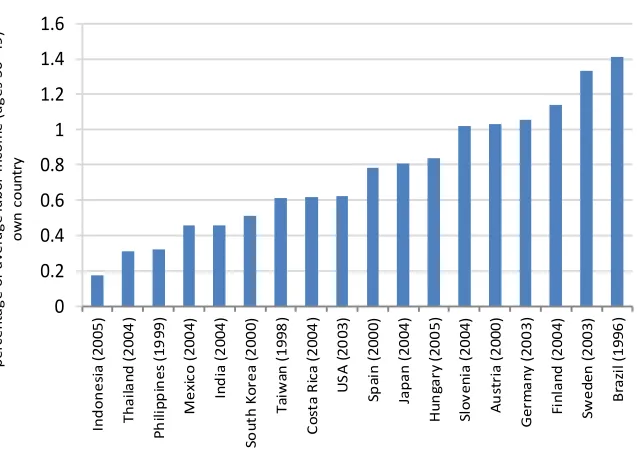
In short, the three countries analyzed represent different levels of development of the welfare state. As typically understood, Sweden has the largest size welfare state, while the United States and Spain have the smallest size among developed countries. This is confirmed by Figure 5, which shows the total size of welfare state transfers, measured as total transfers paid by the public sector in each country as a share of total labor income in the same country. For social and historical reasons the welfare state in Spain developed considerably later than the rest of Europe’s, mixing characteristics of different previously existing models on the continent (Esping-Andersen 1990).

Figure 5: Total size of the welfare state system (total public transfers to individuals as a share of total labor income)

(17)

4. Results: Decomposing the demographic dividend

This section presents and discusses the results. First, the data and methodology are described (a); second, the decomposition of the demographic dividend is performed for Spain, the United States, and Sweden (b); and finally, the impact of the structure of the public transfer system on the second demographic dividend is analyzed.

4.1 Data and methodology

We build a large-scale OLG model with realistic demography by single-year period and age. This type of model provides a useful tool for better understanding the interplay between demographics, economics, and intergenerational transfers. The model is standard in the sense that life cycle savings and consumption are endogenously determined by the agent, who decides how to distribute consumption over the life cycle. The main novelty comes from the explicit introduction of realistic private and public transfers taken from the NTA dataset, which allows for a thorough account of the impact of demography. Both per capita transfers and demographic information are exogenously given, while the tax level is scaled to guarantee a balanced government budget. We also introduce a mortality risk following Yaari’s (1965) approach (see Appendix A-1 for further details).

Following Bommier and Lee (2003) and Sánchez-Romero et al. (2013), we use realistic demography to better capture the interaction of demography and the economy. To make demographic information match a one-sex economic model, we reconstruct the population by single years of age for each country. Our reconstructions are based on historical records from the human mortality database (HMD 2014) and data from national statistical institutes from 1800 to 2010 (INE, several years, and Bureau of the Census 1949). From 2010 to 2050 we use Eurostat’s demographic assumptions for Spain and Sweden, and the UN Population Division for the United States. Before 1800 and after 2050, the vital rates are considered constant.

Agents are taxed both by a social security tax ( ), intended to pay retirement pensions, and an income tax ( ), intended to pay other government expenditures, consisting of in-kind transfers. Labor supply is perfectly inelastic and, hence, the introduced taxes do not affect it. Pensions are financed only by the income tax, while wages are subject to both income and social security taxes.16_{The per capita level of}

transfers is assumed to be constant, while taxes are adjusted to meet the two budget

16_{We also run simulations assuming that all taxes are levied on workers. However, this taxation scheme is}

(18)

constraints of the government on a PAYG basis. Finally, firms operate in competitive markets, so that wages and capital rents are equal to their net marginal product. Technology grows exogenously.

With the exceptions mentioned above, the model is standard. We assume a closed economy, which implies that factor prices (both wages and interest rate) are determined within the economy, depending mainly on the relative scarcity of capital and labor. Thereby, changes in population structure have a general equilibrium influence on factor prices, reinforced by changes in taxes needed to maintain the welfare state transfer system. Public expenditure in in-kind transfers is considered in the utility function (see Appendix A-1 for details). In turn, pension expenditure enters the budget constraint as a monetary transfer so that a negative impact on savings (crowding-out) can be expected.

(19)

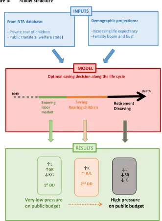
Figure 6: Model structure

Note: 1st_{DD and 2}nd_{DD are the first and second demographic dividends, respectively; L represents workers; K is capital; and SR is} the support ratio.

RESULTS

From NTA database:

- Private cost of children - Public transfers (welfare state)

Very low pressure High pressure

on public budget on public budget

↑L

↑SR

↓K/L

1st_DD

↑K ↑ K/L

2nd_DD

↓L

↓SR

↓ K Demographic projections:

-Increasing life expectancy -Fertility boom and bust INPUTS

Saving

Rearing children Retirement_Dissaving

Entering labor market

birth death

MODEL

(20)

Below we detail the data employed. The data on transfers from the NTA dataset is introduced as follows. From the net transfers shown in Figure 3 we use only the inflows (transfer receipts). Moreover, we distinguish between cash transfers (only pensions) and in-kind transfers (see Figure 7), which are modeled differently, as mentioned above.

Figure 7: Per capita age profiles of pensions and in-kind public transfers received by individuals

Regarding private transfers, as seen in Figure 3, the age pattern is quite similar in the three countries analyzed, especially with respect to transfers to the young. Interestingly, transfers to the old are negative, but since they are rather small, we ignore them for simplicity.

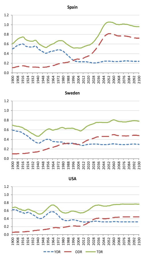
Finally, Figure 8 summarizes the demographic inputs by showing the evolution of the dependency ratio since 1900 in the three countries analyzed. Over the 20th_century,

the young dependency ratio (YDR) falls drastically, while the old dependency ratio (ODR) increases to a lesser extent. Demography in the 21st_{century is driven by the}

aging of baby boomers, the process being especially strong in Spain. Although Spanish dependency ratios were the lowest at the beginning of the period, both the ODR and total dependency ratios increase dramatically during the first part of the 21st_century

such that, at the end of the period, they are the highest. The YDR decreases to a lower figure in the case of Spain compared to the other two countries. The United States and Sweden show a similar pattern in the 21st_{century, with slightly higher old and total}

dependency ratios in the Swedish case.

0.00 0.10 0.20 0.30 0.40 0.50 0.60 0.70 0.80 0.90 1.00

0 5 10 15 20 25 30 35 40 45 50 55 60 65 70 75 80 85 90 age

In-kind transfers

SWE USA ESP

0.00 0.10 0.20 0.30 0.40 0.50 0.60 0.70 0.80 0.90 1.00

60 65 70 75 80 85 90

pe rc en ta ge of av er ag e la bo r in co m e (a ge s 30 ‒4 9) ow n co un tr y age Pensions

(21)

Figure 8: Past and future evolution of the dependency rate

Note: YDR = young dependency rate; ODR = old dependency rate; TDR = total dependency rate.

Source: Authors’ elaboration from HMD and Eurostat.

0.0 0.2 0.4 0.6 0.8 1.0 1.2 19 00 19 08 19 16 19 24 19 32 19 40 19 48 19 56 19 64 19 72 19 80 19 88 19 96 20 04 20 12 20 20 20 28 20 36 20 44 20 52 20 60 20 68 20 76 20 84 20 92 21 00 Spain 0.0 0.2 0.4 0.6 0.8 1.0 1.2 19 00 19 08 19 16 19 24 19 32 19 40 19 48 19 56 19 64 19 72 19 80 19 88 19 96 20 04 20 12 20 20 20 28 20 36 20 44 20 52 20 60 20 68 20 76 20 84 20 92 21 00 Sweden 0.0 0.2 0.4 0.6 0.8 1.0 1.2 19 00 19 08 19 16 19 24 19 32 19 40 19 48 19 56 19 64 19 72 19 80 19 88 19 96 20 04 20 12 20 20 20 28 20 36 20 44 20 52 20 60 20 68 20 76 20 84 20 92 21 00 USA

(22)

4.2 Decomposing the demographic dividend

The estimations of demographic dividends are presented below. Figure 9 shows the total growth rate of per capita income for the three countries during the 20th_{and 21}st

centuries. The increase in income due to the baby boom generation entering the labor market is clearly visible in all three cases. This positive effect occurs between 1970 and 2020, with a different time path and intensity in each country, and becomes negative ‒ note that it is detrended by the exogenous productivity growth rate ‒ when baby boomers retire. The Spanish baby boom shows the biggest effect, especially after the post-baby boom decline. It is important to note that the Spanish fertility rate is still far below replacement.

Figure 9: Total growth rate of per capita income

Note: Per capita income is measured in units of effective labor.

Source: Authors’ elaboration.

Given the sizable effect of demographics on the evolution of income per capita, it seems worthwhile to identify the different factors producing it. The model employed is designed to allow for this type of exercise. As explained in Section 2, we decompose the demographic dividend into three factors, as detailed in equation (6). In particular, the first demographic dividend is computed as the growth rate of the support ratio, making it possible to separate its two components: the purely demographic and the labor market age composition effect. The second demographic dividend is measured as

-1.5% -1.0% -0.5% 0.0% 0.5% 1.0% 1.5%

19

00

19

10

19

20

19

30

19

40

19

50

19

60

19

70

19

80

19

90

20

00

20

10

20

30

20

40

20

50

20

60

20

70

20

80

20

90

21

00

(23)

the growth rate of productivity, detrended by the exogenous productivity growth rate. Note that in this case, changes observed along the simulation refer to changes in per worker capital.

Figure 10 shows the decomposition proposed in equation (6) in the case of Spain. The growth rate of the strictly demographic support ratio (SRD_{) is negative from 1955 to}

1976, when baby boomers were born. It becomes positive from 1977 to around 2010, after these bigger cohorts enter the labor market. Subsequently, the growth rate of the support ratio becomes negative. The factor capturing the effect of demography on the labor market ‒ the ratio of effective producers to working-age population ‒ also has a sizable impact. This ratio only changes due to the age composition of the labor force. It increases from the end of the 1980s to the mid-2010s due to the higher relative size of cohorts in the most productive period of their life cycle (aged 30–55, see Figure 1) in the working population. This factor follows a path similar to the demographic support ratio, although it occurs a few years later. The second demographic dividend occurs during 2000–2040, while baby boomers accumulate savings, and disappears when all baby boomers are retired.

Figure 10: Decomposing the demographic dividend in Spain

Figure 11 shows the growth rate of the pure demographic support ratio (panel a) and the second demographic dividend (panel b) for the three countries analyzed. The main trends observed in Spain are reproduced in the other two countries, although with a different timeline and intensity. As shown in panel a), from the mid-20th_{century the}

increase in the growth rate of the pure demographic support ratio is primarily driven by

-1.5% -1.0% -0.5% 0.0% 0.5% 1.0% 1.5% 1 90 0 1 91 0 1 92 0 1 93 0 1 94 0 1 95 0 1 96 0 1 97 0 1 98 0 1 99 0 2 00 0 2 01 0 2 02 0 2 03 0 2 04 0 2 05 0 2 06 0 2 07 0 2 08 0 2 09 0 2 10 0

(24)

the baby boom. The highest increase occurs in the United States, followed by the Spanish baby boom, which is delayed more than a decade with respect to the other countries. Conversely, the growth rate of the pure demographic support ratio becomes negative around 2010, when baby boomers start retiring. In Spain, the decline lasts longer and is more pronounced because of the baby bust. In Sweden, the effects of the demographic transition are considerably smoother.

Figure 11’s panel b) shows that the second demographic dividend is less pronounced than the growth rate of the pure demographic support ratio. This is because the former incorporates economic adjustments from the general equilibrium model. As before, the second demographic dividend is delayed in the case of Spain. Nevertheless, it seems to be transitory for Spain and Sweden ‒ the area above the horizontal axis is almost the same as the area below it ‒ while it seems to be permanent for the United States.

Figure 11: Decomposing the demographic dividend

a) The growth rate of the pure demographic support ratio b) The second demographic dividend

Source: Authors’ elaboration.

Table 1 summarizes the results of our decomposition of the demographic dividend in each country for the period 1975–2100. These results, which complement those in Figure 11, are shown in 25-year periods to smooth short-term variations.

-1.5% -1.0% -0.5% 0.0% 0.5% 1.0% 1.5% 19 00 19 10 19 20 19 30 19 40 19 50 19 60 19 70 19 80 19 90 20 00 20 10 20 20 20 30 20 40 20 50 20 60 20 70 20 80 20 90 21 00

Spain USA Sweden -1.5% -1.0% -0.5% 0.0% 0.5% 1.0% 1.5% 19 00 19 10 19 20 19 30 19 40 19 50 19 60 19 70 19 80 19 90 20 00 20 10 20 20 20 30 20 40 20 50 20 60 20 70 20 80 20 90 21 00

(25)

Table 1: Evolution of the components of demographic dividends

N16-64/N EP/N16-64 1st DD 2nd DD, Y/EP Total DD

I II III IV V

Spain

1975‒2000 0.498 0.021 0.519 ‒0.122 0.397

2000‒2025 ‒0.165 0.030 ‒0.135 0.517 0.382

2025‒2050 ‒0.974 0.025 ‒0.950 0.095 ‒0.855

2050‒2075 0.067 ‒0.043 0.024 ‒0.351 ‒0.327

2075‒2100 0.111 ‒0.022 0.090 ‒0.032 0.058

1975‒2100 ‒0.094 0.002 ‒0.092 0.021 ‒0.071

United States

1975‒2000 0.249 0.337 0.586 0.053 0.638

2000‒2025 ‒0.234 ‒0.022 ‒0.257 0.335 0.079

2025‒2050 ‒0.091 0.014 ‒0.077 ‒0.082 ‒0.159

2050‒2075 ‒0.110 0.032 ‒0.078 ‒0.009 ‒0.087

2075‒2100 0.002 ‒0.003 ‒0.001 ‒0.022 ‒0.023

1975‒2100 ‒0.037 0.071 0.034 0.055 0.089

Sweden

1975‒2000 0.124 0.140 0.264 ‒0.117 0.147

2000‒2025 ‒0.262 ‒0.011 ‒0.274 0.213 ‒0.060

2025‒2050 ‒0.078 ‒0.039 ‒0.117 ‒0.116 ‒0.233

2050‒2075 ‒0.048 0.018 ‒0.029 ‒0.094 ‒0.123

2075‒2100 ‒0.048 0.018 ‒0.029 ‒0.094 ‒0.123

1975‒2100 ‒0.059 0.023 ‒0.035 ‒0.022 ‒0.057

Source: Authors' calculations. The numbers are average growth rates (%) for each period. N_(16-64)/N is the working age population to total population ratio, EP/N_(16-64) is the labor force (measured according to the NTA profile) to the working age population ratio, and Y/EP is the de-trended output per worker (in effective units).

1

We detrend the output by labor-augmenting technological progress that increases exogenously at an annual rate of 2%.

(26)

Major differences appear in the growth rate of the demographic support ratio, while differences in the labor market factor are lower. The high negative value in the third column for Spain in the period 2025–2050 reflects the strength of the baby bust in this country. Overall, for the entire period (1975–2100), the total change in the support ratio is negative in Spain and Sweden, and positive in the United States. Over the same period the total effect of changes in capital (column IV) is positive in Spain and the United States and negative in Sweden. Hence, the impact of population aging on economic growth in the United States is positive due to both the first and the second demographic dividend. In Sweden the opposite is true: Both effects are negative, mainly due to the size of public transfers. In the case of Spain the second demographic dividend is not large enough to offset the negative effect on the support ratio of population aging. Indeed, the strong baby bust creates an overall negative effect despite the positive effect of a limited welfare state.

4.3 Understanding the role of welfare state transfers

(27)

Figure 12: Counterfactual scenarios: Spain with different welfare state transfers

The first and second panels show the evolution of savings and capital in Spain compared to what they would have been if public transfers were as in Sweden or the United States. Looking first at the baseline, one can observe that the savings rate (defined as the ratio of total savings of the economy to net output) decreases while the baby boom generation is being born and recovers later, in the mid-1980s, when they start saving. Beginning in 2015 the savings rate starts falling again. The evolution of savings and the labor force translates into the evolution of capital in panel b). Capital (in effective units of labor) decreases slightly when baby boomers start entering the labor market and recovers as their savings start to be sizeable. As baby boomers retire it falls again, reaching a value somewhat higher than the 2000 value. Hence, the second demographic dividend almost disappears in Spain and has a limited permanent effect. This is due to the dissaving of baby boomers, together with the pressure of maintaining

1950 2000 2050 2100 2150 0

0.02 0.04 0.06 0.08 0.1 0.12 0.14 0.16 0.18

(a) Saving rate

19503 2000 2050 2100 2150 4

5 6 7

8 (b) Units of effective capital

19500 2000 2050 2100 2150 0.2

0.4 0.6 0.8

1 (c) Social Security tax

19500 2000 2050 2100 2150 0.2

0.4 0.6 0.8

1 (d) Income tax

(28)

the welfare state, which necessarily implies increasing taxes. This effect is clearly visible in panels c) and d), showing the evolution of the two taxes financing the pension system and the in-kind transfers system. The income tax financing in-kind transfers is affected both by the evolution of the YDR and ODR since these transfers nearly cover the two stages of dependency. It decreases with the fertility decline and recovers subsequently with the increase in transfers to the elderly due to the considerable increase in life expectancy and the higher number of retirees. The size of the social security tax is small at the beginning, when the ODR is still very low, but more than doubles due to increased life expectancy and, later, the retirement of baby boomers. The adjustment of the social security tax is also stronger because this tax is not levied on pensions, while the income tax is.

The changes observed with the counterfactual experiment are clear in the case of social security taxes (panel c) and income taxes (panel d). Note that in both cases the level reflects the different size of public transfers. First, the social security tax in the baseline is somewhere in between the tax resulting from introducing the Swedish and the United States transfers. This result directly follows from the level of pensions shown in Figure 7. Second, in the case of the income tax, Spain has the lowest value, which is consistent with the lower level of in-kind transfers.

The impact of the evolution of taxes on savings (panel a) and capital (panel b) illustrate that under the Swedish system, high levels of both cash and in-kind transfers ‒ especially old age transfers ‒ clearly reduce savings and especially capital over the entire period. From 2049 to 2061 the savings rate even becomes negative, as the savings of workers cannot compensate for the large dissaving of retired baby boomers. Under the United States transfer system, both savings and capital evolve similarly to the baseline, except for the period beginning around 2040. This suggests that the effect of a higher level of pensions in Spain is counterbalanced by the effect of a lower level of in-kind transfers.

(29)

Figure 13: Counterfactual scenarios: Spain with pensions of Sweden and the United States

Source: Authors’ elaboration.

Figure 14: Counterfactual scenarios: Spain with in-kind transfers of Sweden and the United States

Source: Authors’ elaboration.

19500 2000 2050 2100 2150 0.02

0.04 0.06 0.08 0.1 0.12 0.14 0.16

0.18 (a) Saving rate

19503 2000 2050 2100 2150 3.5

4 4.5 5 5.5 6 6.5 7 7.5

ESP baseline ESP-Pensions USA ESP-Pensions SWE

1950 2000 2050 2100 2150 0

0.02 0.04 0.06 0.08 0.1 0.12 0.14 0.16 0.18

(a) Saving rate

1950 2000 2050 2100 2150 3.5

4 4.5 5 5.5 6 6.5 7 7.5

(30)

Table 2 summarizes the total impact of welfare state transfers on the demographic dividend, again in 25-year periods. Columns I‒III show the first demographic dividend and its decomposition, which remain unchanged with respect to the results in Table 1. Column IV indicates the second demographic dividend on the Spanish baseline, compared to the case in which the United States’ and Sweden’s public transfers are introduced. In both scenarios, the figures are lower. This is particularly the case when public Swedish transfers are introduced, as the combination of the drastic Spanish aging process and the high level of Swedish welfare state transfers reduces capital to a greater extent and, for the entire 1975–2100 period, the effect on capital per worker becomes negative.

Table 2: Evolution of Spanish demographic dividend with different welfare state transfers

N16-64/N EP/N16-64 1st DD 2nd DD, Y/EP Total DD

I II III IV V

Spain (baseline)

1975‒2000 0.498 0.021 0.519 ‒0.122 0.397

2000‒2025 ‒0.165 0.030 ‒0.135 0.517 0.382

2025‒2050 ‒0.974 0.025 ‒0.950 0.095 ‒0.855

2050‒2075 0.067 ‒0.043 0.024 ‒0.351 ‒0.327

2075‒2100 0.111 ‒0.022 0.090 ‒0.032 0.058

1975‒2100 ‒0.094 0.002 ‒0.092 0.021 ‒0.071

Spain (with United States transfers)

1975‒2000 0.498 0.021 0.519 ‒0.118 0.401

2000‒2025 ‒0.165 0.030 ‒0.135 0.516 0.381

2025‒2050 ‒0.974 0.025 ‒0.950 0.070 ‒0.880

2050‒2075 0.067 ‒0.043 0.024 ‒0.410 ‒0.386

2075‒2100 0.111 ‒0.022 0.090 ‒0.058 0.032

1975‒2100 ‒0.094 0.002 ‒0.092 0.000 ‒0.092

Spain (with Sweden transfers)

1975‒2000 0.498 0.021 0.519 ‒0.220 0.299

2000‒2025 ‒0.165 0.030 ‒0.135 0.471 0.336

2025‒2050 ‒0.974 0.025 ‒0.950 0.020 ‒0.929

2050‒2075 0.067 ‒0.043 0.024 ‒0.593 ‒0.569

2075‒2100 0.111 ‒0.022 0.090 ‒0.065 0.024

1975‒2100 ‒0.094 0.002 ‒0.092 ‒0.078 ‒0.170

Source: Authors' calculations. The numbers are average growth rates (%) for each period. N_(16-64)/N is the working age population to total population ratio, EP/N_(16-64) is the labor force (measured according to the NTA profile) to the working age population ratio, and Y/EP is the de-trended output per worker (in effective units).

(31)

In summary, our results show that the implementation of the transfer systems of the United States or Sweden in the Spanish economy would lead to higher negative impacts of population aging. This is especially true for the Swedish system, where, as seen in Figure 12, the final level of capital once baby boomers disappear is notoriously lower than the initial value. These results have important implications for welfare state reforms in the face of demographic aging.

5. Discussion and conclusions

Attempts have been made, from different perspectives, to measure the effects of demographics on economic growth. These effects can be positive or negative. In fact, the first demographic dividend, occurring when the baby boom generation is part of the labor force, reverts as this generation retires and increases the demand for public transfers. Indeed, when baby boomers approach retirement age in developed countries, greater pressure is placed on welfare state transfers, which are mainly financed on a PAYG basis. In this context, it seems clear that the margin for reforms of the welfare state depends on the size and timeline of demographic dividends.

In this paper we have decomposed the demographic dividend using a model that permits us to investigate the joint effects of demographic change and welfare state transfers on savings and capital accumulation. The growth rate of per capita income is broken down into three terms. The first term is the purely demographic support ratio. The second term isolates the age composition effect of the labor market. Finally, the third term collects the increase in income per worker due to changes in capital intensity (baby boomers saving/dissaving).

(32)

Furthermore, by isolating the effect of demography and welfare state transfers in the counterfactual scenarios, we observe that an extension of welfare state transfers in Spain toward Nordic standards would eliminate the permanent effects of the second demographic dividend. Note that the Spanish Mediterranean welfare state is a version of the European welfare state model halfway between the continental and the Nordic model. Nevertheless, the positive side of our results is that although the first demographic dividend has already disappeared in Spain (and in most other developed countries), the second demographic dividend can still last for a couple of decades, giving some margin for reform.

In any case, our results should be interpreted with caution since they are affected by the way in which welfare state transfers are modeled. There are many aspects of current welfare states that cannot be modeled in detail in this framework. Note that our representative agent approach does not consider the equity–efficiency tradeoff for welfare state transfers. Deriving definite conclusions on the impact of transfers on the welfare of agents requires further research on the feedback effects between public and private transfer systems and demographic transition. In fact, the way in which the government intervenes on intergenerational transfers and its impact on fertility remains an unanswered issue in the literature. Additionally, further investigation is needed to identify the role of education transition on the demographic dividend.

6. Acknowledgements

(33)

References

Arellano, M. and Bond, S. (1991). Some tests of specification for panel data: Monte Carlo evidence and an application to employment equations. Review of

Economic Studies 58(2): 277–297.doi:10.2307/2297968.

Bloom, D.E. and Williamson, J.G. (1998). Demographic transitions and economic miracles in emerging Asia.The World Bank Economic Review 12(3): 340–375.

doi:10.1093/wber/12.3.419.

Bommier, A. and Lee, R. (2003). Overlapping generations models with realistic demography. Journal of Population Economics 16(1): 135–160. doi:10.1007/ s001480100102.

Braun, A.R., Ikeda, D., and Jones, D.H. (2009). The saving rate in Japan: Why it has fallen and why it will remain low.International Economic Review 50(1): 291– 321.doi:10.1111/j.1468-2354.2008.00531.x.

Bureau of the Census (1949). Historical statistics of the United States, 1789–1945. Washington, D.C.: US Government Printing Office.

Chen, K., Imrohoroğlu, A., and Imrohoroğlu, S. (2006). The Japanese saving rate. The

American Economic Review96(5): 1850–1858.doi:10.1257/aer.96.5.1850.

Chen, K., Imrohoroğlu, A., and Imrohoroğlu, S. (2007). The Japanese saving rate between 1960 and 2000: Productivity, policy changes, and demographics.

Economic Theory 32(1): 87–104.doi:10.1007/s00199-006-0200-9.

Crespo-Cuaresma, J., Lutz, W., and Sanderson, W.C. (2014). Is the demographic dividend an education dividend?Demography 51(1): 299–315. doi:10.1007/s13 524-013-0245-x.

Cutler, D., Poterba, J., Sheiner, L., and Summers, L. (1990). An ageing society: Opportunity or challenge. Brookings Papers on Economic Activity 1: 1–74.

doi:10.2307/2534525.

Esping-Andersen, G. (1990). The three worlds of welfare capitalism. New Jersey: Princeton University Press.

Feyrer, J. (2007). Demographics and productivity. The Review of Economics and

Statistics 89(1): 100–109.doi:10.1162/rest.89.1.100.

HMD (2014). Human Mortality Database [electronic resource]. Berkeley: University of California and Germany: Max Planck Institute for Demography Research.

(34)

INE (1857–1970). INEbase, Censos de Población del período 1857–1970 [electronic resource]. Madrid: Instituto Nacional de Estadística. http://www.ine.es/ine baseweb/71807.do?language=0.

INE (1981, 1991, 2001, and 2011). INEbase, Censos de Población y Viviendas [electronic resource]. Madrid: Instituto Nacional de Estadística.http://www.ine. es/censos2011_datos/cen11_datos_inicio.htm.

Kelley, A.C. and Schmidt, R.M. (2005). Saving dependency and development.Journal

of Population Economics 9(4): 365–386.doi:10.1007/BF00573070.

Klump, R. and De La Grandville, O. (2000). Economic growth and the elasticity of substitution: Two theorems and some suggestions. The American Economic

Review 90(1): 282–291.doi:10.1257/aer.90.1.282.

Lee, R. and Mason, A. (2011). Population ageing and the generational economy: A

global perspective. Northampton: Edward Elgar.doi:10.4337/9780857930583.

Lee, R., Mason, A., and Miller, T. (2000). Life cycle saving and the demographic transition: The case of Taiwan. Population and Development Review26: 194– 219.

Lee, R., Mason, A., and Miller, T. (2001). Saving, wealth, and the demographic transition in East Asia. In: Mason, A. (ed.). Population change and economic

development: Challenges met, opportunities seized. Stanford: Stanford

University Press: 155–184.

Lee, R., Mason, A., and Miller, T. (2003). Saving, wealth and the transition from transfers to individual responsibility: The cases of Taiwan and the United States.

The Scandinavian Journal of Economics 105(3): 339–357.

doi:10.1111/1467-9442.t01-2-00002.

Lutz, W., Crespo-Cuaresma, J., and Sanderson, W.C. (2008). The demography of educational attainment and economic growth. Science 319(5866): 1047–1048.

doi:10.1126/science.1151753.

Mason, A. (2005). Demographic transition and demographic dividends in developed

and developing countries. United Nations expert group meeting on social and

economic implications of changing population age structure, Mexico, July 28, 2005.

Mason, A. and Lee, R. (2006). Reform and support systems for the elderly in developing countries: Capturing the second demographic dividend. Genus

(35)

Miyagiwa, K. and Papageorgiou, C. (2003). Elasticity of substitution and growth: Normalized CES in the Diamond model. Economic Theory 21(1): 155–165.

doi:10.1007/s00199-002-0268-9.

Murray, M.P. (1994). How inefficient are multiple in-kind transfers?Economic Inquiry

32(2): 209–227.doi:10.1111/j.1465-7295.1994.tb01325.x.

Patxot, C., Rentería, E., Sánchez-Romero, M., and Souto, G. (2011). Results for GA and NTA: The sustainability of the welfare state in Spain. Moneda y Crédito

231: 7–51.

Prskawetz, A. and Sambt, J. (2014). Economic support ratios and the demographic dividend in Europe. Demographic Research 30(34): 963–1010. doi:10.4054/ DemRes.2014.30.34.

Roodman, D. (2009). A note on the theme of too many instruments.Oxford Bulletin of

Economics and Statistics 71(1): 135–158. doi:10.1111/j.1468-0084.2008.005

42.x.

Sánchez-Romero, M. (2013). The role of demography on per capita output growth and saving rates. Journal of Population Economics 26(4): 1347–1377. doi:10.1007/ s00148-012-0447-3.

Sánchez-Romero, M., Patxot, C., Rentería, E., and Souto, G. (2013). On the effects of public and private transfers on capital accumulation: Some lessons from the NTA aggregates. Journal of Population Economics 26(4): 1409–1430.

doi:10.1007/s00148-012-0447-3.

United Nations (2013). National Transfer Accounts manual: Measuring and analyzing the generational economy. New York: United Nations Population Division, Department of Economic and Social Affairs.

Williamson, J.G. (2013). Demographic dividends revisited.Asian Development Review

30(2): 1–25.doi:10.1162/ADEV_a_00013.

Yaari, M. (1965). Uncertain lifetime, life insurance and the theory of the consumer.

(36)

Appendix: Modeling approach and sensitivity analysis

A-1. The model

Below we describe the special features of the model, detailing the equations that deviate from the standard specifications. We employ a large-scale OLG model with individuals living from age 0 to a maximum of 110 years. Agents start making economic decisions when they reach 21 years old. Before that age, their consumption is decided by the household head. Individuals face mortality risk in every period of their life. To highlight the effects of mortality, the mortality risk is considered in the utility function as in Yaari (1965). Households derive utility from both private and public consumption according to the following expected utility function:

= ∑ ( , , ) (A-1)

wherex is the age of the household head,Ω is the maximum lifespan,c stands for total household consumption (public and private), is public consumption, and stands for the number of equivalent adult consumers in the household. The time subscripts are omitted for simplicity. The discount factor is composed of time preference (reflected in

) and survival probability ( ).

The instantaneous utility function, based on Murray (1994), takes the following functional form:

; ,γ = γ _γ − 1 (A-2)

whereσ is the relative risk aversion coefficient. Note that the parameter (number of equivalent adult consumers) increases utility once the household consumption is adjusted in per capita terms. This way, we assume that adults make decisions for their own well-being as well as for their dependent children, following Lee, Mason, and Miller (2000). In any other respect there is no altruism. The utility function implies that unexpected bequests might arise from deceased individuals without intentional bequest motives. For simplicity, bequests are collected by the government, easing the budget constraint.

The budget constraint faced by a household head is as follows:

(37)

for x=0, … ,Ω

= 0

≥ 0 (A-3)

w being the wage, and the social security and income taxes, p the pension benefits received from the social security system, a the assets, and r the interest rate. Note that gross labor income is first levied by social contributions, and the resulting net amount is then subject to an income tax levy, while pensions are subject only to the income tax levy.

Households maximize the utility function in (A-1) given (A-2) subject to the budget constraint (A-3) with respect to total consumption, cx. The Euler equation

resulting from the first order conditions of the household problem is given by:

= (1 + )

The representative firm operates with a constant elasticity of substitution technology,

= , = + (1 − ) (A-4)

whereH = AL,A being the labor-augmenting technological progress, which is assumed to grow at an exogenous constant rate of 2% in all countries for comparability reasons,

L the labor force (measured using the NTA labor income profile),K physical capital,α

the capital share, andλ the elasticity of substitution between the production factors. The following two equations define the government budget constraint. The first stands for the social security pensions system and the second for in-kind transfers. We assume a defined benefit pensions system, adjusting the social contribution rate in each period in a PAYG manner. The same happens in the other equation, where we also assume PAYG financing, so that the government does not accumulate debt.

(38)

= (1 − ) + + (A-6)

whereG stands for total in-kind government expenditure,P andp for the total and per capita pensions, and B is the total annual accidental bequests, which are levied at a 100% tax rate by the government.

A-2. Parameter values and sensitivity analysis

In this section we provide a sensitivity analysis with respect to some of the parameters used in our calibration. Table A-1 shows the parameter values assumed in our results. The values chosen are standard in literature, which allows us to focus on the long-term impact of demography in the three analyzed countries.

In the case of the elasticity of substitution between production factors (µ), we set a value of 1.2 in the baseline model. Klump and De La Grandville (2000) show that a higher elasticity of substitution between production factors implies an increase in income and capital share. However, the relationship between factor substitutability and economic growth is not monotonic in OLG models, as shown by Miyagiwa and Papageorgiou (2003). To see the economic effects the elasticity of substitution has on our results, we run simulations with two alternative µ values for each country (see Table A-2). We set µ at 1.0 and at 0.8. Note that a value of µ at 1.0 corresponds to a Cobb-Douglas production function. Values of µ above (below) one imply that the share of labor on output decreases (increases) as the capital-to-output ratio rises (falls). Recall that: _ℎ _{= 1 − ( / )} . Therefore, as public expenditures are assumed to be financed by income taxes, the government needs to raise the income tax rate when higher µ values are assumed (see the last column in Table A-2).

Table A-2 also shows the effect of different values of µ on demographic dividends. The impact of different elasticities of substitution between input factors on the growth rate of output per worker is shown in the fourth column. Note that all values in the table are expressed in percentage points. In principle, given an effective capital per worker higher than one, the growth rate of output per worker is greater the higher the elasticity of substitution between input factors. Indeed, after some manipulations of our CES production function, we can derive that the growth rate of output per worker is:

= · 1 + (1 − ) − 1 (A-7)

(39)

This result holds for the cases of Spain and the United States. In Sweden, the effect of µ on the growth rate of output per worker is reversed because the supply of capital by households is very inelastic due to the high taxation rates. In any case, the values of annual average growth rates displayed in Table A-2 are similar for the different values of µ.

Table A-3 shows the differential effect of alternative risk aversion coefficients on the first and second demographic dividends. The baseline value is σ = 2, and we obtain results with an alternative coefficient of σ = 1. Comparing the two scenarios, we can conclude that our results are robust to changes in the risk aversion coefficient. The biggest discrepancy can be observed in Sweden, which is caused by the increase in the elasticity of capital supply.

Table A-1: Calibration parameters

Parameter Symbol Calibration value

Annual productivity growth rate g 0.02 Elasticity of substitution between production factors µ 1.20

Capital share in income α 0.33

Capital depreciation rate δ 0.05

Relative risk aversion (in utility) σ 2.00

Discount factor (in utility) β 0.99

Table A-2: Annual average growth rates by country and elasticity between input factors, 1975–2100 (%) (productivity detrended values)

Country

Elasticity of substitution between input

factors

1st_DD ₂nd_DD _{Total effect} on (Y/N)