EXTERNAL ADJUSTMENT WITH
A COMMON CURRENCY: THE CASE
OF THE EURO AREA
Alberto Fuertes
Documentos de Trabajo
N.º 1936
Documentos de Trabajo. N.º 1936
2019
(*) The views in this paper are those of the author and do not represent the views of the Banco de España or the Eurosystem.
(**) E-mail: [email protected] Alberto Fuertes (**)
BANCO DE ESPAÑA
EXTERNAL ADJUSTMENT WITH A COMMON CURRENCY:
The Working Paper Series seeks to disseminate original research in economics and fi nance. All papers have been anonymously refereed. By publishing these papers, the Banco de España aims to contribute to economic analysis and, in particular, to knowledge of the Spanish economy and its international environment.
The opinions and analyses in the Working Paper Series are the responsibility of the authors and, therefore, do not necessarily coincide with those of the Banco de España or the Eurosystem.
The Banco de España disseminates its main reports and most of its publications via the Internet at the following website: http://www.bde.es.
Reproduction for educational and non-commercial purposes is permitted provided that the source is acknowledged.
© BANCO DE ESPAÑA, Madrid, 2019
Abstract
This paper analyzes the behaviour of the external adjustment path for the four main economies in the euro area. I fi nd a structural break in the behaviour of the net external position at the time of the introduction of the euro for France, Italy and Spain, pointing out that the inception of the common currency changed their external adjustment process. Germany does not show this structural break, being its external position more affected by other events such as the country reunifi cation in 1989. I also fi nd that France and Italy will adjust the net external position mainly through the valuation component, while Germany and Spain will restore their external balance mostly through the trade component. The common currency area could have exacerbated Germany’s net creditor position as the evolution of the euro has reacted to the external adjustment needs of debtor countries such as Italy and Spain.
Keywords: external adjustment, exchange rate regime, structural breaks, valuation adjustment.
Resumen
Este trabajo analiza el comportamiento de la posición fi nanciera externa de las cuatro principales economías de la zona del euro, y si la introducción de la moneda única ha modifi cado su evolución. Se documenta una ruptura estructural en el comportamiento de la posición externa neta de Francia, Italia y España en el momento de la introducción del euro, que señala que la creación de la moneda única cambió el proceso de ajuste externo en estos países. Alemania, sin embargo, no experimentó esta ruptura estructural y su posición externa se ha visto más afectada por otros eventos, como la reunifi cación del país en 1989. Los resultados empíricos muestran que Francia e Italia ajustarán sus desequilibrios externos principalmente por medio del componente de valoración, mientras que en Alemania y España primará el componente de comercio. El área monetaria común puede haber fomentado el incremento en la posición acreedora de Alemania, ya que el comportamiento de la moneda única ha estado condicionado por las necesidades de ajuste externo de países deudores como Italia y España.
Palabras clave: ajuste externo, régimen de tipo de cambio, cambio estructural, componente de valoración.
1The U.S., for instance, had a negative IIP representing 39% of its GDP at the end of 2017.
2In absolute terms Spain holds the second largest net external debtor position in the world amounting
941.507 billion euros (1.108.386 billion dollars). The US is the country with the largest negative net external position totaling 7.725.002 billion dollars.
1
Introduction
liabilities denominated in different currencies (valuation component) and also of affecting
future net exports (trade component). Lane and Shambaugh (2010) do also emphasize the
impact of currency movements on the external positions for a large sample of countries. They
find that the wealth effects associated with exchange rate changes are substantial and can explain a sizeable share of the overall valuation shocks that hit the net foreign asset position.
Moreover, Fuertes (2019) shows the importance of the nominal exchange rate regime for the
process of external adjustment in the US. He finds that the collapse of the Bretton Woods The process of external adjustment within a common currency area has received little
at-tention in the literature, despite the fact that an important mechanism of correction of
imbalances, the nominal exchange rate, has been partially cancelled. The lack of nominal
exchange rate adjustment for the bilateral transactions and external positions among the
countries of the currency area may difficult the reduction of large net external liability
posi-tions. As an alternative, the more complicated and slower process of adjustment in product
prices and wages (internal devaluation) may operate in the absence of the nominal foreign ex-change. Keeping the net external position under control is crucial given that economies with
large net liability positions are more vulnerable to capital markets disruptions and growing
imbalances may trigger sustainability problems. These vulnerabilities were evident during
the global financial crisis and the subsequent euro area crisis, as several economies
experi-enced sudden stops, sovereign debt problems, or both. Moreover, recent research by Gadea
et al. (2018) shows how external imbalances also affect the business cycle, as economies with
large external imbalances experience slower recoveries.
At the end of 2017 the international investment position (IIP) of the euro area, the largest
common currency union in the world, recorded a net liability position of 388 billion euros,
representing 3.5% of its GDP. Even though this is almost a balanced position1 there are large
differences among countries, which have become even larger after the inception the euro in
1999. For instance Germany amounts a net external creditor position representing 59% of
its GDP at the end of 2017 while Spain shows a net debtor position representing 81% of its GDP2. Peripheral countries face the largest net liabilities positions in the euro area, with
Portugal, Greece and Ireland showing net external positions representing 105.8%, 140.9%
and 148.3% of its GDP respectively (see Chart 1).
The process of external adjustment for the countries within the euro area is different because these economies share a common currency. Gourinchas and Rey (2007) show that the
dy-namics of the exchange rate play a major role in the external adjustment process of the US
3There may be second order effects as the depreciation could affect the terms of trade with the countries
outside the currency area.
system of fixed exchange rates in 1973 affected the behaviour of the US net external
posi-tion, implying an increase in the importance of the valuation component during the floating
period. Given all the previous empirical evidence, it is expected that the inception of the
common currency may have affected the external adjustment process for the countries of the
euro area.
The introduction of the euro made the effects of nominal exchange rate changes to disappear
among the countries in the currency area. First, a net debtor country could not rely anymore
on foreign exchange depreciations to reduce the relative value of the local currency external
debt held with other countries of the currency union. Similarly, a currency depreciation will
not have any direct impact on the bilateral trade among the countries with the same currency
3. Second, the behaviour of the exchange rate may not favour the external adjustment
of all countries in the currency area, as foreign exchange movements will respond to the
macroeconomic and monetary conditions of the whole currency union. For instance, a debtor
country within the union that would benefit from an exchange rate depreciation to improve
its external position may face an appreciating currency due to the macroeconomic situation
of the other countries and the current monetary policy of the central bank. Because of these
two reasons, changing from a floating to a fixed exchange rate regime within a common
currency area may difficult the external adjustment and could be potentially dangerous for
countries with large negative external positions. Understanding how the external adjustment
process has evolved over time for the countries of the euro area and the implications of the introduction of the euro for that process are the main research questions of the paper.
This work is related to the studies analyzing the external adjustment process, with an
em-phasis on the relevance of valuation effects and the nominal exchange rate regime. Friedman
(1953) initiated the debate arguing that flexible exchange rates facilitate the correction of external imbalances by allowing an automatic adjustment in a context of nominal rigidities.
Following this idea several studies have analyzed empirically the validity of this assumption
by investigating how current account imbalances are corrected depending on the exchange
rate regime. Gosh et al. (2014) find a robust relationship between the exchange rate regime
and the speed of external adjustment confirming Friedman´s hypothesis. Similarly,
Eguren-Martin (2016) finds evidence that flexible exchange rate arrangements deliver faster current
account adjustment among non-industrial countries. Fuertes (2019) focuses on the conse-quences of a change in the exchange rate regime for the behaviour of the net external position,
being the first study to analyze the adjustment of the net external imbalance instead of only
focusing on the current account. He finds that the behaviour of the U.S. net external position
changed at the end of the Bretton Woods system of fixed exchange rates in 1973, with the
U.S. external imbalance increasing its variance and turning into a debtor position during
adjustment process mainly through the valuation channel, which increased its relevance over
the floating period. Previously, Gourinchas and Rey (2007) had already documented the
importance of the valuation component for the external adjustment process, finding that
this component explained 27% of the variance for the cyclical part of the US net external
position. Further analysis by Evans and Fuertes (2011) and Evans (2012) show that the contribution to the external adjustment of the valuation component is larger than that of
the trade component when analyzing the whole U.S. external imbalance and not only its
cyclical part. Theoretical models have also emphasized the role of valuation effects on the
dynamics of the net external position. Devereux and Sutherland (2010) present a DSGE
model with portfolio choice capable to reproduce the dynamics of the valuation channel of
external adjustment. The model can only generate unexpected valuation effects, being the
anticipated ones small and reproduced at higher orders of approximation. Ghironi et al.
(2015) also examine the valuation channel of external adjustment theoretically in a DSGE
model, being able to separate asset prices and quantities in the definition of net foreign assets. This is more consistent with previous empirical work that has documented the relevance of
expected valuation effects (see Gourinchas and Rey (2007), Evans and Fuertes (2011) and
Evans (2012)).
In this paper I analyze the external adjustment path of the four main economies of the euro area, covering both the period before and after the introduction of the euro, to understand
how the currency area affected the external adjustment process. In principle, the
incep-tion of the euro should have limited the capacity of the nominal exchange rate to correct
external imbalances. This is evident as most of the research related to the correction of
external imbalances in euro area countries has focused on the process of internal devaluation
and its consequences, acknowledging the limited role of the nominal exchange rate.
Differ-ent studies have analyzed theoretically and empirically how currDiffer-ent account deficits should be transformed into surpluses by a combination of a decrease in domestic spending, real
exchange rate depreciation and a reduction in unit labor costs4.
To the best of my knowledge this is the first attempt to study the behaviour of the net
external position for a set of euro area countries, including debtor and creditor countries, and analyzing the implications of the common currency area for their external adjustment
paths. Within this framework the main contributions of the paper are the following: First
I build a novel data set of quarterly positions on assets and liabilities for the categories of
equity, fixed income, direct investment and other assets/liabilities for France, Germany, Italy
and Spain. The data set also includes estimates of quarterly total returns and capital gains
for each of those categories. Second, I find a structural break in the behaviour of the net
external position for France, Italy and Spain at the time of the introduction of the euro,
pointing out that the inception of the common currency changed the external adjustment
4See for example Atoyan et al. (2013), Kang and Shambaugh (2014), Eggertsson et al. (2013) or Andr´es
process. The fact that Germany does not show this structural break is consistent with
the exchange rate regime mainly affecting the valuation channel of external adjustment,
given that the variance of Germany’s net external position is almost completely explained
by the trade channel. I also find a structural break for the external imbalances of Spain
and Italy during the crisis of the European Exchange Mechanism (ERM) in 1992. Over
this period the Italian lira and the Spanish peseta were devaluated and Italy abandoned
the ERM. The importance of the valuation component of external adjustment increases after the introduction of the euro for France and Italy, and decreases for Germany and
Spain. Third, I also find that France and Italy will adjust the net external position mainly
through the valuation component of external adjustment, while Germany and Spain will
restore their external balance mostly through the trade component. Both the valuation and
trade components have supported the evolution of the net external position in France, Italy
and Spain. In the case of Germany the valuation component has limited the overall trend
towards a larger creditor position, which has been driven by the trade component. Fourth,
in the absence of unexpected shocks, the half-live of the external imbalances is relatively
short as Germany and Spain, the two countries with the largest imbalances, will be able to reduce their creditor and debtor positions by half in 7 and 3 years respectively. Finally, I
documented asset pricing implications as the net external position has explanatory power
over the future evolution of the exchange rate. A deterioration in the external imbalance of
France, Italy and Spain implies a future depreciation of the euro, facilitating the external
adjustment through the trade component. On the contrary, for Germany, the behaviour of
2
Data
The data set includes information for France, Germany, Italy and Spain about their
inter-national investment position (IIP) as well as the external portfolio returns for assets and
liabilities each period. The IIP data comes from the Balance of Payments Statistics (BOPS)
of the IMF. Using the original data I obtain asset and liabilities positions for different
cat-egories: equity, direct investment, fixed income and other assets/liabilities. The data set is
constructed following the same methodology employed by Gourinchas and Rey (2007). The IIP data from the BOPS comes on a quarterly frequency only for the more recent years and
I estimate quarterly positions using portfolio flows and total returns to increase the sample the common currency has hindered the external adjustment as it has supported the increase
in its creditor position.
The paper proceeds as follows: Section 2 presents the data set. Section 3 includes most of
the empirical analysis, including the structural break tests, the estimation of the valuation and trade components and asset pricing implications. Section 4 develops robustness checks
period 5 . It is important that the data set include the years before and after the inception
of the euro in order to fully characterise the changes triggered by the introduction of the
common currency.
The other important part of the data set are the portfolio returns. The returns are
com-puted from market prices for each of the asset/liabilities classes: equity, direct investment,
fixed income and other assets/liabilities. In order to identify the market weights within
the categories of equity, direct investment and fixed income6 I use the Coordinated Direct
Investment Survey (CDIS) and the Coordinated Portfolio Investment Survey (CPIS), both
from the IMF. Once I have the market weights for each quarter and asset category I calculate
total returns and capital gains for each market and compute the total portfolio return for the different categories using the market weights. For example, for the equity assets
cate-gory, I get from the CPIS the value of equity assets held in each foreign country to obtain
5The data availability of the IIP at the quarterly and yearly frequency is different for each country, with
the final estimated quarterly samples spanning from 1980: IV to 2017: I for Germany, Italy and Spain. For France the sample begins on 1989:III.
6For “other assets” I use the same market weights as those computed for short-term fixed income assets.
For “other liabilities” I assume the total value is denominated in local currency using the same returns as those from short term fixed income liabilities.
geographical weights that will be used together with the returns of the corresponding
bench-mark equity index to compute the total return. The information contained in the bench-market
weights is also important because we can assess the portfolio value of the positions held with
the other countries of the currency area. Chart 2 shows the percentage of foreign equity assets held in euro area countries for the four countries of analysis. As we can see all of them
hold a relevant share of their equity assets portfolio in the euro area. Even though there
is no information about euro area equity weights before 2001 it is reasonable to think that
the introduction of the common currency may have changed the behaviour of capital gains.
Before the introduction of the euro capital gains were determined both by asset prices and
foreign exchange movements. After the introduction of the euro much of the capital gains
coming from the equity assets portfolio were not affected by nominal exchange rate changes,
being mainly determined by asset price changes7. This may have also affected the size and
direction of external wealth effects, modifying the behaviour of the valuation channel of
external adjustment.
I complete the data set with information on imports and exports for each country8. We can
asses the relevance of the commercial ties the four countries of analysis have with the rest
of the euro area members. Chart 3 shows the share of imports plus exports traded with
the rest of euro area countries. The four countries show shares over 40%, with a slightly declining trend over the last years. It is noticeable the large increase experienced by Spanish
imports and exports since 1986, the year Spain joined the European Union. The large share
7The other asset classes (FDI, fixed income and other assets) do also show a large share of euro area
positions after the introduction of the common currency.
of bilateral trade of the four countries with the rest of the euro area shows the potential
impact that the common currency may have induced to the evolution of the net external
imbalance, in this case through the trade channel of external adjustment.
Finally, Table 1 shows the estimates of real portfolio returns for assets and liabilities as well
as the return differentials. The table includes real returns for the complete sample as well
as for the periods before and after the introduction of the euro. The only country able to
obtain an average positive return differential over the whole period was Germany, with the
other countries experiencing, on average, larger returns on their foreign liabilities than on
their foreign assets. During the period after the introduction of the euro Spain was able to
generate positive return differentials on average, while the other countries presented negative return differentials. The reduction of financing costs due to joining the euro area may have
influenced the positive return differential obtained by Spain.
In order to analyze the external adjustment process of a country Evans and Fuertes (2011)
derive the present value relation for the net external position using several log-linearizations
that include assumptions about the behaviour of different financial ratios9. I will next
summarize the main steps to obtain this present value equation, which will be used as the
starting point for the empirical analysis.
I start with the following equation:10
F At−F Lt≡Xt−Mt+RtF AF At−1−RF Lt F Lt−1 (1)
9See Evans and Fuertes (2011) and Fuertes (2019)
10The analysis does not include the secondary income which has been historically low for the four countries.
3
Empirical analysis
Where F AtandF Lt are gross foreign assets and liabilities at the end of periodt, Xt andMt are exports and imports during period t, all measured in terms of the consumption index.
RF At andRF Lt represent gross real returns on foreign assets and liabilities between the end of periods t−1 and t. After several log-linearizations and some algebra I obtain the following relation:
nf at ≈rtNF A+ 1−ρ
ρ nxt−1+
1
ρnf at−1 (2)
Where nf at is the log of the ratio of foreign assets to liabilities at the beginning of period t. rtNF A is the log of the return differential of foreign assets and liabilities and nxt is the difference of the log of exports minus imports. ρ is a discount factor. Defining nxat =
nf at+nxt and Δnxt =nxt−nxt−1 I obtain the following expression:
nxat≈rNF At + Δnxt+1
I impose the no-Ponzi game condition Etlimi→∞ρi(nxat+i) = 0 on the equation above to rule out the possibility that a country defaults on its foreign claims. The next equation
shows the present value relation between the variable nxat and future expected portfolio
where t is a vector of zero mean errors. The VAR has the following first order companion representation:
Zt = ¯AZt−1+ ¯t
11In deriving equation (4) I have performed several first order approximations. To assess the accuracy of
those approximations we can compute the error term from equation (3) which also includes any measurement errors from the original data. The error term is small and stationary for the four countries under analysis Iterating forward equation (3) and taking expectations conditioned on periodt information,
which includes de value of nxat , I obtain:
nxat≈ −Et ∞
i=1
ρi(rtNF A+i + Δnxt+i) +Et lim i→∞ρ
i(nxa t+i)
return differentials and net exports growth,11
nxat≈ −Et ∞
i=1
ρi(rNF At+i + Δnxt+i) (4)
I will use nxat as the variable of interest that measures external imbalances, being the two terms at the right hand side of the equation the valuation component and the trade
compo-nent respectively. This equation shows how current imbalances will be corrected in the future.
Equation (4) implies that the net external position can only vary if it forecasts changes in
portfolio returns or if it forecasts changes in net exports growth. If Et∞i=1ρirtNF A+i = 0, any adjustment of the net external position will come from future changes in net exports growth
(trade component). On the other hand, if Et∞i=1ρiΔnxt+i = 0, any adjustment will come from future changes in portfolio returns (valuation component).
Next we need to characterise the joint behaviour of the variables involved in equation (4) in
order to estimate the valuation and the trade components. This will allow us to test if there
are any changes in the net external position due to the introduction of the common currency
and it will also provide evidence on the different contributions of the valuation and trade
components depending on the foreign exchange regime. I follow the methods developed by
Campbell and Shiller (1987) (see also Evans and Fuertes (2011) and Fuertes (2019)). In
order to estimate the valuation and trade components I use a VAR formulation. First, I set
a VAR(p) representation with zt = (rtNF A,Δnxt, nxat). All variables are demeaned.
where Zt = (zt, ..., zt−p+1) and ¯t = (t,0). Next, I define the vectors er, eΔnx, enxa such that they select the different elements of Zt (for example erZt = rNF At ). I can express equation (4) in terms of the VAR formulation.
enxaZt=−(er+e
Δnx) ∞
i=1
ρiEtZt+i
First of all I am going to test if we can identify any changes in the behaviour of the variables included in the VAR specification at the time of the introduction of the euro. I will do so by
running structural break tests at unknown dates for a system of equations using the VAR
developed in the previous section 12. The results of the tests will provide evidence in favor
or against the potential role that the foreign exchange rate regime may have on the external
adjustment process. Qu and Perron (2007) provide a framework to analyze series with
multiple structural changes that occur at unknown dates in linear multivariate regression
models, such as VARs. The breaks may happen in the parameters of the conditional mean,
in the covariance matrix of the errors, or both, and the distribution of the regressors is also
allowed to change across regimes. This is important because the tests determine whether
or not the breaks in mean and variance happen at the same time. The framework used by these authors is the following:
yt= (I⊗zt)Sβt+ut
12Dickey-Fuller augmented unit root tests are performed to the three variables introduced in the VAR. As
it is expected, the tests for ΔnxandrNF Areject the null of unit root at the 1 % level for all samples. The tests fornxacannot reject the null of unit root in the case of France and Germany. For Spain and Italy the null is rejected at the 10 % level. There are several reasons to believe that the nxa variables are not unit root processes though. First, nxa is by definition a linear combination of stationary variables given that ΔnxandrNF Aare stationary. Second, the unit root tests lack of power when the alternative hypothesis is a very persistence process with highρas it is the case. Third, beingnxaa non-stationary process implies that the non-ponzi game condition could be violated, meaning that Germany and France, with some probability, may not repay their external debt, something very unlikely over the last 40 years.
The valuation and trade components can be computed as follow:
nxart =erρA¯(I−ρA¯)−1Zt= ∞
i=1
ρiA¯iE(rNF At+i |Ω∗t)
3.1
Testing for Structural Breaks
nxaΔtnx =eΔnxρA¯(I−ρA¯)−1Zt= ∞
i=1
ρiA¯iE(Δnxt+i|Ω∗t)
In the next sections I will exploit the relations derived from the present value equation (4)
for the joint dynamics of rtNF A, Δnxt, and nxat, as well as the estimates of the valuation and trade components to analyze the external adjustment process of France, Germany, Italy
13I carried out the procedure with a maximum number of breaks m = 3 and a trimming of 0.2, which
means that the minimal length required is 50 observations.
There arenequations andT observations, excluding the initial conditions if lagged dependent
variables are used as the regressors. The total number of structural changes in the system
is m and the break dates are denoted by the vectors (T1, . . . , Tm) with the convention of
T0 = 1 andT(m+1) =T. A subscriptjindexes a regime (j = 1, ..., m+1), a subscripttindexes
a temporal observation (t = 1, ..., T), and a subscript i indexes the equation (i = 1, ..., n)
to which a scalar dependent variable yi, is associated. The parameter q is the number of regressors and z, is the set that includes the regressors from all equationszt,= (z1t, ..., zqt). Finally, u has zero mean and covariance matrix Σj for Tj−1+ 1 ≤t ≤ Tj(j = 1, ..., m+ 1). When using a VAR model as in this case we have that zt = (yt−1, ..., yt−q), which contains the lagged dependent variables. I use a VAR(1) following the results from the Akaike and
the Schwarz criteria that select the optimal number of lags.
In order to construct the test of the null hypothesis of no break versus the alternative
hypothesis of some unknown number of breaks between 1 and some upper bound M, I first
use theUDmaxLRT(M) andW DmaxLRT(M) double maximum tests to see if at least one
break is present. Then, if the test rejects this hypothesis, I consider aSEQT(l+1|l) sequential procedure obtained from a global maximization of the likelihood function and based on a
test of l versus l + 1 changes.13. The covariance matrix of the errors is allowed to change
and normality is assumed when testing for changes in the covariance matrix. We correct for
serial correlation in the residuals and construct the robust covariance matrix by the method of Andrews (1991). No pre-whitening technique is applied. Finally, the distribution of the
regressors is allowed to change in order to construct the confidence intervals.
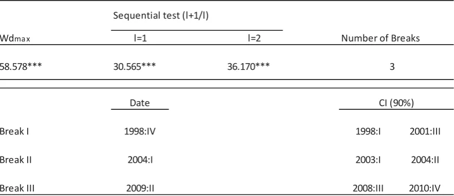
Table 2 shows the results for France. The test identifies a structural break in the behaviour
of the series that happen at the end of 1998. This is consistent with the introduction of the euro having modified the behaviour of the net external position and the adjustment
process, potentially changing the relevance of the valuation and trade components as well.
The test identifies another two breaks for France, the next one in 2004 and the last one in
2009. These two breaks seem to be more related to the real economy although the first one
is more difficult to identify. After 2004 France began to experience negative current account
and trade balances, which may have crucially affected the external adjustment process. The
last break in 2009 should be related to the global financial crisis and the recession France
suffered over that time. The global financial crisis produced important disruptions both on
the financial and the real side of the economy and it is expected that these effects could have
affected the adjustment process both for the valuation and trade components.
Table 3 presents the results for Italy. In this case the test only identifies two breaks, one in
1992 and another one in 1999. Similarly to France there is a structural break at the time of
Finally, table 5 shows the results for Germany. The test identifies two structural breaks, one
in 1989 and another one in 2006. The case for Germany is relevant as it is the only country that does not show a structural break at the time of the introduction of the euro. There could
be several reasons. First, we have to consider that Germany’s external imbalance can almost
be completely explained by the trade component, a result that will be documented in the
next section. Fuertes (2019) showed that the break in the US external position documented
at the end of fixed exchange rate regime was mainly driven by the valuation component.
It could be that Germany’s net external position was not affected by the introduction of
the euro as much as the ones from the other countries because the trade component almost
completely explains the behaviour of Germany’s external imbalance. Second, Germany is
the largest economy within the euro area and it is reasonable to think that the euro has been behaving more similarly to the Deutsche mark than any other currency and this may
have produced a less impact on the external position. Moreover, the monetary policy of the
euro zone has also been implemented to a large extent according to needs of the German
14The exchange rate mechanism established that currency fluctuations had to be contained within a margin
of 2.25% on either side of the bilateral rates (with the exception of the Italian lira, the Spanish peseta, the Portuguese escudo and the pound sterling, which were allowed to fluctuate by±6%). The United Kingdom did also abandon the exchange rate mechanism in 1992.
economy, specially before the global financial crisis, which may have reduced the impact of
the common currency. Germany’s external imbalance seems to have been more affected by
the reunification of the country in 1989 and by the global financial crisis. Both events are detected as structural breaks in the test although the one related with the global financial
crisis is stablished a little bit early at the end of 2006.
the external imbalance due to the establishment of the common currency area. The break in
1992 could be related to another event affecting the nominal exchange rate as the Italian lira
was devaluated by 7% in September of 1992 and abandoned the exchange rate mechanism
(ERM) of the European Monetary System at that time14. After this devaluation the Italian
economy experienced a large period of current account and trade surpluses.
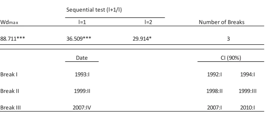
Table 4 shows the result of the structural break test for Spain. There are three structural
breaks identified: one in 1993, another one in 1999 and the last one in 2007. The test
identifies again a structural break at the time on the inception of the euro. It identifies
another break in 1993 which, similarly to the case of Italy, should be related to events
affecting the exchange rate. Even though Spain did not abandon the ERM in 1992, the
currency disruptions in the European monetary system did also affect Spain, as the Spanish government devalued the peseta by 5% in September of 1992. After that there were another
two devaluations during 1992 and 1993: a 6% devaluation in November of 1992 and a 8%
devaluation in May of 1993. This period do also coincide with a recession of the Spanish
The regression coefficients βr and βΔnx represent the share on the unconditional variance of nxa explained by the valuation component nxar and the trade component nxaΔnx. I can empirically estimate nxa, the valuation and trade components as well as the regression
coefficients βr and βΔnx using the VAR estimates. Let ˆA denote the estimated companion matrix from the VAR. The predicted value for the nxat based on our VAR estimates will be:
nxat =−(er+e
Δnx)ρAˆ(I−ρAˆ)−1Zt
=nxart +nxaΔt nx (6)
From the OLS regressions of nxart and nxaΔtnx on nxat, I can compute the variance contri-bution of the estimated valuation and trade components. From this variance decomposition
of the net external position we can obtain the relative importance of the valuation and trade
components over the external adjustment process for each of the countries under analysis.
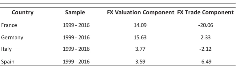
Table 6 shows this information for the period including both the years before and after the introduction of the euro. For Germany and Spain the trade component has been more
im-portant for the external adjustment. For France, the relevance of the valuation and trade
components has been almost the same and for Italy the valuation component has been
capa-ble to explain a larger share of the variance of the net external position. We have to keep in
mind that the results are not completely comparable as the sample period is not exactly the
same due to data availability. The results for Germany are striking as the trade component
almost explains all the historical variance of the external position, being the contribution of
the valuation component negligible. Moreover, the valuation component for Germany has moved in the opposite direction of the external imbalance, showing a negative covariance.
For France, Italy and Spain both the valuation and the trade components have moved in
the same direction as the external position. From these results we have to expect that if
the behaviour of Germany’s external imbalance remains similar to its historical trends, the
3.2
Valuation and Trade Effects
The results of the tests in the previous section show that the introduction of the common
currency did change the external adjustment process, at least for France, ItaIy and Spain.
Now I will use the estimates of the valuation and trade components in order to quantify
the contribution of each of them to the variance of the net external position. By doing so
with different sample periods I can assess how the external adjustment process have changed
after the introduction of the common currency. In order to find out the contribution of the
valuation and trade components to the external adjustment, I perform the following variance
decomposition:
1 =Cov(nxa, nxa)
V ar(nxa) =
Cov(nxar, nxa)
V ar(nxa) +
Cov(nxaΔnx, nxa)
V ar(nxa)
reduction of its creditor position will come from a reduction in net exports. On the other
hand, France, Italy and Spain will reduce their debtor positions by a combination of
increas-ing net exports and positive return differentials, beincreas-ing the relative important of these two
forces different for each country. As I already mentioned, Spain will restore its balanced
position mainly through increasing net exports and Italy by positive return differentials. For
France both components of external adjustment will play a similar role.
Next I analyze the changes that the introduction of the euro may have induced into the
external adjustment process. Fuertes (2019) finds for the US that the valuation component
increased its relative importance after the end of the Bretton Woods system of fixed
ex-change rate in 1973. A floating exex-change rate regime made the valuation channel to play a more prominent role on the external adjustment process. With a floating exchange rate the
valuation component not only was affected by asset price changes but also by exchange rate
changes, adding an additional source of adjustment. Under the same rationale, the valuation
component may have decreased its relative importance in the external adjustment process
of the euro area countries once the euro was in place as the bilateral external portfolio
po-sitions among the countries of the union would only change due to asset price movements.
In any case, the Bretton Woods system is not completely equivalent to the introduction
of the euro as the change for the US was from a fixed to a floating exchange rate system
while euro area countries remain with a floating exchange rates against third currencies. We
have also to take into account that there have been other events that may have affected the relative importance of the valuation and trade channels. For instance, the global financial
crisis triggered large asset price changes that may have affected the dynamics of the external
adjustment, increasing the role of valuation effects.
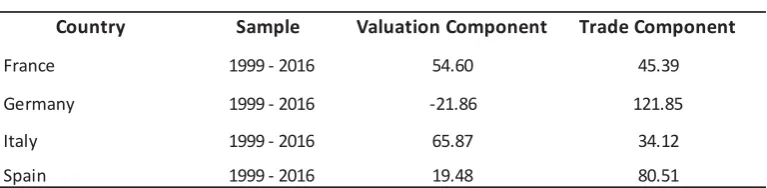
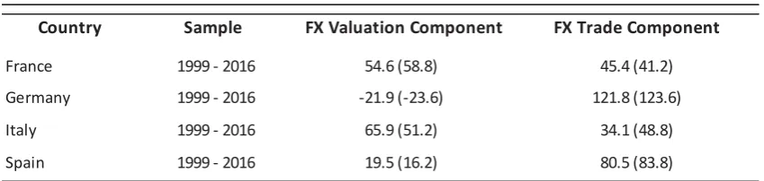
Table 7 shows the variance decomposition of the net external position between the valuation
and trade components since 1999. The results show that for Germany and Spain there is
an increase in the importance of the trade component over this period. For Spain, since the introduction of the common currency, 80% of the variance of the external imbalance is
explained by the trade component, being this number 61% if we use the whole sample. After
the introduction of the common currency Spain will have to rely more on the trade channel
in order to restore its debtor position. Similarly, for Germany the introduction of the euro
has made the country to depend even more on decreases in net exports to reduce its creditor
position. The valuation channel has increased its negative covariance with Germany’s
exter-nal imbalance during this period, making even more difficult the future exterexter-nal adjustment
of its creditor position. France and Italy on the contrary have experienced an increase in the
percentage of the variance of its external imbalance explained by the valuation component during the currency area period. This could be the result of larger asset price changes or
that exchange rate movements within the euro area countries before the introduction of the
euro were against the adjustment of the external positions of France and Italy, making the
Tables 8 and 9 present the variance of nxa explained by the exchange rate valuation compo-nent and a exchange rate trade component before and after the introduction of the euro16.
The most important conclusions from these two tables are that the exchange rates do
con-15The trade weighted exchange rates are OECD real effective exchange rates. I calculated the financial
weighted real exchange rates using the country portfolio weights that I used to calculate the portfolio returns for each of the different asset classes.
16In the case of France in table 8, due to the small sample available before 1999 I provide the results for
the whole sample instead
For Spain and Italy there has been a large decrease in the variance of nxa explained by the
exchange rate valuation component after the introduction of the euro. In the case of the exchange rate trade component , it has negatively affected the external adjustment process
after 1999 in both cases. We can then conclude that for these two countries the common cur-rency area has implied a less important role of the exchange rate in the external adjustment
and the need to rely in other mechanisms to restore the external balance. For Germany,
consistent with the tests of structural breaks that do not find any break in 1999, it seems
that there are not important changes on the contribution of the exchange rate components
between the two periods. For France, the most striking result is the large and negative
con-tribution of the exchange rate trade component during the euro period. Overall it is evident
that the reliance on the exchange rate as a tool to facilitate the external adjustment process
has largely diminished after the introduction of the euro.
17Recall that I obtain the exchange rate components by including in the VAR estimation the part of the
return differentials and net exports growth contemporaneously related with the trade weighted and financial weighted real exchange rates
Even though the results on tables 6 and 7 show that the contribution of the valuation and
trade components have indeed changed since 1999, those changes can be related to other
factors not affected by the foreign exchange regime. In order to identify, at least to some
extent, the contribution of the exchange rate regime to the external adjustment process I
have calculated a exchange rate valuation component and aexchange rate trade component.
I use a trade weighted and financial weighted real exchange rates15 to obtain the part of
the return differentials and the net exports growth that is contemporaneously related to these two real exchange rates. Then I include these exchange rate variables in the VAR
specification and compute the exchange rate trade and valuation components. These two
components will be used to compute the percentage of the variance of nxa that is explained
by the part of the valuation and trade components contemporaneously related to the real
exchange rate.
tribute to the valuation and trade components of external adjustment and also that after
1999 those contributions have changed. We should also notice that the exchange rate valu-ation component has more relevance in the external adjustment process than the exchange
rate trade component , consistent with the fact that the exchange rate may affect net exports
3.3
Future Adjustment Path
We can also make an assessment of the future adjustment paths of the external positions for
each country by computing the future expected values of nxa and the valuation and trade
components. These paths should be consistent with the relative relevance of the valuation
and trade components for each country. We can also learn how long will take to restore the
external balance for each of the economies from their current debtor or creditor positions.
We can compute the future expected adjustment path for nxa using the following equation:
ETnxaT+k =ETΔknxaT+k+nxaT
We can also compute the future adjustment path of nxa if only the valuation or the trade
components would operate:
ETnxavT+k =ETΔknxavT+k+nxaT
ETnxatT+k =ETΔknxatT+k+nxaT
Chart 4 shows the future adjustment path for Germany, being the horizontal axes the number
of quarters ahead. The red line shows the future evolution of nxa while the blue and green
lines show the evolution of nxa if only the valuation or the trade component would operate,
respectively. As we have already documented previously almost all the adjustment will be
made through the trade channel. The green line evolves very closely to the adjustment path
for nxa. Given that the valuation component hinders the restoration of Germany’s external balance, if the trade component would not play any role the external imbalance would result
in a slightly larger creditor position than the current one, as the blue line shows. If there
are not unexpected shocks affecting the future external adjustment, Germany will restore
its balanced position in 40 years. The convergence process will be much faster over the first
years, being able to reduce in half its creditor position in only 7 years.
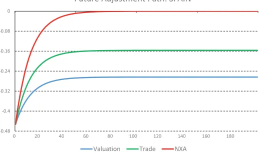
Chart 5 shows Spain’s adjustment path. We can see again how it is consistent with previous
results that showed how the trade channel is the main driver of the external adjustment.
Spain would experience a fast convergence towards an external balanced position, taking
around 19 years to reach that point. It would only take 3 years to reduce in half its debtor
position. Chart 6 presents the adjustment path for France. In this case we can see how
both the valuation and trade components almost contribute equally to the restoration of
the external balance. For France it would take a long way to achieve the external balance
although it is the country with the smallest external imbalance. It will restore its external balance in 25 years, being able to reduce it debtor position in half in 8 years. Finally chart
7 presents the future expected evolution of Italy’s external position. The contribution of the
It is reasonable to think that, as it has happened in the past, there would be unexpected
shocks that will make the expected future adjustment paths depicted in charts 4-7 differ
18The quick external adjustment expected for Italy and Spain is supported by projections from the
Inter-national Monetary Fund released in the April 2019 World Economic Outlook. These projections establish that for a group of euro are debtor countries, including Italy and Spain, the net international investment position is expected to improve by more than 25 percentages points of their collective GDP over the period 2017-2024
for different horizons k = {1,4,8}. Δket+k is the change in the real exchange rate (an increase implies an appreciation of the currency) and F Xdt is the dummy variable that from the future evolution of the external imbalances. There is relevant information we can
obtain from this exercise though. For the two countries with the largest external imbalances,
Germany and Spain, agents expect they will to be able to reduce their creditor and debtor positions by half in a relatively short period of time: 7 and 3 years respectively. The future
adjustment paths also show how all countries but Germany will need both from the valuation
and trade components to achieve their external balance. Only Germany could rely exclusively
on the trade channel, with the valuation channel playing almost no role at all.
3.4
Exchange Rate Predictability
The results from previous sections document the relationship between the net external
posi-tion and the exchange rate. It is then expected that the evoluposi-tion of the external imbalance
may have some forecasting power over the foreign exchange. This explanatory power has
already been documented by Gourinchas and Rey (2007) and Evans and Fuertes (2011),
although none of these papers study the implications of different exchange rates regimes.
On the contrary, Fuertes (2019) analyse the forecasting power of the net external position of
the U.S. over the dollar, taking into account the foreign exchange regime. The results show
that the relationship between the U.S. external imbalance and the dollar changes at the end
of the Bretton Woods system of fixed exchange rates. I will next analyse if the inception of the euro had a similar effect. I do check whether the exchange rate regime influences the
external adjustment process by regressing the changes in the real exchange rate on the net
external position, a dummy variable identifying the exchange rate regime and an interaction
term between the external position and the dummy. This interaction term will be the main
variable of interest given that a statistical significant coefficient will imply a different
rela-tion between the foreign exchange and the net external posirela-tion depending on the nominal
foreign exchange regime. I compute the OLS estimates of
1
kΔ
ke
t+k =α+β1nxat+β2F Xdt+β3nxat∗F Xdt+νt+k (7) Italy will restore the external balance in around 18 years and it will reduce it by half in less
identifies the foreign exchange regime (equals one before the introduction of the euro). I
run the regressions separately for both the real trade weighted exchange rate and the real
portfolio weighted exchange rate. For comparison purposes, I also compute the regression
without the foreign exchange regime dummy and the interaction term.
Table 10 presents the results for Spain. The coefficient β3 is significant both for the portfolio
weighted and the trade weighted real exchange rates, implying that the inception of the
euro affected the relationship between the net external position and the exchange rates. In particular, for the portfolio weighted real exchange rate, given that β1 is not significant
at any horizon in equation 7, we conclude that the forecasting power of nxa disappeared
after 1999, consistent with the decreased role played by the exchange rate in the external
adjustment process due to the common currency. As expected, the sign of the coefficients is
positive, meaning that a deterioration in the external imbalance implies a future exchange
rate depreciation. Finally, we should notice the large increase in the R2 when we run the
regression taking into account the different exchange rate regime. The R2 increases with
the exchange rate horizon, reaching a value of 0.26 when forecasting the evolution of the
exchange rate over the next two years.
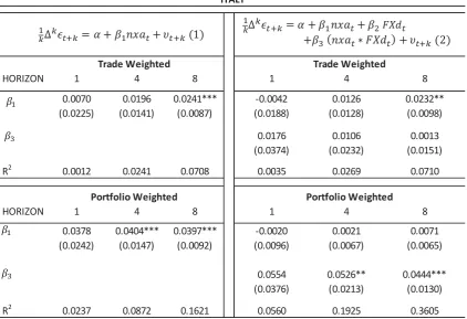
The results for Italy are presented on table 11. They are very similar to those obtained for
Spain although there is an important difference. The external imbalance has a less forecasting
power for the trade weighted real exchange rate than for the portfolio weighted one. This
could be consistent with the fact that for Italy the valuation component has more relevance
than the trade component. The R2 for the evolution of the portfolio weighted real exchange rate over the next two years reaches 0.36 in the regression that takes into account the change
in the foreign exchange regime. As it happened with Spain, the forecasting power of nxa
over the portfolio weighted exchange rate disappears after the introduction of the euro.
Table 12 shows the results for Germany. It is the country where the R2 are lower, imply-ing the weakest forecastimply-ing power of the external imbalance over the exchange rate among
the four countries. The coefficient β3 is only significant at the two year horizon and the
regression forecasting the trade weighted real exchange rate provides more significant
coef-ficients and a larger R2, consistent with the trade component having a more important role
in the external adjustment of this country. The main difference with respect to previous
results is the negative sign of the coefficient β1 in the regression that takes into account the
foreign exchange regime. The negative coefficient implies that after 1999 an improvement
of Germany’s external imbalance forecasts a depreciation of the euro. This result provides
interesting insights about the external adjustment process within a currency union. After 1999 the net external position of Italy and Spain deteriorated while Germany’s one improved.
We have documented for Italy and Spain, since 1999, that a deterioration of the external
imbalance implied a future depreciation of the trade weighted real exchange rate. During
the same period Germany improved its external imbalance, what required a future
The accuracy in estimating portfolio returns has been a topic of ample debate in the
lit-erature. In the case of the U.S. a first wave of studies calculated portfolio returns implied
from U.S. NIIP data (see Lane and Milesi-Ferretti (2005); Meissner and Taylor (2006) and
Obstfeld and Rogoff (2005)), obtaining large return differentials between portfolio assets and
liabilities. Later, Curcuru et al (2008) argued that these implied returns were upward biased due to inconsistencies in the different sources of data for flows and positions. They calculate
portfolio returns from market prices, as Gourinchas and Rey (2007) do, obtaining smaller
return differentials. Recent research from the BEA, the compilers of the NIIP data, does also
find lower estimates of portfolio return differentials than those obtained from the implied
returns in the first wave of papers, pointing out that NIIP data should not be used to obtain
returns (see Gohrband and Howell (2015)).
In this paper I computed returns from market prices in order to obtain quarterly return
differentials for a period that includes both the years before and after the introduction of the
euro. I do not claim that the implied returns may have any inconsistencies for the countries
under analysis19 as it is the case for the U.S., but I needed to construct a data set that
includes the period before the introduction of the euro. Unfortunately I could not obtain quarterly implied returns for the yeas before 1999 due to data limitations and the only option
was to estimate returns from market prices.
19Habib (2010) analyses the differential returns between gross foreign assets and liabilities for a sample of
49 countries, including France, Germany, Italy and Spain, using yearly implied returns
The results from tables 10 - 13 provide two important messages. First, the relationship
between the external imbalance and the future evolution of exchange rates is affected by
the foreign exchange regime. Second, this relationship could be different for each country within a currency union, helping or jeopardising the external adjustment process depending
on holding a debtor or a creditor position.
4
Robustness Checks
β1 may indicate that the behaviour of the euro has been driven by the needs of external
adjustment of deficit countries such as Italy and Spain, compromising the adjustment of
Germany’s external position as foreign exchange movements affect differently debtor and
creditor countries.
Finally, table 13 present the results for France. The β3 coefficients are significant and theR2
increases significantly when running the regressions taking into account the foreign exchange
rate regime. The main difference with previous results is the negative coefficientβ3, implying
that before 1999 a deterioration in France’s external imbalance forecasts an appreciation of
the french franc. After the introduction of the euro the forecasting power of nxa shows the
The equation above includes a set of restrictions on the coefficients of the VAR that repre-sent constraints on the joint dynamics of rtNF A, Δnxt, and nxat. They can be empirically examined by computing a Wald test from the estimates of theAmatrix obtained as the OLS
estimates of the VAR equations.
returns we cannot reject the null that equation (9) holds. On the contrary, the Wald test
rejects the null when using the market based returns. We should keep in mind that the mean
square errors of nxat are very low using either market based returns and derived returns. The results of the Wald test indicate that the market based returns may have incurred in
some inconsistencies that may reduce the accuracy of our estimates of the valuation and
trade component, being the implied returns more accurate to describe the joint behaviour of
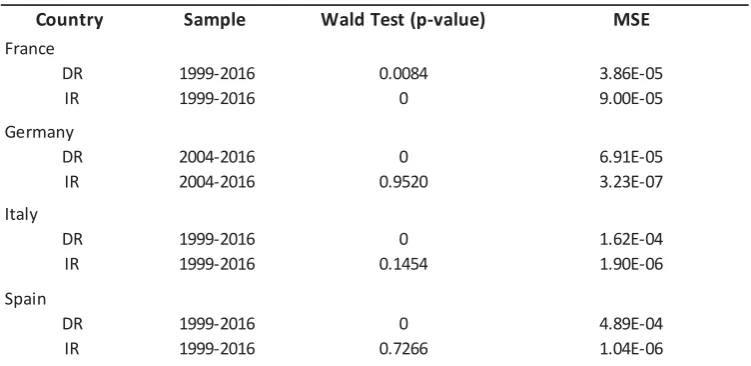
rtNF A, Δnxt, and nxat. For the case of France the Wald test rejects the null that equation (9) holds, with the MSE being larger for the predicted nxat when using the implied returns. In this case it seems that the market based returns are more accurate. We should keep in Table 14 present the results of the Wald test on the above equation as well as the mean square errors of the predicted nxat using the market based derived returns (DR) and the implied returns (IR). For Germany, Italy and Spain the Wald test shows that using the implied Then, a natural robustness check is to compute the implied returns for the years avaialble
and compare the approximation accuracy of our different estimates using the market based
returns and the implied ones. I will also assess if the main results and conclusions change
when using implied returns. In section 3.2 we already showed that the estimates of the
valuation and the trade component together are able to explain the whole variance of the
actual nxa. This is a first proof of the quality of our approximation for the present value equation (4). Another way to asses the accuracy of our approximation is to compute the
mean square error of the difference between the actual nxa and the predicted nxat, which is obtained as the sum of the estimates of the valuation and trade components. Finally, we can
also assess the accuracy of the estimates by checking if the present value equation (4) holds
using the forecasts from the VAR. In order to do we first obtain the following expression
from the present value equation (4):
enxaZt =−(er+e
Δnx) ∞
i=1
ρiAiZt
=−(er+eΔnx)ρA(I−ρA)−1Zt
(8)
This equation must hold for all possible values of Zt, such that the companion matrix A from the VAR must satisfy
mind that even though the Wald test rejects that equation (9) holds when using the market
based returns, the estimates of the valuation and trade component obtained produce very
low approximation errors and they are capable to explain the whole variance of the actual
nxa.
Because of that and despite the fact that the market based returns show some degree of
incon-sistencies for Germany, Italy and Spain, our main concern is to asses if those inconincon-sistencies
spotted out in the results of the Wald tests are large enough to invalidate the conclusions
documented in the previous sections. In particular we should be concerned about the
ca-pability of the valuation and trade components to accurately portrait the behaviour of the
net external position. Given that we have already showed that using the implied returns we obtain estimates of the valuation and trade components that provide a good approximation
of the present value equation (4), we next evaluate how different these estimates are when
using the market based return.
Table 15 shows the correlation coefficients for different series obtained using market based returns and derived returns. The first two columns show the correlation of the estimates of
the valuation and trade components obtained using the different return differentials. The
correlation coefficients are very close to one, signalling that the behaviour of the series is
almost the same no matter the returns used. The third column assess the correlation between
the predicted nxat using the two different series of return differentials, showing again that both are pretty similar. Finally, the last two column show the correlation between the
actual nxa and the predicted nxat using the implied returns and the market based returns respectively. Even though the correlations are larger for the series computed using implied
returns, except for France, the correlations are also high when using market base returns. By these metrics we can conclude that the analysis using market based returns remains valid.
Finally, I have replicated the results from table 7 using the two types of returns. Table 16 presents the percentage of the variance of nxa explained by the valuation and trade
components computed using implied returns and market based returns. The results remain
qualitatively the same no matter the series of return used. The relative relevance of the
valu-ation and trade components do not change and the percentage of variance explained is almost
the same independently of the returns used. The only country that shows some differences
is Italy although the valuation component remains as the main channel of adjustment.
Overall, even though for Germany, Italy and Spain the implied returns are more accurate to
describe the joint dynamics of rtNF A, Δnxt, and nxat embedded in the present value equa-tion (4), using the market based returns provides the same conclusions about the external
adjustment process and the estimates of the valuation and trade components are almost the
I analyze the external adjustment path of the four main economies of the euro area, covering both the period before and after the introduction of the euro, to understand if the currency
area affected their external adjustment process. I find a structural break in the net external
position for all countries but Germany at the time of the introduction of the euro, pointing
out that the inception of the common currency changed the external adjustment process.
The fact that Germany does not show this structural break is consistent with the exchange
rate regime mainly affecting the valuation channel of external adjustment, given that the
variance of Germany’s net external position is almost completely explained by the trade
channel. The importance of the valuation component of external adjustment increases after
the introduction of the euro for France and Italy, and decreases for Germany and Spain.
Third I also find that France and Italy will adjust the net external position mainly through the valuation component of external adjustment, while Germany and Spain will restore their
The results of the paper continue the debate for policy analysis on the benefits of a fixed or a
floating exchange rate regime to correct external imbalances. I document adverse valuation
effects that difficult the correction of external imbalances for the case of Germany. Even
though this should not be a matter of concern as Germany enjoys a creditor position and
reaching the external balance should not be crucial, adverse valuation affects could be
dan-gerous in other situations. For example, emerging countries with a relevant share of foreign currency liabilities and large debtor positions, could be affected by a local currency
depre-ciation as it may trigger large valuation effects that further increase their debtor positions.
The findings in this paper do also reveal the need to change the mechanisms of external
adjustment once a common currency is in place. Being the nominal exchange rate fixed
among the countries of the currency union, other adjustment mechanisms such as internal
devaluation and the change in the relative price levels. may operate. It is also important
to notice that being part of a currency union may hinder the external adjustment process
of a country as the adjustment needs are different for debtor and creditor countries. For
instance, as it is documented in this paper, the real exchange rate have evolved according to the adjusting needs of debtor countries such as Italy and Spain, pushing towards larger
external positions of creditor countries such as Germany.
5
Conclusion
external balance mostly through the trade component.
The process of external adjustment for a country within a common currency area has received little attention in the literature, despite the fact that an important mechanism of correction
of imbalances, the nominal exchange rate, has been partially cancelled. Changing from a
floating to a fixed exchange rate regime within a currency area may difficult the external
adjustment and could be potentially dangerous for countries with large negative external
positions. Understanding how the external adjustment process has evolved over time for the
countries of the euro area and the implications of the introduction of the euro are the main