Environmental Performance of Steel Grit and Specialty Sand as Abrasives

(1)

University of New Orleans University of New Orleans

ScholarWorks@UNO

University of New Orleans Theses and

Dissertations Dissertations and Theses

12-17-2004

Environmental Performance of Steel Grit and Specialty Sand as

Abrasives

Xavier Silvadasan

University of New Orleans

Follow this and additional works at: https://scholarworks.uno.edu/td

Recommended Citation Recommended Citation

Silvadasan, Xavier, "Environmental Performance of Steel Grit and Specialty Sand as Abrasives" (2004). University of New Orleans Theses and Dissertations. 200.

https://scholarworks.uno.edu/td/200

This Thesis is protected by copyright and/or related rights. It has been brought to you by ScholarWorks@UNO with permission from the rights-holder(s). You are free to use this Thesis in any way that is permitted by the copyright and related rights legislation that applies to your use. For other uses you need to obtain permission from the rights-holder(s) directly, unless additional rights are indicated by a Creative Commons license in the record and/or on the work itself.

(2)

ENVIRONMENTAL PERFORMANCE

OF

STEEL GRIT AND SPECIALTY SAND AS ABRASIVES

A Thesis

Submitted to the Graduate Faculty of the University of New Orleans

in partial fulfillment of the requirements for the degree of

Master of Science in

Civil and Environmental Engineering

by

Xavier Silvadasan

B. E. (Civil Engineering), Nagpur University, India, 1999 M. S. (Engineering Management), University of New Orleans, 2002

(3)

Acknowledgements

I would like to thank Dr. Bhaskar Kura for giving me a great opportunity to work on this

project. His experience and vast knowledge, timely help and motivation in every aspect

have been a great source of inspiration. Special thanks to my examination committee,

Dr. Kenneth McManis and Dr. Gianna Cothren for their suggestions and input in

completing this report.

I also appreciate the assistance of Mr. Byron Landry (Lab Technician, Civil Engineering)

for his active involvement in bringing up this project to the present status.

I sincerely thank Mr. Sivaramakrishnan Sangameswaran for his active participation in

the project and careful considerations in maintaining the quality of test results. Sincere

thanks are due to Ms. Sandhya Potana, Ms. Kalpalatha Kambham, Mr. Babruvahan

Hottengada and Mr. Sanjay Datar for their help in critical matters.

I would like to extend my deep appreciation towards all who helped me directly or

(4)

List of Tables

Table X-1: Abrasive Blasting Operations Summary for Test Data (AP42 ref.)

Table X-2.1: Field Data for Steel Grit

Table X-2.2: Statistical Parameters for Steel Grit

Table X-3.1: Field Data for Specialty Sand

Table X-3.2: Statistical Parameters for Specialty Sand

Table X-4.1: Minimum Emissions at Maximum Productivity

Table X-4.2: Absolute* Minimum Emissions

Table X-5: Equations for Feed Rate vs. Productivity

Table X-6: Equations for Feed Rate vs. Emission Factors (g/sqft)

Table X-7: Equations for Feed Rate vs. Emission Factors (g/lb)

Table X-8: Equations for Pressure vs. Productivity at Max. Productivity

Table X-9: Equations for Pressure vs. EF (g/sqft) at Max. Productivity

Table X-10: Equations for Pressure vs. EF (g/lb) at Max. Productivity

Table X-11: Equations for Material Feed Rate vs. Productivity

Table X-12: Equations for Material Feed Rate vs. EF (g/sqft)

Table X-13: Equations for Material Feed Rate vs. EF (g/lb)

Table X-14: Equations for Feed Rate vs. Emission Factors (g/lb) at Maximum

Productivity

Table X-15: Equations for Pressure vs. Consumption (lb/sqft)

Table X-16: Equations for Feed rate vs. EF (g/sqft) at Max. Productivity

Table X-17: Equations for Feed Rate vs. Consumption

(7)

List of Figures

Figure X-1: Steel Grit

Figure X-2: Specialty Sand

Figure X-3: Emission Test Facility at UNO.

Figure X-4: Complete Assembly of the Test Facility

Figure X-5: Schematic Diagram of Blast Pot

Figure X-6: Blast pot, blast hose with nozzle hose, respirator, air purifier, air supply hose

kit.

Figure X-7: Exhaust Duct

Figure X-8: Sampling Train

Figure X-9: Test Plate

Figure X-10: Two stage Particulate Collection System

Figure X-11: Test Plate – Before Blasting

Figure X-12: Test Plate – SP-5 SPC Finish

Figure X-15.1: Steel grit - Feed Rate vs. Productivity at 80 PSI

Figure X-15.4: Parameter Variation with Pressure at Max. Feed Rate: Steel grit

Figure X-16.1: Sand - Feed Rate vs. Productivity at 80 PSI

Figure X-16.2: Sand - Feed Rate vs. Productivity at 100 PSI

(8)

Figure X-16.4: Parameter Variation with Pressure at Maximum Feed Rate: Sand

Figure X-17: Feed Rate vs. Productivity at 80 PSI

Figure X-20: Feed Rate vs. Emission Factors (g/sqft) at 80 PSI

Figure X-23: Feed Rate vs. Emission Factors (g/lb) at 80 PSI

Figure X-26: Pressure vs. Productivity at Maximum Productivity

Figure X-27: Pressure vs. Emissions Factors (g/Sqft) at Maximum Productivity

Figure X-28: Pressure vs. Emission Factors (g/lb) at Maximum Productivity

Figure X-29: Feed Rate vs. Emission Factors (gm/lb) at Maximum Productivity

Figure X-30: Pressure vs. Consumption

Figure X-31: Feed Rate vs. Consumption at 80 PSI

Figure X-34: Feed Rate vs. Emission Factors (g/sqft) at Maximum Productivity

Figure BX-1: Graph showing minimum number of points.

Figure BX-2: Arrangement of Pitot tube and the sampling probe

Figure BX-3: Iso-kinetic Sampling

(9)

Abstract

Dry abrasive blasting is a surface preparation process used in shipyards for cleaning

the surfaces of the metal plates to be used in various components of the ship.

Commonly used abrasives include sand, steel grit, mineral abrasives, metallic

abrasives, and synthetic abrasives.

The basic objective of this study was to understand the environmental performance of

two abrasives, Steel Grit and Specialty Sand. The project was funded by the Gulf Coast

Region Maritime technology Center (GCRMTC) and USEPA. It simulated actual blasting

operations conducted at shipyards under enclosed, controlled conditions on plates

similar to steel plates commonly blasted at shipyards. The emissions were measured

using EPA Source Test Method to quantify particulate emissions.

Steel Grit was observed to be more productive, less consuming, and more

environmentally friendly compared to Specialty Sand. The findings obtained in this study

will be valuable in reducing costs, improving productivity, and protecting the

(10)

1.0 Introduction

Abrasive blasting is the use of abrasive material to clean or texturize a material such as

metal or masonry. Abrasive blasting is used in industries such as the shipbuilding

industry, automotive industry, and other industries that involve surface preparation and

painting. Dry abrasive blasting is a surface preparation process used in shipyards for

cleaning the surfaces of the metal plates to be used in various components of the ship.

The majority of shipyards no longer use sand for abrasive blasting because of concerns

about silicosis, a condition caused by respiratory exposure to crystalline silica.

Abrasive blasting presents some risks for workers' health and safety, since it has the

potential of producing air emissions. Although abrasives used in blasting booths are not

hazardous in themselves, their use can present serious danger to operators, such as

burns, falls, exposure to hazardous dusts, creation of an explosive atmosphere, and

exposure to detrimental noise. Hence it is important that both blasting booth and

blaster's equipment have to be adapted to these dangers.

The basic objective of this study was to understand the environmental performance of

two abrasives, Steel Grit and Specialty Sand. The project undertaken was a joint effort

between the Gulf Coast Region Maritime technology Center (GCRMTC) and USEPA. It

simulated actual blasting operations conducted at shipyards under enclosed, controlled

conditions on plates similar to steel plates commonly blasted at shipyards. The details

of the experimental set up and the blast equipment used are described in subsequent

(11)

using EPA Source Test Method to quantify particulate emissions. Simple mathematical

models were developed to predict performance based on feed rate and blast pressure.

1.1 Uses of Abrasive Blasting

There are numerous uses of abrasive blasting but this process usually generates a lot

of waste in the form of used abrasives and emissions. A fraction by weight of used

abrasives escapes into the atmosphere as used abrasives. The waste generated during

the abrasive blasting process is a major problem for waste management facilities due to

inconsistent waste disposal laws. Shipyards have to follow a certain track to treat the

waste generated based on its toxicity and degree of hazard. Based on the purpose and

cost estimates the most commonly used abrasives in dry blasting is usually done with

sand, metallic grit or shot, aluminum oxide (alumina), or silicon carbide.

1.2 Need for Research

Data on the productivity and emissions from the commonly used abrasives is very

limited. EPA has documented the emission factors for some of the abrasives. The first

step of their investigation was a search of the available literature relating to the

particulate emissions associated with open abrasive blasting. This search included data

contained in the open literature (e.g., National Technical Information Service); source

test reports and background documents located in the files of the EPA's Office of Air

Quality Planning and Standards (OAQPS); data base searches (e.g., SPECIATE); and

MRI's own files (Kansas City and North Carolina). The quality of the emission factors

developed from analysis of the test data was rated from A (excellent) to E (poor). The

(12)

(13)

AP-42 for abrasive blasting operations shows that the quality rating for the available

data for sand and steel grit blasting is not better than C (average). Hence, streamlined

research for generating emission factors with better data quality rating would help

shipyards choose the cleaner abrasive. Shipyards are required to obtain environmental

permits and maintain compliance that requires knowledge of the materials and

processes used. They will be able to manage the environmental matters efficiently by

knowing environmental performance of abrasives and abrasive blasting processes.

As per this discussion, it is obvious that there is a strong need for establishing

environmental performance of abrasives that would reduce shipyard costs by reducing

consumption, improve productivity, and also minimize damage to the environment and

public health.

1.3 Research Objectives

The main objective of this study was generating the dataset which would help the

shipbuilding industry in determining the right alternative that will optimize the blasting

processes. Maritime industry can use these research findings to minimize costs and

reduce the environmental factors such as pollution. Abrasive blasting is being used

widely in most shipyards. Types of abrasive materials, abrasive material gradation,

number of reuses, feed rate (lb/hr), and blast pressure (PSI) will influence the material

consumption, solid waste generation and atmospheric emissions to the ambient air.

Even the shipyard costs will be affected such as the labor costs, material costs, cleanup

(14)

Other objectives of this research are to establish relationships among process

conditions/materials and the cost/environmental parameters by measuring productivity

and waste quantities (solid/hazardous wastes and air emissions) in conjunction with the

process parameters to develop necessary mathematical relationships/models to

minimize costs and waste quantities. The specific goals of the project are to identify

relationships among process parameters/types of abrasives (independent parameters)

and environmental/cost parameters (dependent parameters) through optimization

studies. The parameters to be evaluated include:

Process parameters/Types of Abrasive:

• Abrasive feed rates (lb/hr),

• Blast pressures (PSI), and

• Gradation of abrasives.

Environmental / Cost Parameters

• Solid waste generation potential,

• Atmospheric Emissions,

• Productivity, and

(15)

2.0 Background of Study

Abrasive blasting by definition is a method of cleaning by propelling an abrasive

material through a machine and into a hose at high pressure. The main operation in

surface preparation in shipyards around the world is abrasive blasting. Abrasive blasting

can be broadly classified into three major categories:

a) Surface preparation,

b) Surface cleaning and finishing, and

c) Shot peening.

Abrasive-blasted surfaces are characterized by two kinds of information: cleanliness

and roughness. Cleanliness reflects the degree of presence of undesirable residual

contaminants on the surface. Roughness refers to the micrometric shape of the surface,

called the surface profile.

Surface preparation using blasting operations removes unwanted material and leaves a

surface ready for coating or bonding. The surface is roughened by the impact of an

angular abrasive to produce a profile. Surface cleaning and finishing differ from surface

preparation. In surface preparation, the desired result is to improve a products

appearance and usefulness rather than to condition it for coating or bonding.

To remove production contaminants and heat scale surface cleaning is used

extensively. Surface finishing includes deflashing and deburring molded parts, and

enhancing visual features. Abrasive blasting can improve the appearance of a product

by removing stains, corrosion, and tool marks. These marks are created when metal

(16)

Sometimes these processes leave residual stresses in the metal which causes those

parts to fail when stressed. By shot peening, we can increase the strength and durability

of high stress components by bombarding the surface with high velocity spherical media

namely, steel shot, ceramic shot, and glass beads.

Blasting operations basically comprise of three main elements: a propelling device, an

abrasive container, and blasting nozzle. Each component contributes towards the

overall performance of the system. The exact equipment used depends to a large extent

on the specific application and type(s) of abrasive. Air blast (or dry) systems use

compressed air to propel the abrasive using either a suction-type or pressure-type

process. The compressed air pressure system used in this project consists of a

pressure tank (pot) in which the abrasive is contained. Pressure tank is used to force

the abrasive through the blast hose rather than siphoning it. The compressed air line is

connected to both the top and bottom of the pressure tank. This allows the abrasive to

flow by gravity into the discharge hose without loss of pressure. Details of the

equipment used are described in the following chapters. The cost and properties

associated with the abrasive material dictate its application. Particulate matter (PM) and

particulate hazardous air pollutants (HAP) are the major concerns relative to abrasive

blasting. Higher wind speeds increase emissions by enhanced ventilation of the process

and by retardation of coarse particle deposition. Emissions of PM of these size fractions

are not significantly wind-speed dependent. HAPs, typically particulate metals, are

emitted from some abrasive blasting operations. These emissions are dependent on

(17)

2.1 Applications of Steel Grit

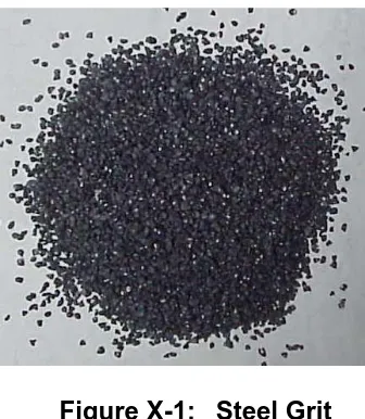
Steel Grit is commonly used today as the most powerful tool for cutting granite blocks

by gang-saws in granite industry. Steel Grit is very heavy in nature and possesses high

density as compared to other materials. The angular edges of Steel Grit are sharp and

the stability of the hardness of Steel Grit makes the cutting operation effective.

Sand-removing of large and medium sized castings, deoxidization of forgings, heat-treated

pieces, steel plates, steel pipes, sections and steel structures, intensification of springs,

surface treatment before plating, improving roughness, enhancing adhesiveness are

other applications of using Steel Grit.

Figure X-1: Steel Grit

The usefulness of Steel Grit is further glorified by the fact that it can be recycled and

reused for future experiments. On an average, the Steel Grit can be recycled over 50

(18)

2.2 Applications of Specialty Sand

Specialty Sand must meet stringent quality requirements as the principal ingredient in

the manufacture of glass, and foundry cores and molds used for metal castings. This

sand is also an ingredient in paints, refractory products and specialty fillers. It is used in

water filtration, for enhancing production of oil and gas, and in specialty construction

applications. It also satisfies recreational needs, such as golf courses, tennis courts and

ball fields. It is used in residential pool filters and sand boxes.

Figure X-2: Specialty Sand

Nearly all industries use Specialty Sand or products made with it, and for the majority of

these applications there are no known suitable substitutes. Their special properties --

purity, inertness, hardness, resistance to high temperatures, grain size and color --

(19)

3.0 Objectives

The primary objectives of this study were:

• To study the performance of Steel Grit and Specialty Sand when used in blasting

processes for enclosed conditions.

• To evaluate process parameters that can be useful for shipyards to maximize

productivity and minimize emissions.

• To estimate performance parameters related to blasting such as:

1. Productivity (defined as the area cleaned per unit time),

2. Consumption (defined as the amount of abrasive material used per unit area

cleaned),

3. Feed Rate (corresponds to the flow rate of the abrasive under given pressure

conditions), and

4. Emission Factors (defined as: (a) mass of pollutant per area cleaned, (b)

mass of pollutant per mass of abrasive used).

• To analyze the experimental results and estimate the combinations of process

(20)

4.0 Equipments Used

4.1 Test Chamber Design and Construction

Using the partial funding received through a research project funded by EPA Region 6,

an emission test facility was installed adjacent to the Engineering Building at UNO main

campus in New Orleans. The test facility measures 12 ft x 10 ft x 8 ft and was designed

as per the guidelines of EPA method 204. The chamber was constructed using plastic

sheets which were connected and riveted firmly to the wooden floor. The floor was

made up of seasoned wood and was then treated with waterproofing materials. Gaps

were sealed with silicon to prevent any seepage of the water that could interfere with

the test process. A wooden ramp was used to move the panel cart in and out of the

chamber smoothly before and after blasting. A plastic tarpaulin shed was erected

adjacent to the chamber to house the sampling equipment and test aids. More tarpaulin

(21)

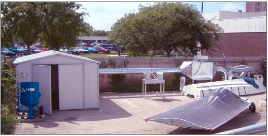
The test chamber was equipped with a fume extraction system and a two stage particle

collection system (coarse and fine particle collection). Fumes from the emission test

facility would be extracted with a variable ventilation rate, up to a maximum of 6500

cubic feet per minute (CFM) allowing capture of particles with different sizes generated

during abrasive blasting. Installed two-stage particle collection system includes an

inertial separator for coarse particles followed by bag house for fine particles. The

emissions test facility was also equipped with a 12” diameter duct to allow measurement

of particles under iso-kinetic conditions as recommended by the EPA for particle

collection from stationery sources.

Figure X-4: Complete Assembly of the Test Facility

The Blast chamber consisted of a room with internal lighting that holds both the work

piece and the operator. The operator would hold the blasting nozzle at the end of the

hose. The rusted panel rests on the wooden flooring which allowed used abrasive to

drop down for recycling. Provisions were made for proper ventilation of the blast

chamber. An exhaust window located at one end of the chamber leads to the sampling

duct through which the particulates would be collected using a variable speed fan. The

(22)

cubic feet per minute (CFM). The particles were then collected through a two-stage

particulate collection system (gravimetric and bag filters) with an efficiency of 90%, the

first stage in a drum and then through the filter bags.

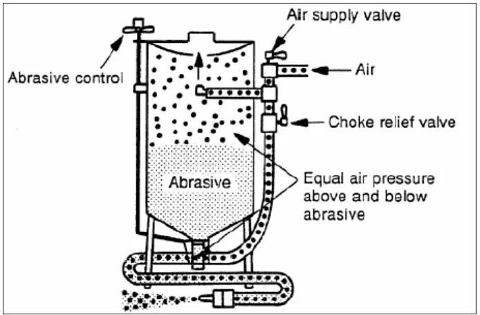
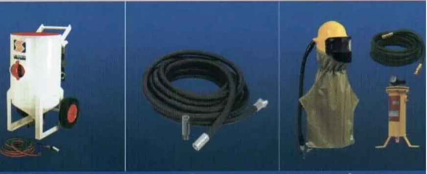
4.2 Blasting Equipment (Blast Pot)

last material using compressed air which Blast pot performs the action of propelling the b

comes from the compressor. The abrasive as well as the air will be at the same

pressure, which sweeps the abrasive towards the hose. The blast material gets mixed

with compressed air and gains its strength in the blasting equipment. The blasting

equipment known as the blast pot used in this experiment is of 600 lbs capacity and has

a 1.25 inches piping and comes with a moisture separator, air filter, and a helmet with

an air conditioning unit.

Figure X-5: Schematic Diagram of Blast Pot

(23)

Figure X-6: Blast pot; Blast hose with nozzle holder; Respirator, air purifier and

air supply hose kit.

Any lumps, dust, or other foreign material present in the material obstructs the flow by

choking the valves and interrupts the smooth flow of material. Hence proper care was

taken to make sure that there was no dust or foreign matter present in the abrasive

materials. All of the hose joints were fastened properly with the help of fasteners and

checked before each run. After the desired amount of blast material is poured into the

pot, the opening and side walls of the hopper had to be cleaned thoroughly. After

cleaning, the side opening, a small window on the side of the blast pot, as shown in Fig.

5 had to be closed tightly.

4.3 Compressor

Apart from the abrasive used, compressed air is also considered an important

component of the entire abrasive blast system. The compressor provides the air

pressure to the blasting material. A hose is used to connect the blast pot and

compressor. In the blast pot, the compressed air becomes mixed with the blasting

(24)

imparts its velocity to the blast material. The desired effect depends on many

parameters such as grain size and shape of the abrasive, pressure of the compressed

air but the velocity at which the blasting material strikes the target to be prepared is the

focal factor. The compressor used for the study was the model SULLAIR 375H, which

has a capability of providing a maximum pressure of 150 PSI. The pressures used for

the study were 80 PSI, 100 PSI and 120 PSI. The compressor is diesel operated and

wheel based with a swing down cooler, circuit breaker, two-stage air filters, and a

high/low pressure selector.

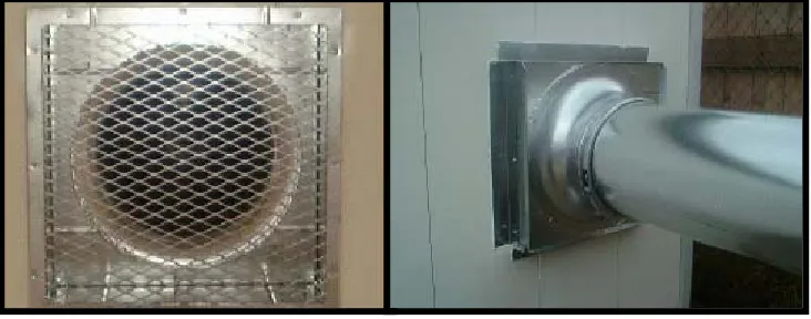
4.4 Exhaust Duct

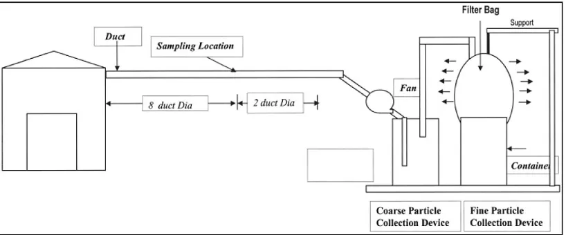
EPA method 1 for stack monitoring and testing was used to design the exhaust duct. The

diameter of the stack is 12 inches. A sampling port was located at a distance of 8 diameters

from the exhaust window and the variable speed fan was positioned at 2 diameters from

the port to minimize the turbulence on the downstream end. The exhaust window is

directly connected to the duct, which carries the emissions collected through the

exhaust. The inner portion of the duct should be smooth, straight and free of

undulations. A nozzle size of 0.18 inches turned out to be best for the test set up, which

gave fairly balanced results. (Pilot tests were conducted to determine the size of the

(25)

Figure X-7: Exhaust Duct

A standard S-type pitot tube was used for velocity measurements. It was used at a

number of positions in a cross-sectional plane perpendicular to the flow direction in the

duct to fully depict the flow. According to EPA method 1, a minimum number of

locations needed to make measurements depend on the extent of disturbance or

turbulence in the flow. A total of eight traverse points were chosen for testing for the

circular duct. The traverse points were measured and marked on the sampling probe to

ensure accuracy and ease of traverse. Iso-kinetic sampling was ensured throughout

each and every test run. Iso-kinetic samplings help in getting the representative sample

from the duct and in getting accurate test results. Getting Iso-kinetic sampling is one of

the important steps in obtaining accurate results. For ensuring iso-kinetic flow conditions

a nozzle of size of 0.18 inches was chosen for the runs. A change in the diameter of

stack or change in the direction of flow is considered as turbulence or disturbance to the

flow. The exhaust should be properly protected with mesh of proper size to remove the

(26)

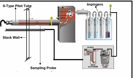
4.5 Stack Sampling Equipment

Stack sampling equipment was designed according to EPA standards and is governed

by the EPA stack sampling method 4. Stack sampling equipment has to be connected

to the sampling train and the whole arrangement can be used to collect the particulate

emission during the sampling time. The dry gas meter and thermometers mounted on

stack sampling equipment help in measuring the key parameters required for the

emission calculation.

Figure X-8: Sampling Train

For accurate measurement of the water vapor in the condenser/absorber section of the

apparatus, the probe and sample lines upstream of this section must be inert and

heated to avoid condensation, and the whole system must be free of leaks. The

apparatus consists of four glass impingers connected in series and installed in an ice

bath. The first two impingers are filled with an accurately measured quantity (100 ml) of

Impingers S-Type Pitot Tube

Stack Wall

(27)

distilled water and act as bubblers; the gas is drawn down through the cold water and

bubbles up, then travels out to the next impinger. The third impinger is left dry for further

condensation. The fourth impinger contains a quantity of silica gel (adsorbent) that

removes nearly all the remaining water vapor when the gas passes through it before

finally exiting.

4.6 Sampling Train Parts

The sampling train consists of the following parts: nozzle, the sampling probe, the filter

holder, connectors, and the impinger. In this part of the set up, the moisture gets

separated from the sample gas volume.

1. Probe and Nozzle: The probe and nozzle should be of aluminum with a sharp

tapered leading edge. The angle of taper should be on the outside to preserve a

constant internal diameter. The probe and nozzle shall be constructed of seamless

tubing.

2. Filter Holder: The filter holder is of aluminum with a screen and silicone rubber

gaskets. The holder is attached directly to the outlet of the probe. The probe and

filter holder must be constructed to be leak free.

3. Connectors: The glass connectors are used to connect the impingers with each

other and to assure air tight sealing clamps are used. Each joint is clamped properly

and securely to provide air tightness throughout the test run.

4. Impingers: There are a total of four impingers in the sampling train. The first two

impingers are filled with an accurately measured quantity of water and act as

bubblers; the impingers are known as Greenburg-Smith or modified impingers based

(28)

impinger contains a quantity of silica gel adsorbent. It helps in determining the

moisture content in the extracted sample.

4.7 Plate Size Specifications

The test panels used in these blasting operations were made of cast iron of area 40 sqft. (8’x5’).

The experiments were conducted for surfaces with flash rust. A total of four plates were used and

they were mounted on a panel cart. The results presented in this document correspond to blasting

of plates having flash rust generated by the action of moisture and air on the exposed plates.

Typically the plates were allowed to rust after every blasting run for around 24 hours (average

over all the runs) to ensure uniform rust.

Figure X-9: Test Plate

To support the plates during the experiment a panel cart was used. The panel cart was

chosen in such a way that two plates can be mounted at a time and can be turned using

the castors during the experiment if needed.

4.8 Schmidt Valve

Feed rate of the abrasive used was governed by the number of turns of Schmidt valve when it is

(29)

minimum of one turn to a maximum of nine and half turns. In this study, the turns used

were 3, 4, and 5 turns of the open Schmidt valve to specify the feed rate used.

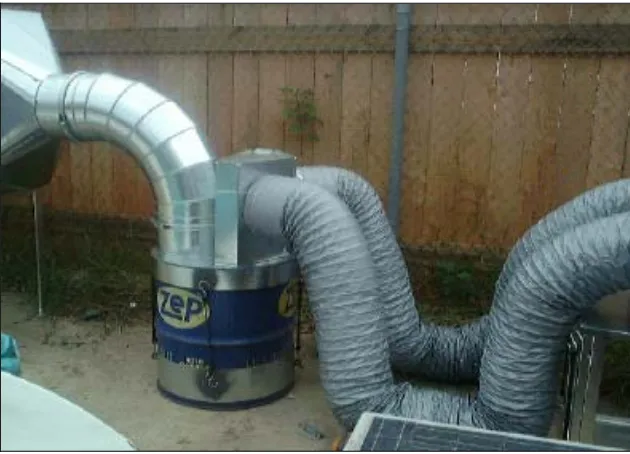
4.9 Particulate Collection System

For collecting the particles emitted during the blasting experiments, a two-stage particle

collection system (Refer to Figure 13) is installed at test facility which includes an

inertial separator for coarse particles followed by bag house for fine particles. The

emission test facility is equipped with a long 12” diameter duct to allow measurement of

particles under iso-kinetic conditions as recommended by the EPA for particle collection

from stationery sources. The two stage particulate collection system is designed to trap

the maximum amount of emissions and to prevent it from becoming airborne. In the first

stage the exhaust duct is diverted into a 55-gallon drum after passing the sampling

train. In this process the coarser particles settle down at the bottom of the drum and

thus will be removed from the system.

(30)

The second stage of the collection system is used for the finer particles. In the second

stage of the collection system, the particles from the outlet of the 55-gallon drum are

diverted towards the inlet of the filter bags. In this stage, the coarser particles escaped

from the first stage with the finer particles becoming trapped in the side wall of the

filters. In the study, four filter panels were used. Each filter panel consisted of five

individual filters that help in trapping more and more emissions and preventing them

from becoming airborne, thus increasing the efficiency of the overall collection system.

4.10 Test Constraints

Number of different factors rule the particulate emissions such as, (1) blast pressure, (2)

feed rate, (3) blast nozzle size, (4) grade of abrasive used, (5) exhaust rate, (6) exhaust

flow pattern, (7) orientation of the plate inside the test chamber, (8) distance between

the plate and the blast nozzle, (9) angle of the blast nozzle with respect to the test plate,

(10) surface finish required, and (11) surface contamination at the beginning. Though

every effort was made to simulate field conditions, it is important to note the conditions

of this study.

• Blast pressure and feed rates were measured for all runs in the study and the

results are expressed with respect to these parameters.

• Blast nozzle used was size # 6 (Bozzuka) for all test runs.

• Medium grade Steel Grit and 20-40 grade Specialty Sand were used without

a recycling option.

• Exhaust rate of 3200 cfm (average) was used.

(31)

• An average distance of 12” was maintained between the test plate and the

blast nozzle.

• Blast nozzle was kept perpendicular to the plate as much as possible.

• Surface finish quality maintained was near to commercial finish (SPC-6).

• Flash rusting was used as the surface contamination for all test plates.

(32)

5.0 Field Test Procedure

Field testing at UNO Emissions test facility included two major steps:

1. Perform the blasting of test panels using Steel Grit and Specialty Sand, and

2. Stack/Source sampling for evaluation of particulate emissions.

Blasting was performed by following the commonly observed shipyard blasting

procedures including Society of Protective Coating (SPC) recommendations. SPC has

visual standards (section 5.2) to characterize the metal surface that is cleaned using

abrasives. For source sampling, EPA’s emissions test methods 1 through 5 were used

which are discussed in Appendix B.

First, the rusted test panels were mounted on the cart with one on either side. A

measured amount of abrasive was transferred into the blast pot through a sieve to

remove any foreign material that may interfere with the smooth flow of the abrasive. The

compressor was used to supply compressed air to the blast pot. Stack sampling

equipment was used for the sample collection at various traverse points which were

marked on the probe in advance. The sampling train was connected properly with

impingers in position and leak tests were done to make sure the connections were tight.

The Schmidt valve was adjusted for the desired number of turns, the compressor was

turned on, the blasting pressure was adjusted to the desired setting (80, 100, 120 PSI at

the nozzle), and then the blasting was initiated.

The sampling probe was inserted into the sampling port and the necessary parameters,

namely, velocity head, stack temperature, vacuum, DGM readings, and box

(33)

traverse points. After the blasting and source sampling, the filters used in the test along

with sampling probe were taken to the laboratory for analysis.

The filter was weighed and the sampling probe was rinsed thoroughly with acetone to

get the remaining particulates stuck on the side of the wall in a pre-weighed beaker. The

difference between the final weight of the filter and the initial weight of the filter plus the

final weight and initial weight of the beaker after evaporating the acetone and acetone

blank test gives the particulate loading for the volume of gas sampled. After this step,

the leak test was performed again to check for leakage in the sampling train.

Below sequence was used to perform various field activities:

• Obtain the values for barometric pressure and temperature.

• Calculate K factor necessary for iso-kinetic sampling. (∆H = K x ∆P) using

these values and the nozzle diameter. Set up the instrument and sampling

train on site.

• Perform leak check on sampling train before the actual tests.

• Note down various parameters needed for the run such as velocity head,

stack temperature, vacuum, DGM readings, box temperature, etc.

• Perform leak check on sampling train after the actual tests.

• Obtain the percentage isokinetic from the observed parameters and formulae

listed in the EPA methods (within 90% to 110%).

• Get the particulate loading by weighing the filters and beaker, in the

(34)

5.1 Input and Output Variables

Dry abrasive blasting results are influenced by primary parameters such as initial

surface conditions, final surface conditions desired, abrasive type, abrasive grade, blast

pressure, feed rate, surface conditions, angle of abrasive jet, blast nozzle size, distance

from nozzle to the surface, worker training, worker awareness on environmental issues,

worker weariness, ventilation conditions, fan capacity in case of blast houses, and wind

speed in case of open-air conditions.

Blasting and source sampling was carried out in a trained way to minimize the human

errors by maintaining the conditions uniform and ensuring that site parameters and

blasting conditions are consistent across different runs.

The parameters that formed input variable set are defined as follows:

1. Abrasive: The abrasives tested were Steel Grit and Specialty Sand.

2. Blast Pressure: The tests were conducted at 3 blast pressures which were 80

PSI, 100 PSI, and 120 PSI.

3. Feed rate: Feed rate of the abrasive was varied using Schmidt valve connected

to the bottom of the blast pot. The number of turns used was 3, 4 and 5 turns in

open condition of the valve.

4. Nozzle Size: A nozzle of diameter 0.18 inches was chosen to ensure iso-kinetic

sampling conditions.

5. Blasting Time: The total blasting time was measured for each run using a stop

watch. The sampling time was constant for all the runs: 2 minutes at each

(35)

The parameters measured in the field specific to each run form the output parameter set

and are defined as follows:

1. Area Cleaned: The blasted area was calculated using a measuring tape.

Necessary corrections were made for accurately measuring the area cleaned.

2. Productivity: Productivity is a measure of blasting speed and is defined as

Productivity (sqft/hr) = Area Cleaned (sqft) / Total Blasting Time (hours)

3. Emission Factors: The emission factors are expressed in this report in terms of

the following units:

a. Mass of pollutant emitted (g) / Area Cleaned (sqft)

b. Mass of Pollutant emitted (g) / Quantity of abrasive used (lb)

c. Mass of Pollutant emitted (lb) / Quantity of abrasive used (lb)

d. Mass of Pollutant emitted (lb) / Quantity of abrasive used (ton)

4. Consumption: It is defined as

Consumption = Quantity of Abrasive Used (lb) / Area Cleaned (sqft)

5. 2 Surface Preparation Standards

The SPC developed visual standards for the finished surface using a range between

SP-1 to SP-11. In this study, the finish of test panels varied between SP-5, SP-6, and

SP-10 grades. The finish depended on the blast pressure and the feed rate of abrasive.

The surface characteristics of rusted panels and blasted panels are illustrated in the

(36)

Figure X-11: Test Plate - Before Blasting

5.2.1 SP-5 SPC Standard (White Metal Blasting)

This standard is defined as the removal of all visible rust, mill scale, paint and

contaminants which leaves the metal uniformly white or gray in appearance. It is the

ultimate in blast cleaning.

Figure X-12: Test Plate - SP-5 SPC Finish

5.2.2 SP-6 SPC Standard (Commercial Blast)

Foreign matter like oil, grease, dirt, and rust scale are completely removed from the

surface and all rust, mill scale, and old paint are completely removed by abrasive

blasting except for slight shadows, streaks or discolorations caused by rust stain, mill

scale oxides, or slight, tight resides of paint or coating that remain. If the surface is

(37)

two-thirds of each square inch of the surface area shall be free of all visible residues and

the remainder shall be limited to the light residues mentioned above.

Figure X-13: Test Plate - SP-6 SPC Finish

5.2.3 SP-10 SPC Standard (Brush-off Blast)

Except for very light shadows, very slight streaks or slight discolorations caused by rust

stain, mill scale oxides, or slight, tight residues of paint or coating all other foreign

matter such as oil, grease, dirt, mill scale, rust, corrosion products, oxides, and paint,

are completely removed from the surface by abrasive blasting. At least 95% of each

square inch of surface area shall be free of all visible residues, and the remainder shall

be limited to the light discolorations mentioned above. From a practical standpoint, this

is probably the best quality surface preparation that can be expected today for existing

plant facility maintenance work.

(38)

6.0 Results

Field results of the blasting project are listed in this section. Table X-2.1 gives the field

data observed for Steel Grit and Table X-2.2 shows the statistical parameters (mean

and standard deviations) of productivity (sqft/hr), consumption (lb/sqft) and emission

factors (g/sqft, g/lb, and lb/ton) for Steel Grit. Tables X-3.1 and X-3.2 show

corresponding data for Specialty Sand. The columns in these tables can be read as

follows:

Column 1: Pressure: Pressure (Pounds per Square Inch).

Column 2: No. of Turns: Number of turns of the open Schmidt valve.

Column 3: Weight (or Wt): Weight of the abrasive used (pounds).

Column 4: B Time: Blasting time (minutes).

Column 5: MCR: Material Consumption Rate (pounds per minute).

Column 6: A: Cleaned area of the plate (square feet).

Column 7: E: Quantity of emissions obtained in the sampling train (grams of pollutant

mass collected).

Column 8: P: Productivity (square feet per hour).

Column 9: C: Consumption (pounds per square feet).

Column 10: Emission Factors: Emission factor represented as:

• Mass of pollutant per area cleaned (grams per square feet).

• Mass of pollutant per amount of abrasive consumed. (gm/lb, lb/lb, lb/kg, lb/ton).

(39)

Table X-4.1 shows the Steel Grit and Specialty Sand producing minimum emissions

with respect to maximum productivity at a corresponding pressure and number of turns.

Table X-4.2 summarizes the absolute minimum emissions (gm/sqft) without considering

productivity for the two abrasives at the three pressures. These two tables would be

helpful to shipyards for choosing the cleaner abrasive among these two based on their

needs. For steel grit at 120 PSI, the valve opening was not a constraint. Also, the

material consumption rate was constant and the blasting time solely depended on

pressure.

Figures X-15.1, X-15.2, X-15.3 show the productivity variation at pressures 80 PSI, 100

PSI, and 120 PSI respectively for Steel Grit and Figure X-15.4 shows the parameter

variation with pressure at maximum feed rate for Steel Grit. A similar numbering

(40)

Press Turns Wt BT MCR A E P C EF1 EF2

PSI lbs min lbs/min sqft g sqft/hr lb/sqft g/sqft g/lb lb/lb lb/ton

120 3 50 6 8.33 20 223.58 200.00 2.500 11.179 4.472 0.0099 19.72

120 3 50 6 8.33 22 217.47 220.00 2.273 9.885 4.349 0.0096 19.18

120 3 50 6 8.33 18 202.85 180.00 2.778 11.269 4.057 0.0089 17.89

120 4 50 6 8.33 26 221.26 260.00 1.923 8.510 4.425 0.0098 19.52

120 4 50 6 8.33 28 203.61 280.00 1.786 7.272 4.072 0.0090 17.96

120 4 50 6 8.33 27 199.67 270.00 1.852 7.395 3.993 0.0088 17.61

120 5 50 6 8.33 25 247.84 250.00 2.000 9.914 4.957 0.0109 21.86

120 5 50 6 8.33 24 227.51 240.00 2.083 9.480 4.550 0.0100 20.07

120 5 50 6 8.33 26 237.65 260.00 1.923 9.140 4.753 0.0105 20.96

100 3 50 5 10.00 22 163.04 264.00 2.273 7.411 3.261 0.0072 14.38

100 3 50 5 10.00 21 171.11 252.00 2.381 8.148 3.422 0.0075 15.09

100 3 50 6 8.33 20 157.74 200.00 2.500 7.887 3.155 0.0070 13.91

100 4 50 10 5.00 22 187.78 132.00 2.273 8.535 3.756 0.0083 16.56

100 4 50 11 4.55 24 190.76 130.91 2.083 7.948 3.815 0.0084 16.83

100 4 50 10 5.00 24 176.77 144.00 2.083 7.365 3.535 0.0078 15.59

100 5 50 4 12.50 18 194.63 270.00 2.778 10.813 3.893 0.0086 17.17

100 5 50 5 10.00 22 193.30 264.00 2.273 8.786 3.866 0.0085 17.05

100 5 50 5 10.00 19 198.13 228.00 2.632 10.428 3.963 0.0087 17.48

80 3 50 6 8.33 18 148.77 180.00 2.778 8.265 2.975 0.0066 13.12

80 3 50 6 8.33 18 139.12 180.00 2.778 7.729 2.782 0.0061 12.27

80 3 50 6.5 7.69 19 167.64 175.38 2.632 8.823 3.353 0.0074 14.79

80 4 50 6 8.33 20 168.29 200.00 2.500 8.415 3.366 0.0074 14.84

80 4 50 6 8.33 19.5 187.17 195.00 2.564 9.598 3.743 0.0083 16.51

80 4 50 6 8.33 19 170.81 190.00 2.632 8.990 3.416 0.0075 15.07

80 5 50 9 5.56 27 191.16 180.00 1.852 7.080 3.823 0.0084 16.86

80 5 50 9 5.56 30 200.98 200.00 1.667 6.699 4.020 0.0089 17.73

80 5 50 9 5.56 28 186.02 186.67 1.786 6.644 3.720 0.0082 16.41

(41)

Press Turns Wt P C Emission Factors

PSI lbs sqft / hr Mean SD lb/sqft Mean SD g/sqft Mean SD g/lb Mean SD lb/ton Mean SD

120 3 50 200.00 2.500 11.179 4.472 19.72

120 3 50 220.00 200.00 20.00 2.273 2.52 0.25 9.885 10.78 0.77 4.349 4.29 0.21 19.18 18.93 0.94

120 3 50 180.00 2.778 11.269 4.057 17.89

120 4 50 260.00 1.923 8.510 4.425 19.52 120 4 50 280.00 270.00 10.00 1.786 1.85 0.07 7.272 7.73 0.68 4.072 4.16 0.23 17.96 18.36 1.01 120 4 50 270.00 1.852 7.395 3.993 17.61

120 5 50 250.00 2.000 9.914 4.957 21.86

120 5 50 240.00 250.00 10.00 2.083 2.00 0.08 9.480 9.51 0.39 4.550 4.75 0.20 20.07 20.96 0.90

120 5 50 260.00 1.923 9.140 4.753 20.96

100 3 50 264.00 2.273 7.411 3.261 14.38

100 3 50 252.00 238.67 34.02 2.381 2.38 0.11 8.148 7.82 0.37 3.422 3.28 0.13 15.09 14.46 0.59

100 3 50 200.00 2.500 7.887 3.155 13.91

100 4 50 132.00 2.273 8.535 3.756 16.56

100 4 50 130.91 135.64 7.26 2.083 2.15 0.11 7.948 7.95 0.59 3.815 3.70 0.15 16.83 16.33 0.65

100 4 50 144.00 2.083 7.365 3.535 15.59

100 5 50 270.00 2.778 10.813 3.893 17.17 100 5 50 264.00 254.00 22.72 2.273 2.56 0.26 8.786 10.01 1.08 3.866 3.91 0.05 17.05 17.23 0.22 100 5 50 228.00 2.632 10.428 3.963 17.48

80 3 50 180.00 2.778 8.265 2.975 13.12

80 3 50 180.00 178.46 2.66 2.778 2.73 0.08 7.729 8.27 0.55 2.782 3.04 0.29 12.27 13.39 1.28

80 3 50 175.38 2.632 8.823 3.353 14.79

80 4 50 200.00 2.500 8.415 3.366 14.84 80 4 50 195.00 195.00 5.00 2.564 2.57 0.07 9.598 9.00 0.59 3.743 3.51 0.21 16.51 15.47 0.90 80 4 50 190.00 2.632 8.990 3.416 15.07

80 5 50 180.00 1.852 7.080 3.823 16.86

80 5 50 200.00 188.89 10.18 1.667 1.77 0.09 6.699 6.81 0.24 4.020 3.85 0.15 17.73 17.00 0.67

80 5 50 186.67 1.786 6.644 3.720 16.41

(42)

Press Turns Wt BT MCR A E P C EF1 EF2

PSI lbs min lbs/min sqft g sqft/hr lb/sqft g/sqft g/lb lb/lb lb/ton

120 3 100 10 10.00 31 1078.89 186.00 3.226 34.803 10.789 0.0238 47.58

120 3 100 11 9.09 33 992.84 180.00 3.030 30.086 9.928 0.0219 43.78

120 3 100 8 12.50 25 971.01 187.50 4.000 38.840 9.710 0.0214 42.82

120 4 100 9 11.11 34.5 1070.36 230.00 2.899 31.025 10.704 0.0236 47.20

120 4 100 9 11.11 33.5 1053.06 223.33 2.985 31.435 10.531 0.0232 46.44

120 4 100 9 11.11 33 995.01 220.00 3.030 30.152 9.950 0.0219 43.88

120 5 100 8 12.50 25 1217.95 187.50 4.000 48.718 12.180 0.0269 53.71

120 5 100 11 9.09 33.5 1180.27 182.73 2.985 35.232 11.803 0.0260 52.05

120 5 100 10 10.00 31 1240.77 186.00 3.226 40.025 12.408 0.0274 54.72

100 3 100 12 8.33 24 1044.56 120.00 4.167 43.523 10.446 0.0230 46.07

100 3 100 10 10.00 21 1050.01 126.00 4.762 50.000 10.500 0.0232 46.31

100 3 100 11.5 8.70 24 1096.01 125.22 4.167 45.667 10.960 0.0242 48.33

100 4 100 13 7.69 32 1108.09 147.69 3.125 34.628 11.081 0.0244 48.87

100 4 100 12.5 8.00 29 1088.32 139.20 3.448 37.528 10.883 0.0240 47.99

100 4 100 10.5 9.52 26 1111.58 148.57 3.846 42.753 11.116 0.0245 49.02

100 5 100 12 8.33 27 1141.07 135.00 3.704 42.262 11.411 0.0252 50.32

100 5 100 12.5 8.00 28 1127.92 134.40 3.571 40.283 11.279 0.0249 49.74

100 5 100 11.5 8.70 26 1118.85 135.65 3.846 43.033 11.189 0.0247 49.34

80 3 100 15 6.67 32 954.96 128.00 3.125 29.843 9.550 0.0211 42.11

80 3 100 13 7.69 27.5 962.15 126.92 3.636 34.987 9.622 0.0212 42.43

80 3 100 13.5 7.41 27 977.67 120.00 3.704 36.210 9.777 0.0216 43.12

80 4 100 14.5 6.90 31 925.20 128.28 3.226 29.845 9.252 0.0204 40.80

80 4 100 13.5 7.41 29 1025.20 128.89 3.448 35.352 10.252 0.0226 45.21

80 4 100 14 7.14 30 940.98 128.57 3.333 31.366 9.410 0.0207 41.50

80 5 100 13.5 7.41 30 996.80 133.33 3.333 33.227 9.968 0.0220 43.96

80 5 100 12 8.33 26.5 1008.68 132.50 3.774 38.063 10.087 0.0222 44.48

80 5 100 11.5 8.70 26.5 1029.19 138.26 3.774 38.837 10.292 0.0227 45.39

(43)

Press Turns Wt P C Emission Factors

PSI lbs sqft / hr Mean SD lb/sqft Mean SD g/sqft Mean SD g/lb Mean SD lb/ton Mean SD

120 3 100 186.00 3.226 34.803 10.789 47.58

120 3 100 180.00 184.50 3.97 3.030 3.42 0.51 30.086 34.58 4.38 9.928 10.14 0.57 43.78 44.73 2.52

120 3 100 187.50 4.000 38.840 9.710 42.82

120 4 100 230.00 2.899 31.025 10.704 47.20 120 4 100 223.33 224.44 5.09 2.985 2.97 0.07 31.435 30.87 0.66 10.531 10.39 0.39 46.44 45.84 1.74 120 4 100 220.00 3.030 30.152 9.950 43.88

120 5 100 187.50 4.000 48.718 12.180 53.71

120 5 100 182.73 185.41 2.44 2.985 3.40 0.53 35.232 41.32 6.84 11.803 12.13 0.31 52.05 53.49 1.35

120 5 100 186.00 3.226 40.025 12.408 54.72

100 3 100 120.00 4.167 43.523 10.446 46.07

100 3 100 126.00 123.74 3.26 4.762 4.37 0.34 50.000 46.40 3.30 10.500 10.64 0.28 46.31 46.90 1.25

100 3 100 125.22 4.167 45.667 10.960 48.33

100 4 100 147.69 3.125 34.628 11.081 48.87 100 4 100 139.20 145.15 5.18 3.448 3.47 0.36 37.528 38.30 4.12 10.883 11.03 0.13 47.99 48.63 0.55 100 4 100 148.57 3.846 42.753 11.116 49.02

100 5 100 135.00 3.704 42.262 11.411 50.32

100 5 100 134.40 135.02 0.63 3.571 3.71 0.14 40.283 41.86 1.42 11.279 11.29 0.11 49.74 49.80 0.49

100 5 100 135.65 3.846 43.033 11.189 49.34

80 3 100 128.00 3.125 29.843 9.550 42.11

80 3 100 126.92 124.97 4.34 3.636 3.49 0.32 34.987 33.68 3.38 9.622 9.65 0.12 42.43 42.55 0.51

80 3 100 120.00 3.704 36.210 9.777 43.12

80 4 100 128.28 3.226 29.845 9.252 40.80

80 4 100 128.89 128.58 0.31 3.448 3.34 0.11 35.352 32.19 2.84 10.252 9.64 0.54 45.21 42.50 2.37

80 4 100 128.57 3.333 31.366 9.410 41.50

80 5 100 133.33 3.333 33.227 9.968 43.96 80 5 100 132.50 134.70 3.11 3.774 3.63 0.25 38.063 36.71 3.04 10.087 10.12 0.16 44.48 44.61 0.72 80 5 100 138.26 3.774 38.837 10.292 45.39

(44)

S No Pressure Feed rate

Maximum

Productivity Emission Factors (PSI) (No. of turns) (sqft/hr) g/sqft g/lb lb/ton

Steel grit 80 4 195 9.00 3.51 15.47

100 5 254 10.01 3.91 17.23

120 4 270 7.73 4.16 18.36

Specialty

Sand 80 5 134.7 36.71 10.12 44.61

100 4 145.15 38.30 11.03 48.63

120 4 224.44 30.87 10.39 45.84

Table X-4.1: Minimum Emissions at Maximum Productivity (gm/sqft)

From the above table, it is imperative that Steel Grit is giving higher productivity among

the two abrasives compared. This implies that more area can be cleaned in a lesser

time frame. It is also worth noting that Specialty Sand is giving out higher emissions

when compared to Steel Grit. This implies that the mass of pollutant emitted is higher

for a specific mass of Specialty Sand used. Steel Grit emits less pollutant per square

feet of cleaned area.

S No Pressure Feed rate Emission Factors (PSI) (No. of turns) g/sqft g/lb lb/ton

Steel grit 80 5 6.81 3.85 17.00

100 3 7.82 3.28 14.46

120 4 7.73 4.16 18.36

Specialty

Sand 80 4 32.19 9.64 42.50

100 4 38.30 11.03 48.63

120 4 30.87 10.39 45.84

Table X-4.2: Absolute* Minimum Emissions (without considering Productivity)

According to the above table, emission factors with respect to area cleaned for Steel

Grit increases with increase in pressure but this trend is not clear for emission factors

with respect to abrasive quantity. For Steel Grit, low pressure-high feed rate

combination corresponds to the lowest emissions whereas for Specialty Sand, feed rate

(45)

Figure X-15.1: Steel grit - Feed Rate vs Productivity at 80 PSI

y = -11.325x2 + 95.812x - 7.0513 R2_{= 0.6071}

175.00 180.00 185.00 190.00 195.00 200.00 205.00

2 3 4 5

Feed Rate (No. of Turns)

P ro d uc ti v it y (s qft /hr ) 6

y = 110.7x2 - 877.91x + 1876.1 R2_{= 0.8781}

125.00 145.00 165.00 185.00 205.00 225.00 245.00 265.00 285.00

2 3 4 5

(46)

y = -45x2_{+ 385x - 550}

R2 = 0.8667

175.00 195.00 215.00 235.00 255.00 275.00 295.00

2 3 4 5

Figure X-15.4: Parameter Variation with Pressure at Maximum Feed Rate: Steel grit

0.00 50.00 100.00 150.00 200.00 250.00 300.00

70 80 90 100 110 120 130

(47)

Figure X-16.1: Sand: Feed Rate vs Productivity at 80 PSI

y = 1.2575x2 - 5.198x + 129.25 R2 = 0.7168

110.00 120.00 130.00 140.00 150.00

2 3 4 5

y = -15.776x2 + 131.85x - 129.82 R2 = 0.901

120.00 130.00 140.00 150.00

2 3 4 5

(48)

y = -39.49x2 + 316.37x - 409.21 R2 = 0.9704

170.00 180.00 190.00 200.00 210.00 220.00 230.00 240.00

2 3 4 5

Figure X-16.4: Parameter Variation with Pressure at Maximum Feed Rate: Sand 0.00 50.00 100.00 150.00 200.00 250.00

70 80 90 100 110 120 130

(49)

Figure X-17: Feed Rate vs Productivity at 80 PSI

Sand

y = 1.2575x2 - 5.198x + 129.25 R2 = 0.7168

Steel grit

y = -11.325x2 + 95.812x - 7.0513 R2 = 0.6071

0.00 50.00 100.00 150.00 200.00 250.00

2 3 4 5 6

P rod uc ti v ity ( s qft /hr ) Steel grit Sand

Figure X-18: Feed Rate vs Productivity at 100 PSI

Sand

y = -15.776x2 + 131.85x - 129.82 R2 = 0.901 Steel grit y = 110.7x2 - 877.91x + 1876.1

R2 = 0.8781

50.00 100.00 150.00 200.00 250.00 300.00

2 3 4 5 6

(50)

Figure X-19: Feed rate vs Productivity at 120 PSI

Steel grit

y = 4.0754x2 - 35.329x + 270.83 R2_{= 0.8037}

Sand

y = -39.49x2_{+ 316.37x - 409.21}

R2 = 0.9704

50.00 100.00 150.00 200.00 250.00 300.00

2 3 4 5 6

P rod uc ti v ity ( s qft /hr ) Steel grit Sand

Figure X-20: Feed Rate vs Emission Factors (g/sqft) at 80 PSI

Sand

y = 2.2521x2 - 16.845x + 61.105 R2 = 0.402

Steel grit

y = -1.3351x2_{+ 9.9666x - 10.339}

R2 = 0.8934 0.000 10.000 20.000 30.000 40.000 50.000 60.000

2 3 4 5 6

(51)

Sand

y = 5.472x2 - 46.3x + 132.79 R2 = 0.6954

Steel grit

y = 0.7709x2_{- 5.1314x + 15.528}

R2 = 0.7814

0.000 10.000 20.000 30.000 40.000 50.000 60.000

2 3 4 5 6

E m iss io n F act o rs (g m /sq ft ) Steel grit Sand

Sand

y = 4.5589x2_{- 33.207x + 89.668}

R2 = 0.5177

Steel Grit y = 1.719x2_{- 14.275x + 37.091}

R2 = 0.8618

0.000 10.000 20.000 30.000 40.000 50.000 60.000

2 3 4 5 6

(52)

Figure X-23: Feed Rate vs Emission Factors (g/lb) at 80 PSI

Sand

y = 0.0745x2 - 0.4422x + 9.4983 R2_{= 0.95}

Steel Grit

y = -0.0655x2 + 0.8715x + 0.7452 R2 = 0.773

0.000 2.000 4.000 6.000 8.000 10.000 12.000

2 3 4 5 6

E m is s ion Fa c tors (g/ lb ) Steel grit Sand

Figure X-24: Feed Rate vs Emission factors (g/lb) at 100 PSI

Sand

y = -0.0429x2 + 0.5373x + 8.6625 R2 = 0.7335

Steel grit

y = -0.1445x2_{+ 1.4605x - 0.1132}

R2 = 0.853

0.000 2.000 4.000 6.000 8.000 10.000 12.000

2.5 3 3.5 4 4.5 5 5.5

(53)

Figure X-25: Feed Rate vs Emission Factors (g/lb) at 120 PSI

Sand

y = 0.0607x2 + 0.4754x + 7.1514 R2_{= 0.8925}

Steel grit y = 0.0688x2 - 0.32x + 4.221

R2_{= 0.7614}

0.000 2.000 4.000 6.000 8.000 10.000 12.000

2 2.5 3 3.5 4 4.5 5 5.5

Em iss io n F act o rs ( g /lb ) Steel grit Sand

Figure X-26: Pressure vs Productivity at Maximum Productivity

Sand

y = 0.0861x2 - 14.967x + 781.3 Steel Grit y = -0.0537x2 + 12.625x - 471

0.00 50.00 100.00 150.00 200.00 250.00 300.00

70 80 90 100 110 120 130

(54)

Figure X-27: Pressure vs Emissions Factors (g/Sqft) at Maximum Productivity

Sand

y = -0.0091x2 + 1.745x - 47.86

Steel grit y = -0.0033x2 + 0.638x - 21.91 0 50 100 150 200 250

70 80 90 100 110 120 130

Pressure (PSI) Em issio n F a c to rs ( g /S q ft ) 0.00 5.00 10.00 15.00 20.00 25.00 30.00 35.00 40.00

Steel grit - sec axis Sand - sec axis

Figure X-28: Pressure vs Emission Factors (g/lb) at Maximum Productivity

Steel grit y = 8E-05x2 + 0.0065x + 2.18

Sand

y = -0.0013x2 + 0.2892x - 5.43

9 9.2 9.4 9.6 9.8 10 10.2 10.4

70 80 90 100 110 120 130

Pressure (PSI) E m iss io n F act o rs ( g /l b ) 0.00 0.50 1.00 1.50 2.00 2.50 3.00 3.50 4.00 4.50

(55)

Figure X-29: Feed Rate vs Emission Factors (gm/lb) at Maximum Productivity

Sand y = -0.92x + 13.75

R2 = 0.9912

Steel Grit y = -0.03x + 3.73

R2 = 0.0016

0 2 4 6 8 10 12

3 4 5

Em issio n F a c to rs ( g /l b ) 6 Steel Grit Sand

Figure X-30: Pressure vs Consumption

Sand y = -0.0055x + 4.08

R2 = 0.0642 Steel Grit

y = -0.0057x + 2.8556 R2_{= 0.082}

0.00 1.00 2.00 3.00 4.00 5.00

70 80 90 100 110 120 130

(56)

Figure X-31: Feed Rate vs Consumption at 80 PSI

Sand

y = 0.2218x2 - 1.7051x + 6.6075 R2 = 0.2641

Steel Grit

y = -0.3167x2 + 2.0528x - 0.5795 R2_{= 0.9751}

1.000 2.000 3.000 4.000 5.000 6.000

2 3 4 5 6

Cons um pti o n (l b/ s q ft ) Steel Grit Sand

Sand

y = 0.5629x2 - 4.8325x + 13.796 R2_{= 0.7058}

Steel Grit

y = 0.3262x2 - 2.5212x + 7.0128 R2_{= 0.5838}

2.000 3.000 4.000 5.000 6.000

2 3 4 5 6

(57)

Sand

y = 0.4399x2 - 3.5264x + 10.039 R2_{= 0.2609}

Steel Grit y = 0.4059x2 - 3.5049x + 9.378

R2_{= 0.8287}

0.000 1.000 2.000 3.000 4.000 5.000 6.000

2 3 4 5 6

Cons um pti o n (l b/ s q ft ) Steel Grit Sand

Figure X-34: Feed Rate vs Emission Factors (g/sqft) at Maximum Productivity

Sand y = 0.72x + 29.58

R2 = 0.0235

Steel Grit y = 1.31x + 2.59

R2_{= 0.8319}

0 10 20 30 40 50

3 4 5

(58)

Tables 5 through 20 shows the equations obtained from the figures 17 through

X-34.

Description Feed Rate vs. Productivity Dependent variable, y Productivity (sqft/hr) Independent variable,

x Feed Rate (No. of Turns)

Abrasive Parameter Equation R2

Pressure

Steel grit 120 y = 4.0754x2 - 35.329x + 270.83 0.8037 100 y = 110.7x2 - 877.91x + 1876.1 0.8781 80 y = -11.325x2 + 95.812x - 7.0513 0.6071 Sand 120 y = -39.49x2 + 316.37x - 409.21 0.9704 100 y = -15.776x2 + 131.85x - 129.82 0.901 80 y = 1.2575x2 - 5.198x + 129.25 0.7168

Table X-5: Equations for Feed Rate vs. Productivity graphs.

Description Feed Rate vs. EF (g/sqft) Dependent variable, y Emission Factors (g/sqft) Independent variable,

Pressure

Steel grit 120 y = 1.719x2 - 14.275x + 37.091 0.8618 100 y = 0.7709x2 - 5.1314x + 15.528 0.7814 80 y = -1.3351x2 + 9.9666x - 10.339 0.8934 Sand 120 y = 4.5589x2 - 33.207x + 89.668 0.5177 100 y = 5.472x2 - 46.3x + 132.79 0.6954 80 y = 2.2521x2 - 16.845x + 61.105 0.402

Table X-6: Equations for Feed Rate vs. Emission Factors (g/sqft) graphs.

Description Feed Rate vs. EF (g/lb) Dependent variable, y Emission Factors (g/lb) Independent variable,

Pressure

Steel grit 120 y = 0.0688x2 - 0.32x + 4.221 0.7614 100 y = -0.1445x2 + 1.4605x - 0.1132 0.853 80 y = -0.0655x2 + 0.8715x + 0.7452 0.773 Sand 120 y = 0.0607x2 + 0.4754x + 7.1514 0.8925

100 y = -0.0429x2 + 0.5373x + 8.6625 0.7335 80 y = 0.0745x2 - 0.4422x + 9.4983 0.95