University of New Orleans University of New Orleans
ScholarWorks@UNO
ScholarWorks@UNO
University of New Orleans Theses and
Dissertations Dissertations and Theses
Fall 12-18-2015
Stabilized Least Squares Migration
Stabilized Least Squares Migration
Graham Ganssle
Follow this and additional works at: https://scholarworks.uno.edu/td
Part of the Geophysics and Seismology Commons
Recommended Citation Recommended Citation
Ganssle, Graham, "Stabilized Least Squares Migration" (2015). University of New Orleans Theses and Dissertations. 2074.
https://scholarworks.uno.edu/td/2074
This Dissertation is protected by copyright and/or related rights. It has been brought to you by ScholarWorks@UNO with permission from the rights-holder(s). You are free to use this Dissertation in any way that is permitted by the copyright and related rights legislation that applies to your use. For other uses you need to obtain permission from the rights-holder(s) directly, unless additional rights are indicated by a Creative Commons license in the record and/ or on the work itself.
Stabilized Least Squares Migration
A Dissertation
Submitted to the Graduate Faculty of the University of New Orleans In partial fulfillment of the Requirements for the degree of
Doctor of Philosophy In
Engineering and Applied Science Physics
by
Graham Ganssle
B.S. University of New Orleans, 2009 M.Sc. University of New Orleans, 2011
P.G. Louisiana Board of Professional Geoscientists, 2014
ii
Table of Contents
Table of figures ... Error! Bookmark not defined.
Abstract ... vi
Intro... 1
Background ... 2
Wave propagation (modeling) ... 2
Wave de-propagation (migration) ... 4
Iterative modeling and migration (LSM) ... 6
Velocity model updating (full waveform inversion) ... 11
Iterative FWI and LSM (stabilized LSM) ... 12
Experiment/Methods ... 13
Modeling algorithm ... 13
Migration algorithm ... 15
FWI algorithm ... 17
Automatic batch controller (the LSM brain) ... 17
Experiment ... 18
Results ... 34
Modeled data (correct velocity model) ... 34
Conventional depth migration ... 41
Conventional LSM ... 71
Stabilized LSM ... 99
Analysis ... 127
Iteration comparison ... 127
Velocity Sensitivity ... 130
Reflectivity error resolution ... 131
Velocity solution uniqueness ... 131
Velocity error resolution ... 132
Conclusions ... 133
Conventional LSM vs. Stabilized LSM ... 133
Modular algorithm - imaging resolution ... 134
Bibliography ... 136
Appendix ... 138
iii
List of Figures
Figure 1 unmigrated section (left), and migrated section (right), from Yilmaz 2001, figure 8.2-28 ... 5
Figure 2 Least squares migration of the Marmousi velocity model from Luo and Hale 2014, figure 1-d. ... 9
Figure 3 Least squares migration of the Marmousi velocity model from Tan and Huang 2014, figure 14-b ... 10
Figure 4 Conventional least squares migration workflow description from Wang 2013, figure 1. ... 11
Figure 5 Stabilized least squares migration workflow description. ... 13
Figure 6 Marmousi velocity model, red is 5500 m/s, dark blue is 1500 m/s. ... 14
Figure 7 Brute stack corresponding to the Marmousi velocity model of Figure 6. ... 15
Figure 8 Depth migrated seismic section derived from the Marmousi velocity model of Figure 6. ... 16
Figure 9 Correct two velocity homogeneous velocity model. ... 20
Figure 10 Two velocity homogenous velocity model with a ten percent scalar velocity error. ... 21
Figure 11 Two velocity homogeneous velocity model with a ten percent stripe velocity error. ... 22
Figure 12 Two velocity homogeneous velocity model with a ten percent lateral velocity error. ... 23
Figure 13 Correct impulse response velocity model. ... 24
Figure 14 Impulse response velocity model with a ten percent scalar velocity error. ... 25
Figure 15 Impulse response velocity model with a ten percent stripe velocity error. ... 26
Figure 16 Impulse response velocity model with a ten percent lateral velocity error. ... 27
Figure 17 Correct two velocity laterally heterogeneous velocity model. ... 28
Figure 18 Two velocity laterally heterogeneous velocity model with a ten percent scalar velocity error. ... 29
Figure 19 Two velocity laterally heterogeneous velocity model with a ten percent stripe velocity error. ... 30
Figure 20 Two velocity laterally heterogeneous velocity model with a ten percent lateral velocity error. ... 31
Figure 21 Correct western half of the Marmousi velocity model. ... 32
Figure 22 Western half of the Marmousi velocity model with a ten percent lateral velocity error. ... 33
Figure 23 Common shot gathers modeled from the two velocity homogeneous velocity model. ... 34
Figure 24 Brute stack of the associate CMP gathers for the two velocity homogeneous velocity model. ... 35
Figure 25 Common shot gathers modeled from the impulse response velocity model. ... 36
Figure 26 Brute stack of the associated CMP gathers for the impulse response velocity model. ... 37
Figure 27 Common shot gathers from the two velocity heterogeneous velocity model. ... 38
Figure 28 Brute stack of the associated CMP gathers for the two velocity heterogeneous velocity model. ... 39
Figure 29 Common shot gathers modeled from the Marmousi velocity model. ... 40
Figure 30 Brute stack of the associated CMP gathers for the Marmousi velocity model. ... 40
Figure 31 Correct two velocity homogeneous Kirchhoff depth migration section. ... 41
Figure 32 Two velocity homogenous Kirchhoff depth migration with one percent scalar velocity error. ... 42
Figure 33 Two velocity homogeneous Kirchhoff depth migration with five percent scalar velocity error. ... 43
Figure 34 Two velocity homogeneous Kirchhoff depth migration with ten percent scalar velocity error. ... 44
Figure 35 Two velocity homogeneous Kirchhoff depth migration with one percent stripe velocity error. ... 45
Figure 36 Two velocity homogeneous Kirchhoff depth migration with five percent stripe velocity error. ... 46
Figure 37 Two velocity homogeneous Kirchhoff depth migration with ten percent stripe velocity error. ... 47
Figure 38 Two velocity homogeneous Kirchhoff depth migration with one percent lateral velocity error. ... 48
Figure 39 Two velocity homogeneous Kirchhoff depth migration with five percent lateral velocity error. ... 49
Figure 40 Two velocity homogeneous Kirchhoff depth migration with ten percent lateral velocity error. ... 50
Figure 41 Correct impulse response Kirchhoff depth migration section. ... 51
Figure 42 Impulse response Kirchhoff depth migration with one percent scalar velocity error. ... 52
Figure 43 Impulse response Kirchhoff depth migration with five percent scalar velocity error. ... 53
Figure 44 Impulse response Kirchhoff depth migration with ten percent scalar velocity error. ... 54
Figure 45 Impulse response Kirchhoff depth migration with one percent stripe velocity error. ... 55
Figure 46 Impulse response Kirchhoff depth migration with five percent stripe velocity error. ... 56
Figure 47 Impulse response Kirchhoff depth migration with ten percent stripe velocity error. ... 57
Figure 48 Impulse response Kirchhoff depth migration with one percent lateral velocity error. ... 58
Figure 49 Impulse response Kirchhoff depth migration with five percent lateral velocity error. ... 59
Figure 50 Impulse response Kirchhoff depth migration with ten percent lateral velocity error. ... 60
iv
Figure 52 Two velocity heterogeneous Kirchhoff depth migration with one percent scalar velocity error. ... 62
Figure 53 Two velocity heterogeneous Kirchhoff depth migration with ten percent scalar velocity error. ... 63
Figure 54 Two velocity heterogeneous Kirchhoff depth migration with one percent stripe velocity error. ... 64
Figure 55 Two velocity heterogeneous Kirchhoff depth migration with five percent stripe velocity error. ... 65
Figure 56 Two velocity heterogeneous Kirchhoff depth migration with ten percent stripe velocity error. ... 66
Figure 57 Two velocity heterogeneous Kirchhoff depth migration with one percent lateral velocity error. ... 67
Figure 58 Two velocity heterogeneous Kirchhoff depth migration with five percent lateral velocity error. ... 68
Figure 59 Two velocity heterogeneous Kirchhoff depth migration with ten percent lateral velocity error. ... 69
Figure 60 Correct Marmousi Kirchhoff depth migration section. ... 70
Figure 61 Marmousi Kirchhoff depth migration with ten percent lateral velocity error... 70
Figure 62 Two velocity homogeneous LSM with one percent scalar velocity error. ... 71
Figure 63 Two velocity homogeneous LSM with five percent scalar velocity error. ... 72
Figure 64 Two velocity homogeneous LSM with ten percent scalar velocity error. ... 73
Figure 65 Two velocity homogeneous LSM with one percent stripe velocity error.. ... 74
Figure 66 Two velocity homogeneous LSM with five percent stripe velocity error.. ... 75
Figure 67 Two velocity homogeneous LSM with ten percent stripe velocity error. ... 76
Figure 68 Two velocity homogeneous LSM with one percent lateral velocity error.. ... 77
Figure 69 Two velocity homogeneous LSM with five percent lateral velocity error.. ... 78
Figure 70 Two velocity homogeneous LSM with ten percent lateral velocity error.. ... 79
Figure 71 Impulse response LSM with one percent scalar velocity error. ... 80
Figure 72 Impulse response LSM with five percent scalar velocity error. ... 81
Figure 73 Impulse response LSM with ten percent scalar velocity error. ... 82
Figure 74 Impulse response LSM with one percent stripe velocity error. ... 83
Figure 75 Impulse response LSM with five percent stripe velocity error. ... 84
Figure 76 Impulse response LSM with ten percent stripe velocity error. ... 85
Figure 77 Impulse response LSM with one percent lateral velocity error. ... 86
Figure 78 Impulse response LSM with five percent lateral velocity error. ... 87
Figure 79 Impulse response LSM with ten percent lateral velocity error. ... 88
Figure 80 Two velocity heterogeneous LSM with one percent scalar velocity error. ... 89
Figure 81 Two velocity heterogeneous LSM with five percent scalar velocity error. ... 90
Figure 82 Two velocity heterogeneous LSM with ten percent scalar velocity error. ... 91
Figure 83 Two velocity heterogeneous LSM with one percent stripe velocity error... 92
Figure 84 Two velocity heterogeneous LSM with five percent stripe velocity error. ... 93
Figure 85 Two velocity heterogeneous LSM with ten percent stripe velocity error. ... 94
Figure 86 Two velocity heterogeneous LSM with one percent lateral velocity error. ... 95
Figure 87 Two velocity heterogeneous LSM with five percent lateral velocity error. ... 96
Figure 88 Two velocity heterogeneous LSM with ten percent lateral velocity error ... 97
Figure 89 Marmousi LSM with ten percent lateral velocity error. ... 98
Figure 90 Two velocity homogeneous stabilized LSM with one percent scalar velocity error ... 99
Figure 91 Two velocity homogeneous stabilized LSM with five percent scalar velocity error. ... 100
Figure 92 Two velocity homogeneous stabilized LSM with ten percent scalar velocity error. ... 101
Figure 93 Two velocity homogeneous stabilized LSM with one percent stripe velocity error. ... 102
Figure 94 Two velocity homogeneous stabilized LSM with five percent stripe velocity error. ... 103
Figure 95 Two velocity homogeneous stabilized LSM with ten percent stripe velocity error... 104
Figure 96 Two velocity homogeneous stabilized LSM with one percent lateral velocity error. ... 105
Figure 97 Two velocity homogeneous stabilized LSM with five percent lateral velocity error. ... 106
Figure 98 Two velocity homogeneous stabilized LSM with ten percent lateral velocity error. ... 107
Figure 99 Impulse response stabilized LSM with one percent scalar velocity error. ... 108
Figure 100 Impulse response stabilized LSM with five percent scalar velocity error. ... 109
Figure 101 Impulse response stabilized LSM with ten percent scalar velocity error. ... 110
Figure 102 Impulse response stabilized LSM with one percent stripe velocity error. ... 111
Figure 103 Impulse response stabilized LSM with five percent stripe velocity error. ... 112
v
Figure 105 Impulse response stabilized LSM with one percent lateral velocity error... 114
Figure 106 Impulse response stabilized LSM with five percent lateral velocity error. ... 115
Figure 107 Impulse response stabilized LSM with ten percent lateral velocity error. ... 116
Figure 108 Two velocity heterogeneous stabilized LSM with one percent scalar velocity error. ... 117
Figure 109 Two velocity heterogeneous stabilized LSM with five percent scalar velocity error. ... 118
Figure 110 Two velocity heterogeneous stabilized LSM with ten percent scalar velocity error. ... 119
Figure 111 Two velocity heterogeneous stabilized LSM with one percent stripe velocity error. ... 120
Figure 112 Two velocity heterogeneous stabilized LSM with five percent stripe velocity error. ... 121
Figure 113 Two velocity heterogeneous stabilized LSM with ten percent stripe velocity error. ... 122
Figure 114 Two velocity heterogeneous stabilized LSM with one percent lateral velocity error. ... 123
Figure 115 Two velocity heterogeneous stabilized LSM with five percent lateral velocity error. ... 124
Figure 116 Two velocity heterogeneous stabilized LSM with ten percent lateral velocity error. ... 125
Figure 117 Marmousi stabilized LSM with ten percent lateral velocity error. ... 126
Figure 118 ... 128
Figure 119 ... 129
Figure 120 ... 130
vi
Abstract
Before raw seismic data records are interpretable by geologists, geophysicists must process these data
using a technique called migration. Migration spatially repositions the acoustic energy in a seismic
record to its correct location in the subsurface. Traditional migration techniques used a transpose
approximation to a true acoustic propagation operator. Conventional least squares migration uses a true
inverse operator, but is limited in functionality by the large size of modern seismic datasets. This
research uses a new technique, called stabilized least squares migration, to correctly migrate seismic
data records using a true inverse operator. Contrary to conventional least squares migration, this new
technique allows for errors over ten percent in the underlying subsurface velocity model, which is a
large limitation in conventional least squares migration. The stabilized least squares migration also
decreases the number of iterations required by conventional least squares migration algorithms by an
average of about three iterations on the sample data tested in this research.
1
Intro
Seismic migration is one of the most important steps in seismic data processing. Migration is the process
by which we relocate acoustic energy in raw seismic data records to its correct spatial location in
subsurface Earth. Conceptually, migrating a seismic record is quite simple: we simply solve the
differential equation governing wave propagation in the subsurface, and invert the solution to remove
the propagation effects in the raw data to come up with a description of the media through which the
waves propagate (Yilmaz 2001). Because of the overdetermined nature of the system and the large size
of the data sets, inversion is a non-trivial procedure. In fact, traditional migration algorithms are
designed to find the adjoint of the solution to the wave equation rather than its inverse. A new type of
migration algorithm is called “least squares migration”. Least squares migration (LSM) is an attempt to
reconstruct the true inverse solution to the wave equation, rather than its adjoint solution, which is the
traditional migration process. Unfortunately, LSM is a so-called large problem, because the inverse
Hessian matrix used to find the inverse solution is far too large to fit in the memory of any existing
computer (Bancroft 2014). This paper will address an iterative LSM solution, which is computationally
feasible, and a new technology currently in development at UNO which will drastically reduce the
computational cost of LSM. Hopefully this technique will allow LSM to come into wide use across the
industry, and facilitate cost effective high resolution illumination of subsurface Earth.
There are two major subprocesses in a conventional least squares migration: modeling and migration. In
the stabilized least squares migration there are three subprocesses: modeling, migration, and velocity
model update. Because testing the LSM on three dimensional data would be time and cost prohibitive,
the least squares migration used in this research is based on a two-dimensional (2D) acoustic wave
equation. The migration algorithm is a 2D Kirchhoff depth migration, the modeling algorithm is a
2
(FWI) is based on a finite difference modeling solution to the two-dimensional constant density acoustic
wave equation. The update step is based on 2D image cross correlation, whereby the modeled data are
used to drive a computer vision algorithm to make implicit data correction decisions.
The goal of this research is to determine whether or not stabilizing a least squares migration (LSM) is
possible using velocity model updates. Traditionally LSM is an unstable process which breaks down in
the presence of velocity errors. The most popular current method of stabilizing LSM is to use a bank of
stabilizing preconditioning filters to drive the LSM to a global minimum error solution (Luo 2014). In this
research to overcome the instability, the algorithm will iteratively correct for velocity error coincident
with the reflectivity image update generated by the LSM iterations.
Background
Wave propagation (modeling)
The seismic experiment is performed as follows: dynamite, or some other acoustic source, is shot off at
the surface of the Earth. The acoustic energy propagates through the air, at the Earth-air interface, and
through the subsurface of the Earth. Geophones, or other types of detectors, are placed on the surface
and collect the change in displacement of the media as the waves propagate back up to the geophones’
locations (Meunier 2011).
It is possible to perform this experiment mathematically (Sheriff 1991). For the purposes of this
experiment, change of density is ignored in the formulation of the wave equation. Therefore, the
reflection and transmission of acoustic energy is affected only by changes in medium velocity.
Mathematical energy sources are “set off” at time zero, and waves propagate through a previously
defined velocity model, representative of the subsurface Earth. The displacement information is
recorded only at the upper surface of the velocity model, as would be the case for real physical
3
(1)
Equation 1 (Dutta 2014) is a constant density two-dimensional acoustic wave equation where v0 is the
velocity field, u0 is the displacement field of the medium, and f is the forcing function dependent on the
source characteristics in the seismic experiment. Again, in our mathematical forward modeling
argument, we know f and v0, so we just solve this second-order partial non-homogenous differential
equation to obtain u0. In reality, this system is nontrivial to solve because it is so large.
The forward propagation of acoustic energy could also be represented in linear form (Upadhyay 2004),
d =
L
m
(2)where d is the observed seismic data, L is the forward modeling operator from equation 1, and m is
associated with the velocity field in a manner which will be shown below. A typical modern seismic
survey could have a d matrix which is 200 gigabytes worth of three-dimensional data. In this case, m
would be on the order of 10 gigabytes, and L would be on the order of 3.6 terabytes. Finite difference
modeling is slow, but can be improved using parallelization (Liu 2012). However, the computational cost
of modeling is trivial compared to the cost of migration and FWI in this experiment.
In practice the solution is formulated as a finite difference operation in the space domain or the
frequency domain (Chu 2010) in the following manner. The solution starts at depth step zero and
applies the forward modeling operator, which is derived from the wave equation. Then the solution
propagates the wavefield forward one depth step using a finite difference operator. This process is
time-4
stationary (Liu 2011), but in the case of the experiment described below they are, as our operators are
based on the work of Tarantola (1984).
The solution begins with the velocity model (ergo the reflectivity information) and the source
information, and solves for the wavefield generated by acoustic energy propagating through the velocity
model.
Wave de-propagation (migration)
Migration is the inverse of forward modeling. In migration the resulting wavefield and the source
information are known, and the solution is the reflectivity image. In practice, the source information is
not necessarily known, and is included in the wave propagation operator (Telford 1990). By solving for
the reflectivity image, the geophysicist has some information about the velocity model, and thus gains
some information about the subsurface Earth.
The process of migration is finding the solution to an inverse relationship. Since seismic data are a
record of acoustic energy which has propagated through a continuous medium, and the source
information is approximately known, the geophysicist inverts to find a medium which would create the
seismic record. Similarly, a telecommunications expert could figure out the length of an optical
communications cable by sending a broadband pulse through the cable, recording the resultant output
at the other end of the cable, and inverting the system. Therefore migration is equivalent to solving for
the Green’s function which causes the wave propagation artifacts shown in the seismic image (Zhang
2010).
In linear notation this is a simple operation; we just invert equation 2 for the reflectivity image,
5
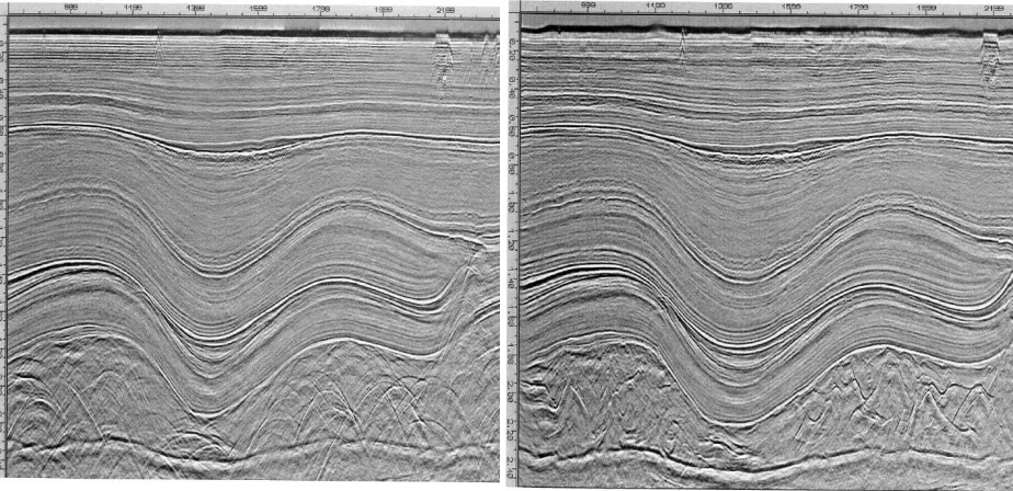
Therefore, necessarily migration should remove the wave propagation artifacts in the output image. The
classic example shown below is from Yilmaz (2001), where the diffractive end-effects from seismic event
termination are removed after migration. In this migration example the dips of the shallow reflectors
are also positioned correctly.
Figure 1 unmigrated section (left), and migrated section (right), from Yilmaz 2001, figure 8.2-28
In an exact migration solution, one would find the inverse of the forward modeling operator and apply it
to the wavefield, generating the reflectivity image, as is shown by equation 3. However, as we can see
from equation 1, because the forward modeling operator is non-orthogonal and non-square, a true
inverse does not exist. To overcome this problem, the adjoint operator is applied, but seismic data are
real (not complex), so the transpose operator may be used. This builds a square matrix, called the
Hessian matrix, which is then inverted and applied to the data.
6
In traditional migration processes this is not done. The inverse Hessian matrix is very large, in fact it is
too large to be handled by modern computers for realistic data sets, so an approximation is made. In the
case of our above example with a 200 gigabyte data set, the inverse Hessian would be 1.3*10^25 bytes.
Multiply by the transpose matrix as above, and the operator becomes 4.7*10^37 bytes. No current
computer is capable of handling arrays this large.
Traditionally, because the inverse Hessian is strongly diagonal it is approximated as being purely
diagonal (Bancroft 2007) and, because the amplitude of the resulting wavefield is qualitative only, an
assumption is made that the inverse Hessian can be approximated as a scalar multiplied version of the
identity matrix. Therefore in traditional migration, a scaled adjoint (really a scaled transpose) is applied
to the data to come up with the reflectivity image. Mathematically, the approximation described above:
(
L
T
L
)
-1
≅ a (
I
)
-1
means equation 4 is now
m = a (
I
)
-1
L
T
d =
L
T
d
(5)where a is a scalar multiplier (which we disregard as unimportant quantitative amplitude information),
and I is the identity matrix.
Iterative modeling and migration (LSM)
LSM attempts to find a true inverse to the forward modeling operator. The Born approximation
demonstrates in the wave equation that a perturbation in the velocity model generates a perturbation
7
(6)
The solution is then obtained via an iterative update of the reflectivity image by minimizing the error
between the predicted (forward modeled) data and the real data. This is done by realizing, as above,
that the wavefield at one source position, us, is linear in the reflectivity
(7)
where Ls is the forward modeling operator for one shot. Also we define a subset of these data, ps,r,
(8)
where Sr, is a receiver station sampling operator. Therefore, the error minimization problem can be
expressed in the following way (Luo 2014)
(9)
where J is the error condition, Es,r is the quantitative error, and ds,r is the real, observed data. The error
condition is our definition of the choice we make to determine the difference between the real and
synthetic datasets. Through use of an iterative conjugate gradient algorithm (Huang 2014), we can move
8
(10)
The goal of LSM is to construct a “true amplitude” image (Plessix 2002), which isn’t possible in reality. In
LSM we generate a solution which is theoretically devoid of errors in the reflectivity image, though in
reality the Born approximation, the acoustic constraint, and the constant density assumption generate
non-zero error (Aki 2002). There is also the question of stability and non-uniqueness of the solution
which will be addressed later in this paper. Gong (2011) discusses the possibility of arriving at a local
minimum in the error conditional, rather than a global minimum. This turns out to be crucial to this
research.
Least squares migration is traditionally constructed on a reverse time migration kernel (Yao 2012; Zhang
2015). It turns out that LSM can actually produce better results when a Kirchhoff migration kernel is
used (Yunsong 2014). This claim will be discussed in the results section of this paper.
The LSM iterative solution is strictly dependent on the input velocity model. Any error in the input
model generates instability in the modeling and migration subprocesses, which can cause the solution to
diverge. The LSM solution drives down the error in the residual image, which is calculated as a wavefield
difference between the forward modeled data and the input (real) data (Wang 2013). With increasing
velocity error in the input velocity model, more LSM iterations are needed to converge to a reflectivity
image solution. If the error in the input velocity model is great enough the LSM solution will become
divergent and thus never reach a stable solution.
In traditional LSM a large bank of stabilizing preconditioning filters is applied to reduce the instability in
the reflectivity image iterations. These stabilizing preconditioners decrease the reflectivity image
9
2014) velocity error, or up to a 10% (Tan 2014) velocity error in the case of vectorized LSM solvers. This
error magnitude is very small; in industrial practice, a 5% velocity error is outstanding in the case of
flawless data acquisition, and unachievable otherwise.
Luo and Hale (2014) were able to produce a crisp LSM image in the presence of a 5% velocity model
error:
Figure 2 Least squares migration of the Marmousi velocity model from Luo and Hale 2014, figure 1-d.
Tan and Huang (2014), using vectorized wavefield separation, were able to produce a crisp LSM image in
10
Figure 3 Least squares migration of the Marmousi velocity model from Tan and Huang 2014, figure 14-b
LSM is an extremely computationally expensive process, and cannot feasibly be completed on data
which has velocity errors significant enough to increase the iteration number dramatically. However,
handled properly LSM pushes seismic images towards true reflectivity models (Zeng 2014).
11
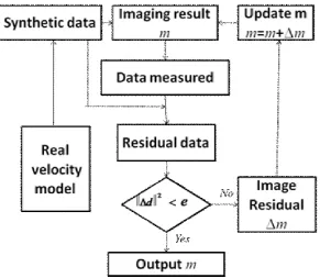
Figure 4 Conventional least squares migration workflow description from Wang 2013, figure 1.
Velocity model updating (full waveform inversion)
After the initial migration of seismic data often the velocity model is updated and the migration run
again to get a better reflectivity image. There are many ways of updating a velocity model, one of which
is full waveform inversion. This technique uses a forward modeling routine to generate a synthetic data
set which is input to another error minimization algorithm. The algorithm automatically updates the
velocity model to change the synthetic data. The model is updated iteratively until a global error
minimum is found between the modeled and real seismic data (Ma 2012).
Pelissier (2008) described the difficulty in inversion based velocity update as “the trade-off between
speed (and robustness) and accuracy.” FWI is extremely computationally expensive, and as such many
FWI algorithms limit the velocity updates to some large threshold value for the error. It is therefore
advisable to somehow limit the error exposure in the input velocity model to the FWI algorithm, which
12
Iterative FWI and LSM (stabilized LSM)
The experiment described in this paper uses FWI as the stabilizing subprocess in an LSM algorithm. The
inputs to the stabilized LSM are the seismic shot records and the initial velocity model. The outputs of
the stabilized LSM algorithm is an optimally updated velocity model and an optimum reflectivity image.
At each iteration in the LSM routine the traditional least squares reflectivity image error minimization
process is applied to the data, forming another more accurate image. Also an FWI subroutine is applied
using updated reflectivity information. The updated velocity model at each step is, at the same time,
input back into the reflectivity image update. This forms a double parallel loop in which error in the
resulting image is reduced at a high rate, and the sensitivity to velocity model error is reduced.
The two benefits of stabilized LSM are decreased velocity error sensitivity and reduction in number of
LSM iterations.Because of the computational cost of conventional LSM, it is not used in industrial
practice (Bancroft 2014). Decreasing the number of required iterations is key to building an algorithm
which can be used on real data. In research and development LSMs velocity sensitivity can be overcome
by simply starting with a more accurate input velocity model. In practice, the true velocity model is
unknown, and therefore velocity error sensitivity is paramount to the application of LSM. Decreasing the
sensitivity of an LSM algorithm is key to building an algorithm which can be used on real data.
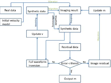
13 Figure 5 Stabilized least squares migration workflow description.
Experiment/Methods
Modeling algorithm
There were two modeling algorithms used concurrently in this experiment. The first is the modeling
algorithm used in the main LSM routine. It is a Kirchhoff depth synthesis algorithm written by the Center
for Wave Phenomena (CWP) at the Colorado School of Mines called “sukdsyn2d”. The algorithm takes
two inputs, a travel time table generated by a ray tracing algorithm and an input migrated seismic
section. The output is the synthetic shot records for the seismic data.
The second modeling algorithm used herein is a finite difference depth algorithm operating on the 2D
acoustic one-way wave equation. This algorithm is the basis for the modeling steps within the FWI
14
the modeling algorithm is wrapped inside a decision making algorithm which performs the velocity
updates on the modified velocity model. This algorithm is explicitly derived from Claerbout (1984).
The runtime of the Kirchhoff depth synthesis algorithm is a small but noticeable contribution to the
overall stabilized LSM speed. Because the modeling algorithm is directly built from the migration
algorithm used in the stabilized LSM, the modeling results are extremely accurate.
The Marmousi velocity model was used in this experiment for completeness. The model is 384 samples
in the x direction, and 122 samples in the z direction. With a sample spacing of 25 meters per sample,
this results in a sythetic velocity model of 9600 meters by 3050 meters. The model is shown below:
Figure 6 Marmousi velocity model, red is 5500 m/s, dark blue is 1500 m/s.
Running the finite difference forward modeling algorithm used in this paper on the Marmousi velocity
15
Figure 7 Brute stack corresponding to the Marmousi velocity model of Figure 6.
The modeling algorithm outputs shot gathers for use in the LSM workflow, but for demonstration the
above data have been corrected for geometrical spreading using a time-squared correction factor,
filtered with a wide open bandpass Ormsby frequency-domain filter, and stacked with a constant lateral
velocity normal moveout correction.
Migration algorithm
The migration algorithm used in this experiment is a standard Kirchhoff depth migration, developed by
CWP, called “sukdmig2d”. The migration operator is built in the standard way and approximates a scaled
transpose (as described in the migration subsection of the background section of this paper) to the
modeling operator used in the LSM routines in this research.
Several finite difference migration operators (based on Bruno, 2011) were developed in preparation for
the stabilized LSM with promising imaging results. However, because of the duality of the modeling and
16
LSM image. The results which produced resolution high enough for analysis were the results using the
above mentioned sukdmig2d operator. The inverse relationship between the modeling and migration
operators ensures the high degree of spatial resolution demonstrated in the results section.
The experiment used a standard migration algorithm on each velocity model as a control. Running a
standard migration is equivalent to running an LSM algorithm with zero iterations, because there is no
reflectivity image update in one iteration of LSM, just one migration. For completeness it was necessary
to demonstrate the resolution difference between a standard migration and an LSM. It was preferable
to run the same type of migration as exists in the LSM routine, in this case the exact same code.
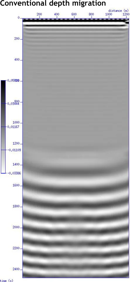
For demonstration this migration algorithm was run on the modeled gathers of the above image, with
the following output:
17
Again the output has been conditioned for clarity. After migration the image was automatically gain
controlled with a time gate of 1000 milliseconds, trace balanced on a root mean square amplitude basis,
lightly FX deconvolved using a trace window of 50 traces, and clip gained at 99%.
FWI algorithm
The FWI algorithm in this experiment is a custom code developed by Sandstone Oil & Gas called
“ssogfwi”. It uses a cross correlation based comparison function to build a difference model based on
the 2D power spectral density. The main function in this program is a decision making algorithm which
makes decisions about which direction to update the velocity model based on changes in the modeled
wavefield. The algorithm iterates through shots and depth steps to minimize the error at each lateral
position on the seismic line and each depth step in a shot. The comparison function takes the whole
shot gather at one time, therefore it is a true FWI program. As opposed to tomographic velocity update
techniques, FWI does actually contain information about all wavelengths (Tang 2013).
Out of all of the subprocesses in the stabilized LSM program, the FWI runs the slowest, which is to be
expected. Because this subprocess must analyze the whole data set at one time, the speed is nonlinear
with respect to both the depth and the lateral extent domains. In the future the FWI code, and thus the
stabilized LSM, could be optimized in the wavenumber domain (Bracewell 2000) which would increase
the speed by an estimated factor of 1000 times for the FWI, resulting in an estimated increase in speed
of 10 times for the stabilized LSM. The use of wavelet decomposition (Strang 1997, Miller 2004) might
also enhance the speed of the FWI.
Automatic batch controller (the LSM brain)
The LSM routine is built in the style of a Unix batch controller. It batches out subprocesses to the CPU
cores by monitoring the load state of the processors. The flow control is built into a double parallel loop
which simultaneously updates the velocity model via FWI (the loop on the left side of Figure 5) and the
18
connected to stabilize the LSM at two points. The first pipes the updated image modeled data back into
the velocity update, and the second pipes the returned updated velocity model and the output shot
gather data stream back into the conventional LSM routine.
The inclusion of the updated velocity model in the reflectivity image update is a stabilizing feature which
is unique to this research. The shot gather balance reinjection into the conventional reflectivity update
was an alternative approach to a small stabilizing preconditioning filter bank. This procedure is much
more natural than applying an arbitrary filter bank, as it uses the output of the velocity update loop to
implicitly stabilize the shot gather data before the residual image calculation.
The inclusion of an automated batch controller was preferential to a fully parallel build in one large
C/C++ based program. There are two reasons for this choice. First, from a research standpoint, it makes
more sense to build a system which is easily piecewise modifiable. This is because you can generate
perfectly reproducible results from the entire stabilized LSM algorithm, save for the change in one
subprocess which one uses to test results. Second, more importantly, the batch architecture is
completely modular. To improve results, a future researcher can simply plug in a more sophisticated
migration algorithm, or to test a new stabilization routine, a processor could replace the current FWI
with a custom product.
Experiment
Three processes were run: first the simple Kirchhoff depth migration, second the conventional LSM, and
third the stabilized LSM. These processes were tested using the correct velocity model and three
velocity models with different types of error.
The data tested were synthetic data generated by finite difference forward modeling a small velocity
model, at 50 traces by 100 samples at 25 meter spacing in each direction. This corresponds to a model
19
line, which for example could be 16,000 meters by 12,000 meters, or 192 million square meters, this
experiment is running a data set which is 1.6% of a real data set.The sample data set took an average of
10.5 days to run at 6 iterations.
The first data tested were forward modeled from a simple, heterogeneous two velocity model. The
20 Figure 9 Correct two velocity homogeneous velocity model.
There were three types of error introduced: first a scalar shift to the entire velocity model, second a
homogeneous lateral error layer in the first velocity, and third a laterally heterogeneous velocity block.
Each one of the velocity errors was varied from one to ten percent of the total maximum velocity in the
model. The error magnitude in the images below is ten percent, as to visually highlight the region of
21
22
23
Figure 12 Two velocity homogeneous velocity model with a ten percent lateral velocity error.
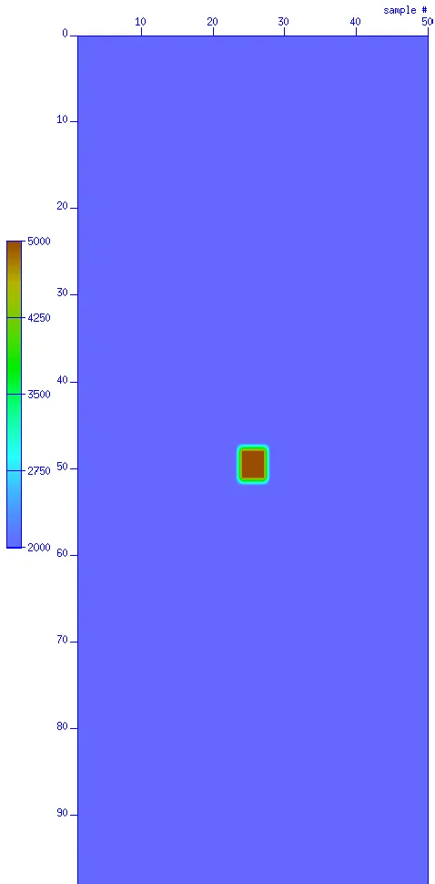
The second data tested was on an impulse response velocity model. The background medium has a
25
26
27
Figure 16 Impulse response velocity model with a ten percent lateral velocity error.
The third velocity model tested was a two velocity laterally heterogeneous velocity model. The upper
medium has a velocity of 2000 meters per second and the bottom medium has a velocity of 4000 meters
28
29
30
31
Figure 20 Two velocity laterally heterogeneous velocity model with a ten percent lateral velocity error.
The second part of the experiment included half of the Marmousi velocity model. With a horizontal and
vertical sample spacing of 25 meters, the 192 by 122 sample Marmousi model comes out to a total of
32
a considerable portion of memory; running at peak efficiency requires about 64GB of memory by the
end of each iteration.
33
Figure 22 Western half of the Marmousi velocity model with a ten percent lateral velocity error.
These velocity errors typify and isolate the error encountered in real velocity modeling. Scalar
inconsistencies in velocity modeling are generated due to an incorrect starting velocity model, as in the
process of brute stacking. Laterally continuous velocity errors isolated in vertical extent are
representative of the error in velocity models due to an incorrect high or low pick on a semblance plot,
including those erroneous picks due to multiple energy. This type of velocity error is also encountered in
automated velocity update schemes, wherein a velocity updating algorithm assigns an incorrect
degenerate velocity to a specific data layer (or group of layers). Laterally discontinuous velocity errors
can be the result of many factors, with the most common factor being the spatial averaging of
inconsistent human velocity picks across multiple CMP locations. This occurs when a velocity interpreter
picks an erroneously high or low velocity with respect to the surrounding gross grid locations, as then
the velocity interpolation scheme spreads that error to the adjacent CMP locations with error
34
Results
Modeled data (correct velocity model)
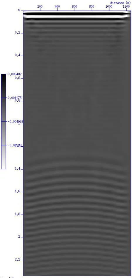
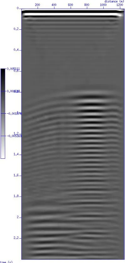
The following data are the result of running the above mentioned finite difference forward modeling
algorithm on the correct velocity model listed below. These images should give the reader an
understanding of the starting point of the data before viewing the results of the migrations in
subsequent sections.
35
36
37
38
39
40
Figure 29 Common shot gathers modeled from the Marmousi velocity model.
41
Conventional depth migration
42
43
44
45
46
47
48
49
50
51
52
53
54
55
56
57
58
59
60
61
62
63
64
65
66
67
68
69
70 Figure 60 Correct Marmousi Kirchhoff depth migration section.
71
Conventional LSM
72
73
74
75
76
77
78
79
80
81
82
83
84
85
86
87
88
89
90
91
92
93
94
95
96
97
98
99
Stabilized LSM
100
101
102
103
104
105
106
107
108
109
110
111
112
113
114
115
116
117
118
119
120
121
122
123
124
125
126
127
All of the images in this chapter have excluded any post processing to highlight any numerical
inconsistencies in the solutions. All of the images in this section are the outputs from the stabilized LSM
algorithm. The color images on the left are the updated velocity models and the images on the right are
the updated seismic sections. They are both set at the same scale for visual comparison. Compare the
results in this section with the results in the depth migration section in this chapter to visualize the
resolution enhancing ability of the stabilized LSM.
Analysis
Iteration comparison
The following three figures are comparisons of iterations taken to minimal error condition. The
horizontal axis code is structured as follows: the first two letters correspond to homogeneous, impulse,
or heterogeneous velocity model, the middle numbers correspond percentage error, and the last two
128
129
130
Figure 120 Number of iterations sorted by velocity model error type (lateral, scalar, and stripe)
In figures 118 - 120, the impulse response velocity model exhibits an anomalously large change in
iteration number between conventional LSM and stabilized LSM because the stabilized LSM did not
resolve the velocity anomaly. Each iteration of the stabilized LSM washed out more and more of the
correct velocity model, implying that the best image was output after one iteration.
Velocity Sensitivity
The conventional LSM destabilized in the following cases, all models with ten percent velocity error: the
homogenous velocity model with all three types of velocity error and all four velocity models with
lateral velocity error. This is indicative of a higher degree of velocity sensitivity in the lateral dimension
than the vertical dimension. Because the FWI algorithm which stabilizes the stabilized LSM updates the
velocity at each iteration in two dimensions, there was no destabilization in these results from the
131
For completeness, in the course of this research the stabilized LSM algorithm was tested to the point of
failure with respect to the maximum stable velocity error. During this torture testing, the stabilized LSM
tested stable up to 18% velocity error for lateral velocity errors, and up to 23% for laterally continuous
velocity errors (including scalar errors).
Reflectivity error resolution
As is demonstrated in the results above, the reflectivity error minimization improves the overall quality
of the seismic section more than the velocity error minimization. This is evident when comparing the
depth migrated sections above to the stabilized LSM images and when comparing the depth migrated
sections to the conventional LSM images. The improvement in image quality between these two steps is
much more pronounced than the improvement in image quality between the conventional LSM and the
stabilized LSM. This is to be expected, as the stabilized LSM image quality should be on the same order
of magnitude as the conventional LSM.
A comparison of the reflectivity error resolution between the stabilized LSM and the conventional LSM
demonstrates the ability of the stabilized LSM to produce an output image with higher reflectivity
accuracy than that of the conventional LSM. This is evident along the left side of the velocity anomaly
where we see seismic events with a higher degree of lateral continuity in the stabilized LSM output than
the conventional LSM output. The false anticline below the right side of the velocity anomaly in both of
these images is also evident, however, in the stabilized LSM output the vertical displacement of the
anticline is less severe. Lastly, the stabilized LSM output images the high velocity wedge layer below the
velocity anomaly with increased vertical and lateral resolution as compared to the conventional LSM.
Velocity solution uniqueness
The updated velocity sections output from the stabilized LSM suffer from lateral banding artifacts as
seen in all of the output velocity models. This is due to the non-unique wavefield structural dependency
132
characteristics from two different input velocity models. An input velocity model with a paired
anomalously high and anomalously low lateral velocity inconsistency can forward model with the same
wavefield structure as a correct velocity model input as long as the vertical extent of the inconsistencies
is not located on a lateral change in the velocity model. This is shown in every updated velocity section
from the stabilized LSM above, but it is especially noticeable in the two velocity homogeneous velocity
models (aside from the ones with lateral velocity errors) obviously because there are no lateral changes
in velocity.
However, the amplitudes in the output seismic section from the stabilized LSM do not exhibit the same
amplitude characteristics as that in the conventional LSM. Intuitively, this makes sense; if the vertical
extent of the velocity inconsistency is shorter than a quarter of the dominant wavelength there would
be no effect on the output wavefield, but as the inconsistency grows in vertical length the wavefield will
exhibit an increased amplitude distortion.
The above does not hold for laterally discontinuous velocity features. The lateral velocity error bands in
the updated velocity model do destroy laterally isolated velocity artifacts in a correct model. The
evidence for this is in the impulse response velocity sections, wherein the wavefield solution does not
diverge, but the impulse square is washed out of the image with each iteration of wavefield update.
Velocity error resolution
In all cases, the input velocity errors were reduced in magnitude. However, velocity errors were
generated in lateral bands across the velocity sections. The velocity error resolution is most pronounced
in the cases of lateral velocity error in the two velocity homogeneous and the two velocity
heterogeneous models. In the cases of the five percent velocity errors the error was reduced by up to
65% for the homogenous velocity model and 68% for the heterogeneous model. In the cases of the ten
133
for the heterogeneous model. In the case of the Marmousi velocity model, the stabilized LSM corrects
the velocity almost to the point of human perception. While the actual, quantitative correction is the
same as the other lateral velocity error corrections, this experiment shows the effective velocity error
resolving effect on real data.
Conclusions
Conventional LSM vs. Stabilized LSM
Figure 121 Iteration comparison after removing the divergent solutions in conventional LSM and the impulse response velocity models which were not accurately resolved by the stabilized LSM.
In the above figure we see a fair comparison between the conventional LSM and the stabilized LSM. In
this figure the divergent conventional LSM solutions have been removed and the impulse response
velocity model stabilized LSM solutions have been removed. In only two cases did the conventional LSM
134
cases the stabilized LSM minimized reflectivity image error with fewer iterations than the conventional
LSM. This showcases the ability of the stabilized LSM to run on real data in the near future.
The inclusion of the stabilizing routine in the LSM generated lateral velocity artifacts in the velocity
output. However, because of the dual error minimization subroutines in the stabilized LSM the image
solution was improved. This is because the velocity artifacts generated in the velocity update iterations
are annealed by the reflectivity update iterations. The output images would certainly be even more
accurate without the generation of velocity errors in the FWI function, so future work must be done to
include a lateral error reduction subroutine into the FWI function.
The inclusion of FWI as a stabilizing agent in the LSM solution is effective. The results from the stabilized
LSM came back with similar or better resolution than the results of the conventional LSM. The use of
FWI stabilized the imaging solutions for the Marmousi velocity model up to a 19% velocity error, which
is larger than conventional stabilizing preconditioning banks. In each case the algorithms had trouble
with lateral resolution of lateral reflectivity discontinuities, but this can be fixed by using a different
migration algorithm with a sharper lateral impulse response. The design of both the stabilized and the
conventional LSM algorithms in this paper permit this change easily, as described in the next section.
Modular algorithm - imaging resolution
As was discussed in the methods chapter, the stabilized LSM algorithm used in this research is fully
modular. Each subprocess contained in the stabilized LSM controller can be swapped for another
algorithm. The huge benefit here is that to improve imaging accuracy all one would need to do is plug in
a different modeling algorithm or a different migration algorithm.
As demonstrated in the results chapter, the modeling algorithm in this research generates a non-trivial
amount of numerical noise in its output. This could easily be corrected by plugging a more advanced
135
by modern standards. The inclusion of a modern depth migration, especially a finite difference
migration, would significantly improve the imaging resolution of the stabilized LSM.
As an additional appendix to this paper, the source code, in its entirety, is located on a private software
136
Bibliography
● Aki, Keiiti. Richards, Paul G. Quantitative Seismology, 2nd ed. University Science Books, 2002. ● Amaro, Bruno. Et. Al. “A comparison of stabilized least-squares imaging conditions for
wave-equation migration”. Sociedade Brasileria de Geofisica, 2011. SBGf2011: 1065-1069.
● Bacon, M. et al. 3-D Seismic Interpretation. New York, NY: Cambridge University Press, 2007. ● Bancroft, John C. A Practical Understanding of Pre- and Poststack Migrations. Course Notes
Series, No. 14. SEG, 2007.
● Bancroft, John C. SEG Continuing Education Course. “A Practical Understanding of Inversion for Exploration Geophysicists”. Continuing Education Series, 2014.
● Bishop, T.N. Et. Al. (June 1985). “Tomographic determination of velocity and depth in laterally varying media”. Geophysics 50 (6): 903-923.
● Bracewell, Ronald N. The Fourier Transform and Its Applications. Singapore: McGraw-Hill, 2000. ● Chu, Chunlei. Et. Al. (October 2010). “Frequency domain modeling using implicit spatial finite
difference operators”. SEG Denver 2010 Annual Meeting. SEG Expanded Abstracts, 2010: 3076-3080.
● Claerbout, Jon F. Imaging the Earth’s Interior. Stanford Exploration Project, 1984.
● Dutta, Gaurav. Schuster, Gerard T. (November 2014). “Attenuation compensation for least-squares reverse time migration using the viscoacoustic-wave equation”. Geophysics 79 (6): S251-S262.
● Gong, Bin. Shen, Yunqing. (October 2011). “Full Waveform Inversion with Reflection Energies”. SEG San Antonio 2011 Annual Meeting. SEG Expanded Abstracts, 2011: 2439-2443.
● Hilterman, Fred. Graul, Mike. SEG Continuing Education Course. “Seismic Lithology”. Continuing Education Series, 2009.
● Huang, Tunsong. Et. Al. (September 2014). “Making the most out of least-squares migration”. The Leading Edge: 954-960.
● Huang, Wei. Zhou, Hua-Wei. (October 2014). “Stochastic conjugate gradient method for least-square seismic inversion problems”. SEG Denver 2014 Annual Meeting. SEG Expanded Abstracts, 2014: 4003-4007.
● Ji, Jun. (November 1997). “Tomographic velocity estimation with plane-wave synthesis”. Geophysics 62 (6): 1825-1838.
● Jin, Shenwen. Et. Al. (October 2014). “Structure tensor constrained tomographic migration velocity analysis”. SEG Denver 2014 Annual Meeting. SEG Expanded Abstracts, 2014: 4702-4706. ● Liu, Yang. (October 2012). “Finite-difference modeling with a minimal computation cost”. SEG
Las Vegas 2012 Annual Meeting. SEG Expanded Abstracts, 2012: 1-5.
● Liu, Yang. Sen, Mrinal K. (July 2011). “Finite-difference modeling with adaptive variable-length spatial operators”. Geophysics 76 (4): T79-T89.
● Luo, Simon. Hale, Dave. (July 2014). “Least-squares migration in the presence of velocity errors”. Geophysics 79 (4): S153-S161.
● Ma, Yong. Et. Al. (August 2012). “Image-Guided Sparse-Model Full Waveform Inversion”. Geophysics 77 (4): R189-R198.
● Marfurt, Kurt J. Chopra, Sattinder. Seismic Attributes for Prospect Identification and Reservoir Characterization. Tulsa, OK: Society of Exploration Geophysicists, 2008.
● Meunier, Julien. 2011 Distinguished Instructor Short Course. “Seismic Acquisition from Yesterday to Tomorrow”. Distinguished Instructor Series, No. 14: Society of Exploration Geophysicists, 2011.
137
● Pelissier, Michael A. Prestack Depth Migration and Velocity Model Building. SEG, 2008. ● Plessix, Rene-Edouard. Mulder, Wim. (October 2002). “Amplitude-preserving finite-difference
migration based on a least-squares formulation in the frequency domain”. SEG Int’l Exposition and 72nd Annual Meeting.
● Ryan, Harold. “Ricker, Ormsby, Klauder, Butterworth – A Choice of Wavelets”. Hi-Res Geoconsulting. Canadian Society of Exploration Geophysicists. September 1994.
<http://www.cseg.ca/publications/recorder/1994/09sep/sep94-choice-of-wavelets.pdf> ● Sheriff, Robert E. Encyclopedic Dictionary of Exploration Geophysics. Tulsa, OK: Society of
Exploration Geophysicists, 1991.
● Strang, Gilbert. Nguyen, Truong. Wavelets and Filter Banks. Wellesley MA: Wellesley-Cambridge Press, 1997.
● Tan, Sirui. Huang, Lianjie. (September 2014). “Least-squares reverse-time migration with a wavefield-separation imaging condition and updates source wavefields”. Geophysics 79 (5): S195-S205.
● Tang, Yaxun, Et. Al. (October 2013). “Tomographically enhanced full wavefield inversion”. SEG Houston 2013 Annual Meeting. SEG Expanded Abstracts, 2013: 1037-1041.
● Tarantola, Albert. (August 1984). “Inversion of seismic reflection data in the acoustic approximation”. Geophysics 49 (8): 1259-1266.
● Telford, W.M., et al. Applied Geophysics, 2nd ed. New York, NY: Cambridge University Press, 1990.
● Upadhyay, S.K. Seismic Reflection Processing with Special Reference to Anisotropy. Berlin, Germany: Springer-Verlag, 2004.
● Wang, Xiaotian. Et. Al. (October 2013). “The Least-squares Pre-stack Fourier Finite-difference Migration”. SEG Houston 2013 Annual Meeting. SEG Expanded Abstracts, 2013: 3926-3930. ● Yao, Gang. Jakubowicz, Helmut. (October 2012). “Least-Squares Reverse-Time Migration”. SEG
Las Vegas 2012 Annual Meeting. SEG Expanded Abstracts, 2012: 1-5.
● Yilmaz, Oz. Seismic Data Analysis. Investigations in Geophysics, No. 10. SEG, 2001.
● Zeng, Chong. Et. Al. (September 2014). “Least-squares reverse time migration: Inversion-based imaging toward true reflectivity”. The Leading Edge: 962-968.
● Zhan, Ge. Schuster, Gerard. (October 2010). “Skeletonized Least Squares Wave Equation Migration”. SEG Denver 2010 Annual Meeting. SEG Expanded Abstracts, 2010: 3380-3384. ● Zhang, Yu. Et. Al. (February 2015). “A stable and practical implementation of least-squares
138
Appendix – stabilized LSM algorithm
Included below is the source code for the stabilized LSM algorithm. The full source code for all of the
software in this research is available by request from a private repository. The results in their entirety
(over 1000 data sets) are also available at a separate online repository. If you would like access, please