Detecting cancer clusters in a regional population with local cluster tests and Bayesian smoothing methods: a simulation study

(1)

R E S E A R C H

Open Access

Detecting cancer clusters in a regional population

with local cluster tests and Bayesian smoothing

methods: a simulation study

Dorothea Lemke

1,2*

, Volkmar Mattauch

3

, Oliver Heidinger

3

, Edzer Pebesma

2

and Hans-Werner Hense

1,3

Abstract

Background:There is a rising public and political demand for prospective cancer cluster monitoring. But there is little empirical evidence on the performance of established cluster detection tests under conditions of small and

heterogeneous sample sizes and varying spatial scales, such as are the case for most existing population-based cancer registries. Therefore this simulation study aims to evaluate different cluster detection methods, implemented in the open soure environment R, in their ability to identify clusters of lung cancer using real-life data from an epidemiological cancer registry in Germany.

Methods:Risk surfaces were constructed with two different spatial cluster types, representing a relative risk of RR = 2.0 or of RR = 4.0, in relation to the overall background incidence of lung cancer, separately for men and women. Lung cancer cases were sampled from this risk surface as geocodes using an inhomogeneous Poisson process. The

realisations of the cancer cases were analysed within small spatial (census tracts, N = 1983) and within aggregated large spatial scales (communities, N = 78). Subsequently, they were submitted to the cluster detection methods. The test accuracy for cluster location was determined in terms of detection rates (DR), false-positive (FP) rates and positive predictive values. The Bayesian smoothing models were evaluated using ROC curves.

Results:With moderate risk increase (RR = 2.0), local cluster tests showed better DR (for both spatial

aggregation scales > 0.90) and lower FP rates (both < 0.05) than the Bayesian smoothing methods. When the cluster RR was raised four-fold, the local cluster tests showed better DR with lower FPs only for the small spatial scale. At a large spatial scale, the Bayesian smoothing methods, especially those implementing a spatial neighbourhood, showed a substantially lower FP rate than the cluster tests. However, the risk increases at this scale were mostly diluted by data aggregation.

Conclusion:High resolution spatial scales seem more appropriate as data base for cancer cluster testing and monitoring than the commonly used aggregated scales. We suggest the development of a two-stage approach that combines methods with high detection rates as a first-line screening with methods of higher predictive ability at the second stage.

Keywords:Spatial cancer cluster, Local cluster tests, R, DCluster, Bayesian smoothing methods, Simulation design, Epidemiological cancer registry

* Correspondence:[email protected]

1_{Institute of Epidemiology and Social Medicine, Medical Faculty, Westfälische} Wilhelms-Universität Münster, Albert-Schweitzer-Campus 1 D3, D 48149, Münster, Germany

2

Institute for Geoinformatics, Geosciences Faculty, Westfälische Wilhelms Universität Münster, Münster, Germany

Full list of author information is available at the end of the article

INTERNATIONAL JOURNAL OF HEALTH GEOGRAPHICS

© 2013 Lemke et al.; licensee BioMed Central Ltd. This is an open access article distributed under the terms of the Creative Commons Attribution License (http://creativecommons.org/licenses/by/2.0), which permits unrestricted use, distribution, and reproduction in any medium, provided the original work is properly cited.

(2)

Background

The introduction of a prospective and systematic cluster monitoring has been debated in Germany for a long time [1]. The German state of Lower Saxony is currently considering the introduction of such a monitoring sys-tem because unexplained incidence elevations have been observed for various cancer sites in the municipality of Asse which hosts a nuclear waste repository [2]. It is current practice in the German epidemiological cancer registries that only “event related” cluster investigations are conducted. These respond to requests from the pub-lic, from medical doctors or health departments and arise on the basis of suspected putative cancer clusters in certain, mostly small, spatial areas. Statistical testing in these cases usually involves the estimation of stan-dardized incidence ratios (SIR), that is, the ratio of the cases of a certain malignant entity in a given area in rela-tion to the number expected on the basis of the rates for this cancer type in an appropriate reference population. If the SIR rise is statistically significant, a cluster is sus-pected and further investigation is needed to verify an association with a specific source of exposure [3].

A cluster is commonly defined as a geographically confined group of cancer cases of sufficient size that are unlikely to have occurred by chance [4]. However, this approach has serious methodological limitations: On the one hand, no hypothesis driven analyses are possible since the clusters are detected before the hypothesis of elevated cancer risk areas is formulated (also known as Texas sharpshooter fallacy) [5]. On the other hand, there is a substantial multiple testing problems given the multitude of tests (different communities, different time periods, different cancer diagnoses) that must be per-formed. More importantly, such event-driven cluster in-vestigations rarely discover smaller or weaker exposure related clusters nor do they help to identify novel etio-logic associations [6,7]. By contrast, extensive small-scale monitoring (or prospective cluster monitoring) avoids many of these problems, in particular the post-hoc bias introduced by finding a cluster in randomness. There-fore, a data and hypothesis driven analysis should be preferred employing the whole spatial and temporal ex-tent of registry data. Additional benefits may be seen in a better use of the full set of cancer registry data which is one major purpose for running cancer registries. Moreover, a monitoring that covers a complete region has advantages in terms of not only screening the puta-tive exposure-associated tumours over time and space but to encompass also other cancer sites which are re-lated to differential spatial distributions. Thus, the spatial incidence patterns of tumours, like breast and prostate cancer, can indicate how screening behaviour varies over space and time. Monitoring can also provide data about the spatial and temporal variation of lifestyle associated

tumours that belong to certain risk behaviours (like alco-hol or tobacco consumption).

Spatially focussed data may therefore have important im-plications for public health policies. To conduct compre-hensive and extensive spatial risk monitoring programs, various methods have been made available that range from local cluster tests to full Bayesian smoothing methods [5]. Usually, there is no a priori knowledge about the location of“true”clusters in the application of such methods.

This study was planned and conducted with the aim of evaluating the performance of commonly used local cluster tests and Bayesian smoothing methods in terms of their detection and prediction rates when applied in a simulated spatial risk surface. The second aim of the study was to assess the spatial resolution of the methods, that is, to test on which spatial scale clusters are still suf-ficiently identifiable. The spatial units used were 78 communities and 1983 census tracts. The community level is the lowest spatial unit in the common adminis-trative division of Germany and corresponds to the LAU 2 (level of local administrative units) in the EU. There exist several simulation studies that evaluated the statis-tical performance of cluster detection tests [8-14] but only few investigated the performance of these tests when using different spatial aggregation level [9,10,15]. Most of these simulation studies were designed for set-tings with huge sample sizes (10 000-50 000 cases) which cannot be directly compared to the conditions de-scribed above where cancer registries deal with much smaller samples sizes and a lower spatial resolution of the administrative data. We aimed to investigate the ac-curacy and precision of cluster detection tests and Bayesian smoothing techniques when applied to a set-ting with smaller areas, lower population numbers and fewer cancer cases. For this simulation study a common type of cancer, lung cancer in men and women in the age group between 40 and 79 years, was chosen as sam-ple data.

Data and methods

Study area

(3)

Simulation design

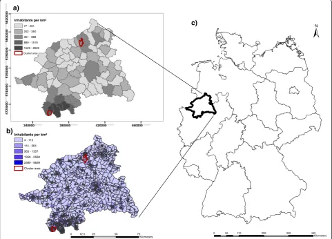
For this simulation study, lung cancer (ICD-10: C34) cases occurring in men and women in the age group be-tween 40 and 79 years were chosen as sample data. Spatial cancer risk surfaces were constructed by arbitrar-ily defining two artificial cluster areas at the level of the census tracts. Within these cluster areas, two magni-tudes of risk elevation were applied such that the lung cancer risk was computationally set to be either two-(RR1= 2.0) or four-fold (RR2= 4.0) as high as the

ob-served risk. The two risk areas were nested within larger communities. The northern cancer cluster (encompass-ing 6 of the total 50 census tracts in that community) had more rural characteristics, that is, a larger area and lower population density. The second cancer cluster was generated in the south (encompassing 37 out of a total of 99 census tracts composing the entire community) with more urban characteristics, that is, a smaller area and units with higher population density (Figure 1).

The expected numbers of cancer cases (Ei) per census

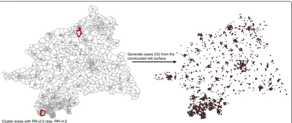
tract were estimated employing the age-standardized in-cidence rate for lung cancer as obtained from the data-base of the epidemiological cancer registry of North Rhine-Westphalia [18]. The observed cases (Oi) were

sampled from the four constructed risk surfaces (urban & rural cluster with either RR1= 2.0 or RR2= 4.0) as

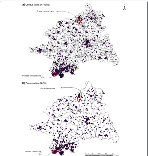
geo-codes using an inhomogeneous Poisson point process (Figure 2). 1000 realisations of the process for each clus-ter and RR magnitude were generated using function rpoispp from the R package spatstat. These realisations (Oi) were aggregated within census tracts and

communi-ties, respectively, and used for the subsequent local clus-ter tests and Bayesian smoothing methods (Figure 3).

Local cluster tests

Local cluster tests aim to provide information about the spatial location of suspected clusters. The statistical con-cept behind the local cluster tests rests on the assumption

340000.000000 ₃₈₀₀₀₀.000000 ₄₂₀₀₀₀.000000 ₄₆₀₀₀₀.000000

5

720

000

.000

0

0057

40

000

.00

00

0057

6

00

0

.00

00

00578

0

000

.0

0

00

0

0₅₈₀₀

000

.000

0

0₅₈2

00

0

.000

0

00

0 55 110 220 330 440

Kilometers

0 12.5 25 50 75

Kilometers a)

b)

c)

Inhabitants per km²

4 - 113

114 - 564

565 - 1357

1358 - 2588

2589 - 9839

Cluster area

Inhabitants per km²

77 - 201

202 - 350

351 - 888 889 - 1519

1520 - 2622

Cluster area

Figure 1Overview of the study area (Regierungsbezirk Münster) with the modelled cluster areas.Two different spatial aggregation scales are shown:(a)the 78 communities and(b)the 1983 census tracts with the associated population density. Location of the study area in Germany(c).

Lemkeet al. International Journal of Health Geographics2013,12:54 Page 3 of 18

(4)

that disease risk is constant across the study population (constant risk hypothesis or null hypothesis, implying identical risk for each individual). The standardized inci-dence ratio (SIR), defined as ratio of observed to expected cases, is commonly used as a measure of relative disease risk. A constant risk implies that SIR = 1.0. A SIR value that is significantly larger than 1 indicates a disease clus-ter. Two types of local cluster tests were applied: The first is based on local measurements of spatial autocorrelation (local Moran’s I) and the second is based on variously de-fined windows that scan the study region for elevated dis-ease risk (Kulldorff spatial scan statistic; Besag & Newell) [19]. We applied the methods provided in the R packages DCluster (version 0.2-2) [20] and spdep [21]. For local Moran’s I, Kulldorff spatial scan statistic, and the method of Besag & Newell [20], all computations were performed with R version (2.13.1) [22].

- Local Moran’s I

The local Moran’s I measures the deviations of a value in comparison to the mean of the neighbouring areas. In this study, the standardized residuals, as defined in [5], were used. At census tract level, a significantly positive statistic of I (p-value≤0.05) was used in order to detect adjacent census tracts of high risk (hot spot clustering). By contrast, at community level, significantly negative values of I (p-value≤0.05) were considered because here the aim is detection of communities that deviate ex-tremely from neighbouring communities (local outliers). The R-function localmoran from R package spdep [21] was used under the assumption of normality and through the randomisations approach [5]. Due to the small number of spatial neighbours at community level,

the exact (localmoran.exact) form of the standard devi-ates were calculated because the assumption of the nor-mal distribution potentially lead to errors of inference [23,24]. The p-values were adjusted for multiple testing using the false discovery rate (FDR) [25]. This criterion controls the expected proportion of false discoveries among the rejected hypotheses and has been found to be more powerful in the detection of spatial clusters than the family-wise error rates [26]. The FDR approach is implemented in the R-function p.adjustSP from the package spdep [21] which additionally adjusts by ac-counting for spatial neighbours: the p-values are based on the number of neighbours (+1) of each region, rather than the total number of regions.

- Kulldorff’s spatial scan statistic

The Kulldorff spatial scan statistic [27] is based on the likelihood ratio statistics. In this approach, a variable cir-cular scan window was applied to the study area, with radius increasing up to 50% of the population at risk. The actual likelihood ratio is calculated for each circle as the ratio of observed to expected cases within and outside the scan window (Lactual). The likelihood

func-tion assuming Poisson distributed cases is proporfunc-tional to:

c E c½

c

C−c C−E c½

C−c

I cð >E c½ Þ ð1Þ

where c is the number of cases, E[c] is the expected number of cases within a circle and (C-c) and (C-E(c)) the observed and expected cases outside the scan window. We chose the indicator function to be 1.0 if the observed Generate cases (Oi) from the

constructed risk surface

Cluster areas with RR=2.0 resp. RR=4.0

(5)

number of cases was higher than expected. Under the null hypothesis, assuming a constant risk over the study area, datasets are generated and the maximum likelihood ratio (L0) is saved. The statistical significance is computed by

means of Monte-Carlo simulation and yields the probabil-ity that Lactual is exceeded anywhere in the study area;

clusters least consistent with the null hypothesis are

highlighted. The Kulldorff spatial scan statistic adjusted for the multiple testing by the use of one test only. The analyses were conducted with functionopgamfrom the R package DCluster [20], the significance was defined at the 0.05 level and the p-values were calculated using 9999 Monte-Carlo realizations. The most likely clusters were considered with a p-value≤0.05.

a) Census tracts (N=1983)

b) Communities (N=78)

37 urban census tracts

6 rural census tracts

1 rural community

1 urban community

0 5 10 20 30 40

Kilometers

Figure 3Spatial aggregation scales of the realised observed cases.The observed cases (Oi) were aggregated to the census tracts(a), and to

the communities(b).

(6)

- Approach of Besag & Newell

In the method of Besag & Newell [28] the scan window is defined by the number of enclosed cases (k). In the case of rare diseases, like cancer, the number of enclosed cases varies between 2 and 10 [19]. This approach evalu-ates the probability whether the specified k cases are ob-served in fewer regions [5]. To this end, the actual number of regions (li) is compared with the number of

regions under the constant risk hypothesis (Li) using a

Poisson distribution (1-Pr(Li ≤ li) ~ Poisson(Ei)). The

analyses were made with the R function opgamR pack-age DCluster [20] and the p-values were adjusted using the FDR approach implemented in the R-function p.ad-just from the package stats [29]. The number of k enclosed cases was arbitrarily chosen and we used kCT=

5, kCT = 10, kCT = 13 for census tracts and kcom = 15,

kcom= 20, and kcom= 30 for communities.

Bayesian smoothing methods

Smoothing methods do not primarily detect clusters. Their aim is to model/estimate the spatial distribution of the true underlying disease risk because mapping the crude SIR has major drawbacks, especially the instability of the estimates in region with low background popula-tion. Smoothing methods therefore try to remove the random noise caused by the unstable estimates. It is also possible to deploy these smoothing methods in the field of cancer surveillance with the aim to identify risk areas.

- Empirical Bayes smoothing

The Bayesian smoothing methods define the risk meas-ure as a random variable and therefore assign a distribu-tion to the estimate of the“true”risk (= theta(θi)). In the

empirical procedures, the parameters defining this risk distribution (= priors) are estimated from the data. The estimates of theta were stabilized through borrowing in-formation from the prior mean. The amount of strength borrowed depends on the stability of the crude local SIR (or risk measure) as measured by the prior variance [5].

Three models were applied: two global (non-spatial) models (Poisson-Gamma (PG) model and log-normal model) with smoothing the risk estimates towards the global mean, and a local (spatial) model that smoothes the risk to a spatial neighbourhood mean. Both global models were implemented in the DCluster R package [20] and the local model in the spdep package [21]. The PG-model assumes that the observed cases (Oi) are

Pois-son distributed and because it is likely that the counts (Oi) are overdispersed, it is reasonable to define theta as

Gamma distributed withθi~ Gamma(α,β). The priors α

(mean) and β (variance) were estimated using the EM-algorithm from [30]. The R-function used was empbays-mooth from R package DCluster [20]. In the log-normal model, the SIR is estimated as the logarithm of theta

assuming a normal distribution with common mean (α) and variance (β) [31]. These priors are also estimated using the EM-algorithm proposed by Clayton & Kaldor [30]. This model is implemented in the DCluster pack-age [21] under the functionlognormalEB. In the local EB model (Marshall 1991) the crude risk estimate is shrunk toward a local (neighbourhood) mean. The EB estimator of Marshall (1991) assumes no prior distribution of the risk estimates and is therefore based only on their prior mean (α) and variance (β). The local EB estimator is im-plemented in the R-function EBlocal from the package spdep [21]. The spatial neighbourbood definition is based on the rook contiguity where a spatial neighbour shares at least a common border.

- Hierarchical Bayes smoothing (BYM model)

In hierarchical Bayes methods, the parameters describing the distribution of thetaiare not estimated from data but

are further specified through hyperpriors. The hyper-priors describe the distribution of the hyper-priors and are esti-mated by means of MCMC-simulations. These are used to derive the posterior distribution of thetai. The

BYM-model [32] split the variation of the thetaiinto two

com-ponents: a correlated random term (ui) that depends on

values from the neighbourhood (= correlated heterogen-eity), and an uncorrelated random component (vi) which

describes the heterogeneity (= uncorrelated heterogeneity) in the study area. The BYM model was implemented in the WinBUGS software using MCMC methods, in par-ticular Gibbs sampling [33]. A burn-in of 20 000 iterations was performed and the posterior distribution was ob-tained using a sample of 10 000 iterations. The point esti-mates of theta from the four Bayesian models were used in the subsequent (cluster) evaluations.

Evaluation of the simulation results

(7)

test as LR + = (TP/(TP + FN)/ (FP/(FP + TN), with the PPV providing information about the probability that a positive test result correctly predicts a true cluster, and the LR + describing how many times more likely a positive test result is in a cluster area compared to non-cluster areas. The described measures are presented with 95% confidence intervals (CI) at census tract level.

The statistical power, that is, the probability of accept-ing the null hypothesis of a constant risk over the study area although it is not true, was assessed for the local cluster tests and for each of the eight dataset combina-tions (2 cluster sites × 2 risk magnitudes × 2 gender groups). We use an approximate approach, because local Moran’s I provides no global statistic. The approximate power of rejecting the null hypothesis (no clustering) was calculated as proportion of at least one minimum p-values ≤ 0.05 over 1000 realizations of each dataset

combination. The results of the Bayesian smoothing methods were assessed using the Receiver Operating Characteristics (ROC) curves since they do not require a specific cut-off-value of the risk estimate for defining a cluster. The ROC curves plot the false positive rate versus the detection rate. For each cluster site, risk magnitude, gender and data aggregation level a ROC curve is presented for the four Bayesian methods aver-aged over the 1000 realizations.

Results

Results of the simulation process

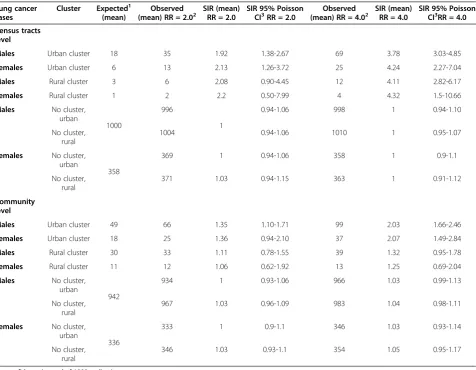
The results of the eight (2 cluster types × 2 risk magni-tudes × 2 gender groups) times 1 000 risk realizations are displayed in Table 1 which contains the mean of the expected counts based on the background incidence, the observed sampled counts based on the artificial risk

Table 1 Summary results of 1000 realizations from an inhomogeneous Poisson process

Lung cancer cases

Cluster Expected1 (mean)

Observed (mean) RR = 2.02

SIR (mean) RR = 2.0

SIR 95% Poisson CI3RR = 2.0

Observed (mean) RR = 4.02

SIR (mean) RR = 4.0

SIR 95% Poisson CI3RR = 4.0

Census tracts level

Males Urban cluster 18 35 1.92 1.38-2.67 69 3.78 3.03-4.85

Females Urban cluster 6 13 2.13 1.26-3.72 25 4.24 2.27-7.04

Males Rural cluster 3 6 2.08 0.90-4.45 12 4.11 2.82-6.17

Females Rural cluster 1 2 2.2 0.50-7.99 4 4.32 1.5-10.66

Males No cluster, urban

1000

996

1

0.94-1.06 998 1 0.94-1.10

No cluster, rural

1004 0.94-1.06 1010 1 0.95-1.07

Females No cluster, urban

358

369 1 0.94-1.06 358 1 0.9-1.1

No cluster, rural

371 1.03 0.94-1.15 363 1 0.91-1.12

Community level

Males Urban cluster 49 66 1.35 1.10-1.71 99 2.03 1.66-2.46

Females Urban cluster 18 25 1.36 0.94-2.10 37 2.07 1.49-2.84

Males Rural cluster 30 33 1.11 0.78-1.55 39 1.32 0.95-1.78

Females Rural cluster 11 12 1.06 0.62-1.92 13 1.25 0.69-2.04

Males No cluster, urban

942

934 1 0.93-1.06 966 1.03 0.99-1.13

No cluster, rural

967 1.03 0.96-1.09 983 1.04 0.98-1.11

Females No cluster, urban

336

333 1 0.9-1.1 346 1.03 0.93-1.14

No cluster, rural

346 1.03 0.93-1.1 354 1.05 0.95-1.17

CI = confidence interval of 1000 realizations.

1

Expected under the null hypothesis (= background incidence).

2

Observed with sampling using an inhomogeneous Poisson process.

3

Boice-Monson Method.

(8)

surface, and the simulated relative risk increases (expressed as SIR). On the census tract scale, an ef-fective realization of the two-and four-fold risk in-creases was achieved on average for the urban and rural clusters in men and women. However, the 95% Poisson CIs were much narrower in the urban clus-ters while they clearly included the null value for a RR1= 2.0 in the rural clusters. The mean SIR values for

the non-cluster areas were 1.0 with a narrow 95% CI. On the community scale, the SIR values were much more weakly elevated: the point estimates ranged from 1.06 to 1.35 with RR1= 2.0 and from 1.25 to 2.07 for a RR2= 4.0.

At this scale, only the urban clusters with a simulated RR2= 4.0 and the male urban cluster for RR1 = 2.0

showed 95% CIs for the SIR that did not include the null value. On the other hand, the CIs were wide in the rural clusters and they included mostly the null value. The aver-age SIR was 1.0 in the non-cluster areas with narrow CIs.

Results of the local cluster tests

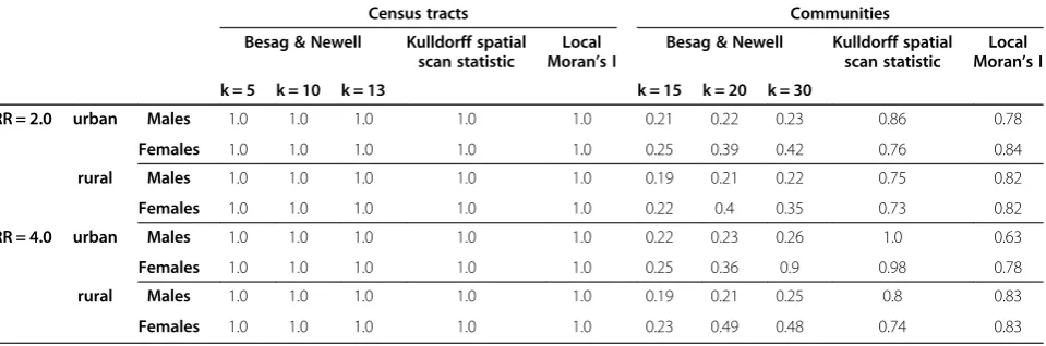
The statistical power of the Kulldorff spatial scan statis-tic, the approach of Besag & Newell (BN) and local Mor-an’s I (LMI) is given in Table 2. The results show at the census tract scale that all tests have a sufficient power (100%) to detect clustering under the eight risk (data-set) combinations. At community scale the power is gen-erally decreased, but while the Kulldorff spatial scan statistic and the LMI still had statistical power (>63%) to detect clustering, the BN method showed a considerable loss in power. In fact, only the female urban cluster realization with a four-fold risk increase could be identi-fied with 90% power for 30 enclosed cases (k = 30).

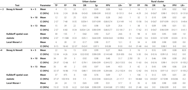
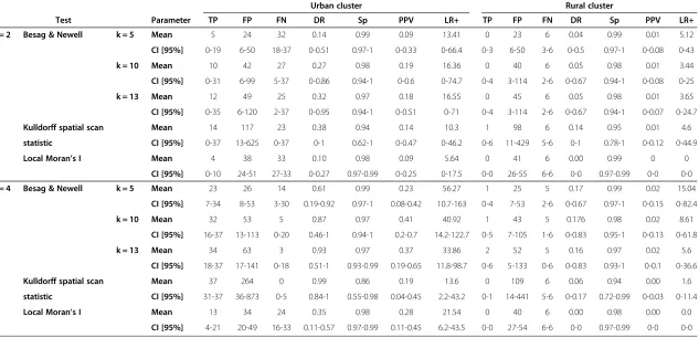
The accuracy of the cluster locations at census tract level using the eight different model realizations are dis-played in Table 3 for male and in Table 4 for female lung cancer cases. All local cluster tests showed a very high

specificity reflecting the large number of non-cluster areas. For all local cluster tests there is an increase in the mean detection rate (DR) with increasing risk mag-nitudes in the cluster areas. The increase of the mean DR is especially distinct in the urban cluster. Kulldorff spatial scan statistic had the highest detection rate in the urban cluster regardless of the risk magnitude but it also produced the highest number of false positives which re-sulted in low values for PPV and LR+. With a cluster RR1= 2.0, the Besag & Newell test for the urban cluster

had only mean DRs lower than 0.5 while the positive predictive power (PPV) was in the range of Kulldorff spatial scan statistic for that risk. With cluster RR2= 4.0,

the mean DR for the BN rose above 0.9 with PPVs be-tween 0.27 and 0.48, whereas Kulldorff spatial scan stat-istic had only a mean PPV 0.09. The local Moran’s I showed the weakest ability of all applied local cluster tests to detect and predict clusters with RR1= 2.0 but it

had the highest mean PPV (0.51) for the urban clusters of lung cancer in males when RR2= 4.0. Further, it was

the only method where the mean DR increased with simultaneously decreasing of FPs when the RR was higher. However, the test accuracy in women was gener-ally lower than in men. Of note, in the rural clusters of lung cancer, the DR, PPV and LR + were all consistently very low, both in men and women and regardless of the risk magnitude.

At the community level, a high number of non-cluster communities (n = 76) was compared in each dataset combination to only one community that harboured the cluster areas in its borders (Table 5). Generally, however, the same pattern can be observed as at census tract level: The urban clusters are better detected than the rural ones and the clusters were better detected in the male population than in the female. The overall DR for the Kulldorff spatial scan statistic and LMI increased

Table 2 Power of the Kulldorff spatial scan statistic, the Besag & Newell statistic, and the local Moran’s I statistic for detecting spatial clustering

Census tracts Communities

Besag & Newell Kulldorff spatial scan statistic

Local Moran’s I

Besag & Newell Kulldorff spatial scan statistic

Local Moran’s I

k = 5 k = 10 k = 13 k = 15 k = 20 k = 30

RR = 2.0 urban Males 1.0 1.0 1.0 1.0 1.0 0.21 0.22 0.23 0.86 0.78

Females 1.0 1.0 1.0 1.0 1.0 0.25 0.39 0.42 0.76 0.84

rural Males 1.0 1.0 1.0 1.0 1.0 0.19 0.21 0.22 0.75 0.82

Females 1.0 1.0 1.0 1.0 1.0 0.22 0.4 0.35 0.73 0.82

RR = 4.0 urban Males 1.0 1.0 1.0 1.0 1.0 0.22 0.23 0.26 1.0 0.63

Females 1.0 1.0 1.0 1.0 1.0 0.25 0.36 0.9 0.98 0.78

rural Males 1.0 1.0 1.0 1.0 1.0 0.19 0.21 0.25 0.8 0.83

(9)

Table 3 Summary of the local cluster test results for male lung cancer for both risk magnitudes, by census tract level

Urban cluster Rural cluster

Test Parameter TP FP FN DR Sp PPV LR+ TP FP FN DR Sp PPV LR+

RR = 2 Besag & Newell k = 5 Mean 4 15 33 0.11 0.99 0.08 16.6 1 16 5 0.11 0.99 0.02 18.0

CI [95%] 0-16 2-24 20-36 0-0.43 0.98-0.99 0-0.32 0-131.5 0-4 4-29 2-6 0-0.67 0.98-1 0-0.13 0-131.8

k = 10 Mean 12 32 25 0.33 0.98 0.28 24.0 1 32 5 0.10 0.98 0.02 6.8

CI [95%] 2-37 7-48 0-35 0.054-1 0.97-0.99 0.06-0.74 3.3-149 1-0 15-58 5-6 0-0.67 0.97-0.99 0-0.13 0-49.4

k = 13 Mean 15 39 22 0.41 0.98 0.29 25.4 1 38 5 0.09 0.98 0.01 5.5

CI [95%] 2-37 6-60 0-34 0.054-1.24 0.96-0.99 0.06-0.77 3.5-181.7 3-1 17-62 3-5 0-0.67 0.96-0.99 0-0.11 0-41.1

Kulldorff spatial scan Mean 30 135 7 0.82 0.93 0.27 24.6 0 98 6 0.03 0.95 0.00 1.0

statistic CI [95%] 2-37 11-588 0-33 0.05-1 0.64-0.99 0.034-0.63 1.8-90.6 0-1 14-425 5-6 0-0.03 0.7-0.99 0-0.03 0-1.5

Local Moran’s I Mean 6 30 31 0.17 0.98 0.17 12.1 0 34 6 0.00 0.98 0.00 0.0

CI [95%] 0-15 18-43 22-37 0-0.41 0.97-1 0-0.38 0-33 0-0 21-48 6-6 0-0 0.98-1 0-0 0-0

RR=4 Besag & Newell k = 5 Mean 22 16 15 0.59 0.99 0.27 86.6 3 16 3 0.55 0.99 0.08 82.0

CI [95%] 12-34 4-26 3-24 0.32-0.92 0.98-0.99 0.14-0.48 35.9-305 0-6 5-30 0-6 0-0.16 0.99-1.0 0-0.2 0-0

k = 10 Mean 34 39 3 0.92 0.98 0.48 51.7 2.781 35 3 0.46 0.98 0.08 29.2

CI [95%] 29-37 12-66 0-7 0.78-1 0.96-0.99 0.34-0.72 26.3-133.5 0-6 11-63 0-6 0-0.16 0.98-1 0-0.19 0-105.2

k = 13 Mean 35 49 2 0.95 0.97 0.44 43.3 3 42 3 0.43 0.98 0.06 22.8

CI [95%] 32-37 16-86 7-10 0.86-1 0.95-0.99 0.28-0.66 21.2-102.4 0-6 12-82 0-6 0-0.16 0.97-1.0 0-0.17 0-105.2

statistic CI [95%] 37-37 103-914 0-0 1-1 0.53-0.94 0.04-0.25 2.1-17.7 0-1 18-460 5-6 0-0.027 0.7-0.98 0-0.036 0-2

Local Moran I Mean 24 24 13 0.65 0.99 0.51 57.7 0 35 6 0.00 0.98 0.00 0.0

CI [95%] 15-31 13-35 6-22 0.41-0.84 0.98-0.99 0.34-0.68 27.1-109.2 0-0 21-48 6-6 0-0 0.96-0.99 0-0 0-0

Lemke

et

al.

Internationa

lJournal

of

Health

Geograp

hics

2013,

12

:54

Page

9

o

f

1

8

http://ww

w.ij-healthgeo

graphics.co

m/content/12/1

(10)

Table 4 Summary of the local cluster test results for female lung cancer for both risk magnitudes, by census tract level

Urban cluster Rural cluster

Test Parameter TP FP FN DR Sp PPV LR+ TP FP FN DR Sp PPV LR+

CI [95%] 0-19 6-50 18-37 0-0.51 0.97-1 0-0.33 0-66.4 0-3 6-50 3-6 0-0.5 0.97-1 0-0.08 0-43

k = 10 Mean 10 42 27 0.27 0.98 0.19 16.36 0 40 6 0.05 0.98 0.01 3.44

CI [95%] 0-31 6-99 5-37 0-0.86 0.94-1 0-0.6 0-74.7 0-4 3-114 2-6 0-0.67 0.94-1 0-0.08 0-25

k = 13 Mean 12 49 25 0.32 0.97 0.18 16.55 0 45 6 0.05 0.98 0.01 3.65

CI [95%] 0-35 6-120 2-37 0-0.95 0.94-1 0-0.51 0-71 0-4 3-114 2-6 0-0.67 0.94-1 0-0.07 0-24.7

statistic CI [95%] 0-37 13-625 0-37 0-1 0.62-1 0-0.47 0-46.2 0-6 11-429 5-6 0-1 0.78-1 0-0.12 0-44.9

Local Moran’s I Mean 4 38 33 0.10 0.98 0.09 5.64 0 41 6 0.00 0.99 0 0

CI [95%] 0-10 24-51 27-33 0-0.27 0.97-0.99 0-0.25 0-17.5 0-0 26-55 6-6 0-0 0.97-0.99 0-0 0-0

CI [95%] 7-34 8-53 3-30 0.19-0.92 0.97-1 0.08-0.42 10.7-163 0-4 7-53 2-6 0-0.67 0.97-1 0-0.15 0-82.4

k = 10 Mean 32 53 5 0.87 0.97 0.41 40.92 1 43 5 0.176 0.98 0.02 8.61

CI [95%] 16-37 13-113 0-20 0.46-1 0.94-1 0.2-0.7 14.2-122.7 0-5 7-105 1-6 0-0.83 0.95-1 0-0.13 0-61.8

k = 13 Mean 34 63 3 0.93 0.97 0.37 33.86 2 52 5 0.16 0.97 0.02 5.6

CI [95%] 18-37 17-141 0-18 0.51-1 0.93-0.99 0.19-0.65 11.8-98.7 0-6 5-133 0-6 0-0.83 0.93-1 0-0.1 0-36.6

statistic CI [95%] 31-37 36-873 0-5 0.84-1 0.55-0.98 0.04-0.45 2.2-43.2 0-1 14-441 5-6 0-0.17 0.72-0.99 0-0.03 0-11.4

Local Moran’s I Mean 13 34 24 0.35 0.98 0.28 21.54 0 40 6 0.00 0.98 0.00 0.0

CI [95%] 4-21 20-49 16-33 0.11-0.57 0.97-0.99 0.11-0.45 6.2-43.5 0-0 27-54 6-6 0-0 0.97-0.99 0-0 0-0

Internationa

lJournal

of

Health

Geograp

hics

2013,

12

:54

Page

10

of

18

graphics.co

m/content/12/1

(11)

Table 5 Summary of the results for male and female lung cancer, by community level

Male lung cancers Female lung cancers

RR Method Parameter TP urban FP urban TP rural FP rural TP urban FP urban TP rural FP rural

RR = 2.0 Besag & k = 15 sum 210 80 1 269 27 17 1 361

Newell DR 0.21 0.00 0.03 0.00

PPV 0.72 0.00 0.61 0.00

LR+ 202.13 135.9 0.00

k = 20 sum 220 40 240 92 39 51 414 384

DR 0.22 0.24 0.04 0.41

PPV 0.85 0.72 0.43 0.52

LR+ 423.50 200.87 60.4 69.45

k = 30 sum 220 150 1 361 50 57 1 842

DR 0.22 0.00 0.05 0.00

PPV 0.59 0.00 0.47 0.00

LR+ 112.93 0.00 67.5 0.00

Kulldorff sum 501 3974 92 3770 744 3220 80 3996

spatial scan DR 0.50 0.09 0.74 0.08

statistic PPV 0.11 0.02 0.19 0.02

LR+ 9.71 1.88 17.7 1.54

Local sum 190 1512 37 1728 34 126 52 1569

Moran’s I DR 0.19 0.04 0.03 0.05

exact PPV 0.11 0.02 0.21 0.03

LR+ 9.68 1.65 20.78 2.55

RR = 4.0 Besag & k = 15 sum 126 172 2 260 242 130 1 368

Newell DR 0.13 0.00 0.24 0.00

PPV 0.42 0.01 0.65 0.00

LR+ 56.41 0.59 143.34 0.00

k = 20 sum 232 102 224 120 384 382 464 610

DR 0.23 0.22 0.38 0.46

PPV 0.69 0.65 0.50 0.43

LR+ 175.14 143.73 77.40 58.57

k = 30 sum 250 80 2 321 920 810 2 1105

DR 0.25 0.00 0.92 0.00

PPV 0.76 0.01 0.53 0.00

LR+ 240.63 0.48 87.46 0.00

Kulldorff’s sum 999 11542 351 5590 916 6506 155 4469

spatial scan DR 1.00 0.35 0.92 0.16

statistic PPV 0.08 0.06 0.12 0.03

LR+ 6.66 4.83 10.84 2.67

Local sum 398 732 106 1636 304 1130 72 1588

Moran’s I DR 0.40 0.11 0.30 0.07

exact PPV 0.35 0.06 0.21 0.04

LR+ 41.87 4.99 20.72 3.49

TP = true positive, FP = false positive; DR = detection rate, PPV = positive predictive value. LR + = likelihood ratio of a positive test result.

(12)

with higher simulated cluster RR and the Kulldorff spatial scan statistic had the highest DRs, but at the cost of an immense number of FPs. The DRs using the BN test were similar for the two cluster RR magnitudes but the FPs were higher when the RR was higher. Only the LMI showed that increases of the DR were accompanied by remarkable FP decreases.

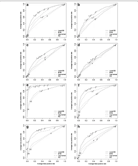
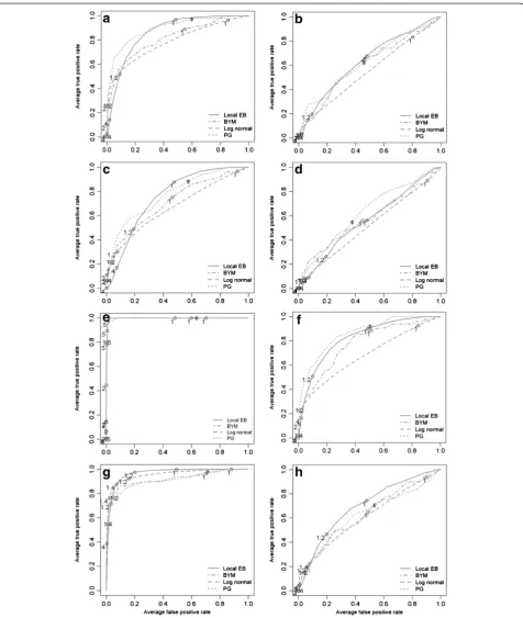
Results of the Bayesian smoothing methods

The results of the Bayesian smoothing techniques are summarized using ROC curves in Figure 4 (census tracts) and Figure 5 (communities). Across all cluster types and cluster risk magnitudes, the methods that im-plement a spatial neighbourhood, and therefore smooth the risk estimate towards a local mean, performed better than the global methods. At census tract scale and with a cluster RR1= 2.0, the local EB method had the highest

mean DR (between 0.6 and 0.7) with the lowest average FP rate at a threshold of 1.4 in the urban clusters. For the rural cluster the threshold was the same but the mean DR was lower (0.5-0.6) with a higher mean FPR. In the female population, the ROC curves are close to the diagonal line, denoting that the methods have only a minor (urban cluster) or no (rural cluster) discrimin-atory power. With increasing cluster risk magnitude the test accuracy for all methods was improved, that is, the area under the curve (AUC) was augmented. For the urban cluster in men (Figure 4e), the BYM model showed a slightly better performance than the local EB: the BYM model achieved its highest mean DR (>0.8) with a minimum FPR (<0.05) at threshold values between 1.2 and 1.4 while the local EB had at compar-able threshold values a higher FPR (>0.2). For the urban cluster in women (Figure 4g), the same pattern was observed: For same risk threshold of 1.2 the local EB model had a higher DR (>0.8) but with a higher mean FPR (>0.20), while the BYM model had a lower mean DR (≈0.5) but with a lower FPR (<0.05).

In general, similar patterns were observed at the com-munity level. The local EB achieved the highest accuracy among all smoothing methods and test accuracy in-creased with increasing cluster risk magnitude. However, for RR1= 2.0, the mean DR were lower and the mean

FPR higher as at census tract level. With increasing cluster RR magnitude the mean DR for the urban clus-ters (Figure 5e and f ) increased to almost 1.0 with a mean FP <0.05 at thresholds between 1.2 and 1.4.

Discussion

The aim of this simulation study was to evaluate differ-ent methods in their ability to iddiffer-entify spatial clusters of lung cancer using real-life data from an epidemio-logical cancer registry in Germany. Little is known about the performance of local cluster tests and

Bayesian smoothing methods under conditions that differ by relative risks and spatial scale, that is, small and large population sizes and the respective data ag-gregations. We found that the local Bayesian smooth-ing models (local EB and BYM) generally had a better test accuracy than the global models. However, at census tract level and for a RR = 2.0, the local clusters tests gener-ally showed lower FPRs than the Bayesian smoothing methods but with comparable DRs. Also when increasing the cluster RR magnitude, the local cluster tests had lower FPRs with comparable the DRs. Only at the community level and for a four-fold risk magnitude this pattern was reversed: with comparable DR the smoothing models had lower FPRs.

We implemented a simulation process with eight dif-ferent conditions under which the method performance was evaluated. The conditions encompassed the compar-isons of two magnitudes of cluster risk elevations (RR1=

2.0 and RR2= 4.0), of small scale (census tracts) and

(13)

Figure 4Averaged ROC curves of the four applied Bayesian smoothing models at census tract level.The letter indicating the different risk realizations:(a)urban cluster in the male population (RR = 2.0);(b)rural cluster the male population (RR = 2.0);(c)urban cluster in the female population (RR = 2.0);(d)rural cluster the male population (RR = 2.0);(e)urban cluster in the male population (RR = 4.0);(f)rural cluster in the male population (RR = 4.0); and(g)rural cluster in the female population (RR = 4.0).

(14)

(15)

Local cluster tests

At census tract level, all cluster tests showed a power of 100% for the eight simulation scenarios, probably because the risk was realized in a sufficient manner. The statistical power is primarily influenced by two factors: the sample size and the true difference between the null and alterna-tive hypothesis [34]. Therefore, the subsequent analysis of the location accuracy of the tests is not affected by low power. By contrast, on the community level a decrease in power was observed that was most likely due to the dilu-tion of the realized risk as a consequence of data aggrega-tion and the different samples sizes (male vs female population, urban versus rural population density). The fact, that the LMI showed the lowest power for the most favourable cluster scenario, e.g. highest risk realization und highest sample size (urban cluster in male & fe-male population with a RR2= 4.0) was probably due to

a less production of false positive locations than in the other cluster scenarios. In addition, it became also ap-parent that the power of the BN method is very sensi-tive to the choice of k. Regarding the accuracy of location, Kulldorff’s spatial scan statistic had the great-est ability among the local cluster tgreat-ests to correctly identify lung cancer clusters in urban as well as rural environments; this was particularly true at the census tract level. However, the predictive power, that is, the probability that a positive test result correctly repre-sented a cluster, was at the same time low due to the high numbers of FPs. These results are consistent with the findings of Aamondt et al. [35] who applied a com-parable simulation design in order to evaluate the sensitivity and specificity of three local cluster tests (Kulldorff spatial scan statistic, BYM, GAM) in Norwegian municipalities (comparable in area and population sizes to German communities). They found an average detection rate for urban clusters of 75% when simulating a risk in-crease of 50% (RR = 1.5) and of 80% for a RR = 4.0. For a comparable rural cluster they reported a detection rate of 51% (RR = 1.5) and of 87% (RR = 4), respectively. The higher DR values for the rural cluster in [35] were attribut-able to a larger sample size, that is, 1.1% of the total Norwegian population was included in this cluster. Unfortunately, Aamondt et al. [35] provide no infor-mation about the numbers of the FPs and therefore about the predictive abilities of the applied tests. Huang et al. [36] showed in their simulation study that Kulldorff’s spatial scan statistic achieved only a PPV of 0% for a RR of 1.2 for lung cancer in male and female with a sample size of 5000 cases. The poor predictive power of the Kulldorff spatial scan statistic has been noted before: areas with a low incidence rate (far below the global mean) can be included in the cluster area and the local average within this cluster remains suffi-ciently elevated [12,37]. The BN method is based on

the number of k enclosed disease cases which influ-ences greatly the power and therefore the detection rate and the predictive power of the test. At census tract level, the BN method had a mean DR for both risk magnitudes that was lower than that of Kulldorff’s spatial scan statistic for the k-threshold nearest to true number of enclosed cases. Nevertheless, the BN method had a slightly better predictive performance than Kull-dorff’s spatial scan statistic because it produced far less FPs. This, however, turns out to be particularly distinct for the urban cluster scenario in females for a RR2= 4.0 at

community level, where a power and DR of >90% were achieved with only minimal increased FPs as compared to the Kulldorff spatial scan statistic. But this was only ac-complished with the choice of k that was nearest to the true number of observed cases (k = 30).Costa & Assun-cao [38] reported in their comparison of the Kulldorff spatial scan statistic and the BN method that the methods perform similarly in urban settings with a sufficiently large background population but show major differences in sparsely populated areas. We observed this pattern in par-ticular in the female urban cluster but not for the male population because the k-threshold was far different from the true number of enclosed cases.

The LMI method level showed the weakest ability to identify clusters and had the lowest ability to predict the cluster correctly (compared to Kulldorff spatial scan stat-istic and the BN method for best k-threshold). These findings confirm previous simulation studies [8,11-13] which mentioned that LMI had the poorest performance of the local cluster tests. But for the urban cluster in males an interesting trend was observed: With increas-ing the risk it was the only local cluster test where the increases of TPs were accompanied by a decrease of FP. However, this could be only observed in the urban cluster realization in males, denoting that the applied version of LMI is sensitive to the small number problem. Therefore, it appears reasonable to include a modified version of the LMI in an R package that adjusts for heterogeneous popu-lation densities as proposed in [39]. At the community level only spatial outliers are detected, and the exact ver-sion of the test was applied because only few spatial neighbours exist which makes the normality assump-tion arguable. For a twofold elevated cluster risk, the risk realization in the community is too small to be de-tected as a spatial outlier unlike for a four-fold risk in-crease: here the LMI had a greater ability to detect the cluster community than the BN method.

Bayesian smoothing methods

The use of Bayesian smoothing methods for cluster de-tection are generally characterized by a decision whether the DR should be maximised or the FPR should be mini-mised for a specific RR cut-off that serves as threshold

(16)

value for defining a cluster. The results of the Bayesian models are discussed with the objective of evaluating the DR of each of the four models at a minimum FPR (or high specificity).

The global models (PG and log normal) showed poorer test accuracy than the local models and the differences be-tween these two global models were not very distinct. The global models have no definition of a spatial neighbour-hood and therefore the risk estimates were smoothed to-wards the global mean. This is expressed by the course of their ROC curves which were very close to the plot diag-onal implying very low test accuracy. This was particularly clear for cluster RR = 2.0, where all models failed to detect the rural cluster in females, possibly due to the low realized risk caused by small sample sizes and dilution effects in this cluster type. For the four-fold RR the test accuracy was augmented for all models, however, the global models were still less accurate than the local ones. Of note, the differ-ences were more distinct than for the two-fold RR realization, implying that the risk signal in the cluster areas were not oversmoothed but rather consolidated. This became particularly apparent in the male urban cluster where the test accuracy of the BYM model ex-ceed that of the local EB model (showing both higher DR together with a lower FPR). This describes also the situation where the BYM model was most powerful, namely moderate sized expected counts (>50) and/or high excess risk [40]. Only few simulation studies are available that compare Bayesian smoothing methods to local cluster tests. The results are consistent with the findings of Aamondt et al. [35] who found in a compar-able cluster setting a mean sensitivity between 0-1% for a relative risk of 1.5 but a sensitivity of 85-99% for a RR = 4.0. Similarly, Richardson et al. [40] reported that the BYM model is essentially conservative for moderate rela-tive risks (RR < 2.0) and they concluded that it is nearly impossible to detect localized risk areas if these are not based on a large (RR > 3.0) excess risk or, in the case of a moderate risk (RR > 2.0), on substantial numbers of ex-pected counts of approximately 50 or more. At commu-nity level, the expected counts are consolidated by data aggregation although it was noted that the rural cluster in females could neither be detected at RR = 2.0 nor at RR = 4.0, most likely because of the dilution effects in this clus-ter. The local EB had a mean DR for a RR = 2.0 that was comparable to that of Kulldorff’s spatial scan statistic al-though with a higher FPR. However, with a four-fold rela-tive risk in a cluster, all Bayesian models had the same higher test accuracy for the male urban cluster, denoting that the expected counts and the relative risk was realized in a sufficient manner This resulted in a performance that was better than that of the local cluster tests. This was also observed for the female urban cluster but the ROC curves were affected by the reduced sample size.

Strengths and limitations

There are strengths and limitations of this study. A major strength of this study is the modelling of real can-cer incidence data in small and large sample sizes with moderately to highly increased risks and at different spatial scales of data aggregation. Furthermore, the model-ling of the observed cases as Poisson distributed reflects a more meaningful assumption than a fixed sample size and it increases the applicability of the study results to realistic cancer cluster patterns. This study was limited in terms of the local cluster tests used. Dozens of local cluster tests exist [41-44] and it is possible that other tests may be more successful to detect and predict the clusters. How-ever, a main objective of this study was to apply well-known methods that are available in an open source environment. For creating a continuous risk surface on the basis of area data, Poisson kriging [45] may be used. This technique may result in less smoothing, however, to our knowledge the Poisson kriging approach is not yet properly implemented in an R-package. This ap-plies also to the use of the modified version of local Mor-an’s I as described in [38] that adjusts for heterogeneous population densities.

Summary and conclusion

In summary, this simulation study suggests that for the identification of geographic cancer clusters the use of a smaller spatial scale is generally preferable to a higher data aggregation scale. One reason is that cancer is a fairly rare disease and that cancer clusters tend to be limited in time and small in place. Data aggregation re-sults in diluted risks masking the existence of small high risk areas within a larger aggregate of many average risk areas; this impedes the detection of small cancer clusters with a moderate, and even high, risk increase. This is not balanced out by the higher numerical precision ob-tained by using larger aggregates. With regard to the tests applied, the local cluster tests seem preferable to the smoothing methods for clusters with a moderate risk increase at both spatial scales. Only with very high clus-ter risks, the local Bayesian smoothing models have lower FPRs for comparable DRs on the aggregate spatial level (community level). It should be noted that, despite the high DR, the Kulldorff spatial scan statistic had a very low predictive ability whereas, by contrast, the BN method showed a good test accuracy but was extremely sensitive to the right choice of the k threshold. Further, the LMI method is expected to probably show a better performance when adjustments for the heterogeneous background populations can be achieved. For the smooth-ing methods, the study suggests that the local models are generally preferable to the global models.

(17)

Smaller scales have to be preferred to enhance more effective cluster detections. We suggest a two-stage ap-proach that combines highly sensitive methods as a first-line screening with methods of higher predictive ability in order to reduce the number of false positive results. For small-scaled data the results of the Kull-dorff spatial scan statistic pre-screening could be used to refine the parameter k and then the BN methods ap-pears suitable to re-evaluate the identified clusters. When using a higher data aggregation level, the local EB model appears more suitable. Future research into cancer cluster detection should focus on the numerical and statistical stabilization of the risk measures. Thus, it should be quantitatively evaluated which cancer entities are actually appropriate for a prospective cluster monitor-ing or whether, in cases of low incidence rates with too low count numbers, cluster monitoring should not be en-couraged. In addition, the reduction of risk measure vari-ability needs to be emphasized in sparsely populated areas. Apart from spatial aggregation (only to a degree that avoids too much loss of the risk signal), temporal ag-gregation, especially in the female population and for rare tumours, should be considered to help stabilize the risk measures.

Competing interests

The authors declare that they have no competing interests.

Authors_’contributions

DL and HWH planned and designed the study, VM and OH provided the cancer registry data; DL programmed the R-code, administered the simulations, analysed the data and wrote the first manuscript draft, HWH and EP reviewed the manuscript and provided guidance on all issues related to epidemiological and spatial statistical side of the analysis. All authors contributed to the intellectual content and approved the final manuscript.

Acknowledgement

We acknowledge support by Open Access Publication Fund of University of Münster.

Author details

1_{Institute of Epidemiology and Social Medicine, Medical Faculty, Westfälische} Wilhelms-Universität Münster, Albert-Schweitzer-Campus 1 D3, D 48149, Münster, Germany.2_{Institute for Geoinformatics, Geosciences Faculty,} Westfälische Wilhelms Universität Münster, Münster, Germany.

3_{Epidemiological Cancer Registry North Rhine-Westphalia, Münster, Germany.}

Received: 16 August 2013 Accepted: 1 December 2013 Published: 7 December 2013

References

1. Monitoring in epidemiologischen Krebsregistern: Möglichkeiten–Grenzen– Risiken.http://www.krebsregister-niedersachsen.de/registerstelle/?page_id=2071. 2. Kieschke J:Auswertung des EKN zur Krebshäufigkeit in der

Samtgemeinde Asse. InEKN-Bericht.Edited by Epidemiologisches Krebsregister Niedersachsen. Oldenburg, Germany; 2010.

3. Dreesmann J:Statistische Erkennung Räumlicher Cluster- Erfahrungen aus der Infektionsepidemiologie. InMonitoring-Workshop.Edited by Niedersächsisches Landesgesundheitsamt. Oldenburg, Germany; 2012. 4. Olsen SF, Martuzzi M, Elliott P:Cluster analysis and disease mapping–why,

when, and how? A step by step guide.BMJ1996,313(7061):863–866. 5. Waller LA, Gotway CA:Applied Spatial Statistics for Public Health Data.

Hoboken, N.J.: John Wiley & Sons; 2004.

6. Rothman KJ:A Sobering Start for the Cluster busters’Conference.

Am J Epidemiol1990,132(1 Suppl):S6–S13.

7. Goodman M, Naiman JS, Goodman D, LaKind JS:Cancer clusters in the USA: what do the last twenty years of state and federal investigations tell us?Crit Rev Toxicol2012,42(6):474_–490.

8. Song C, Kulldorff M:Power evaluation of disease clustering tests.

Int J Health Geogr2003,2(1):9.

9. Schmiedel S, Blettner M, Schuz J:Statistical power of disease cluster and clustering tests for rare diseases: a simulation study of point sources.

Spat Spatiotemporal Epidemiol2012,3(3):235–242.

10. Ozonoff A, Jeffery C, Manjourides J, White LF, Pagano M:Effect of spatial resolution on cluster detection: a simulation study.Int J Health Geogr

2007,6:52.

11. Kulldorff M, Tango T, Park PJ:Power comparisons for disease clustering tests.Comput Stat Data An2003,42(4):665–684.

12. Jacquez GM:Cluster morphology analysis.Spat Spatiotemporal Epidemiol

2009,1(1):19–29.

13. Jackson MC, Huang L, Luo J, Hachey M, Feuer E:Comparison of tests for spatial heterogeneity on data with global clustering patterns and outliers.Int J Health Geogr2009,8:55.

14. Assuncao RM, Reis EA:A new proposal to adjust Moran_’s I for population density.Stat Med1999,18(16):2147–2162.

15. Gregorio DI, Dechello LM, Samociuk H, Kulldorff M:Lumping or splitting: seeking the preferred areal unit for health geography studies.Int J Health Geogr2005,4(1):6.

16. Amtliche Statistik (NRW).http://www.it.nrw.de/statistik/. 17. INFAS Geodata.http://www.infas-geodaten.de/.

18. Epidemiologisches Krebsregister (NRW).Interaktive Datenabfrage. http:// www.krebsregister.nrw.de/index.php?id=113/.

19. Pfeiffer D:Spatial Analysis in Epidemiology. Oxford.New York: Oxford University Press; 2008.

20. Gómez-Rubio V, Ferrándiz-Ferragud J, López-Quílez A:Detecting clusters of disease with R.J Geogr Syst2005,7(2):189–206.

21. Spdep.http://cran.r-project.org/web/packages/spdep/index.html. 22. R version (2.13.1).http://cran.r-project.org/bin/windows/base/old/2.13.1/. 23. Bivand R:Spatial statistics: geospatial information modeling and

thematic mapping.Environ Plann B2013,40(1):189–189.

24. Bivand R:Applying measures of spatial autocorrelation: computation and simulation.Geogr Anal2009,41(4):375_–384.

25. Benjamini Y, Hochberg Y:Controlling the false discovery rate - a practical and powerful approach to multiple testing.J Roy Stat Soc B Met1995, 57(1):289–300.

26. de Castro MC, Singer BH:Controlling the false discovery rate: a new application to account for multiple and dependent tests in local statistics of spatial association.Geogr Anal2006,38(2):180–208. 27. Kulldorff M:A spatial scan statistic.Commun Stat-Theor M1997,

26(6):1481_–1496.

28. Besag J, Newell J:The detection of clusters in rare diseases.J Roy Stat Soc a Sta1991,154:143–155.

29. R Development Core Team:R: Language and Environment for Statistical Computing.Vienna, Austria: R Foundation for Statistical Computing; 2013. 30. Clayton D, Kaldor J:Empirical bayes estimates of age-standardized

relative risks for use in disease mapping.Biometrics1987, 43(3):671–681.

31. Bivand RS, Pebesma EJ, GomezRubio V:Applied Spatial Data Analysis with R.2008.

32. Besag J, York J, Mollie A:Bayesian image-restoration, with 2 applications in spatial statistics.Ann I Stat Math1991,43(1):1–20.

33. Lunn DJ, Thomas A, Best N, Spiegelhalter D:WinBUGS - a bayesian modelling framework: concepts, structure, and extensibility.

Stat Comput2000,10(4):325–337.

34. Waller LA, Hill EG, Rudd RA:The geography of power: Statistical performance of tests of clusters and clustering in heterogeneous populations.Stat Med2006,25(5):853–865.

35. Aamodt G, Samuelsen SO, Skrondal A:A simulation study of three methods for detecting disease clusters.Int J Health Geogr2006,5:15. 36. Huang L, Pickle LW, Das B:Evaluating spatial methods for investigating

global clustering and cluster detection of cancer cases.Stat Med2008, 27(25):5111–5142.

37. Tango T, Takahashi K:A flexibly shaped spatial scan statistic for detecting clusters.Int J Health Geogr2005,4:11.

(18)

38. Costa MA, Assunção RM:A fair comparison between the spatial scan and the BesagNewell disease clustering tests.Environ Ecol Stat Environmental and Ecological Statistics2005,12(3):301–319.

39. Jackson MC, Huang L, Xie QA, Tiwari RC:A modified version of Moran’s I.

Int J Health Geogr2010,9:33.

40. Richardson S, Thomson A, Best N, Elliott P:Interpreting posterior relative risk estimates in disease-mapping studies.Environ Health Persp2004, 112(9):1016–1025.

41. Lawson AB, Kulldorff M:A Review of Cluster Detection Methods. InDisease Mapping and Risk Assessment for Public Health.Edited by Lawson AB. New York: Wiley; 1999.

42. Kulldorff M, Song CH, Gregorio D, Samociuk H, DeChello L:Cancer map patterns - Are they random or not?Am J Prev Med2006,30(2):S37–S49. 43. Jacquez GM, Waller LA, Grimson R, Wartenberg D:The analysis of disease

clusters, part I: state of the art.Infect Control Hosp Epidemiol1996, 17(5):319–327.

44. Jacquez GM, Grimson R, Waller LA, Wartenberg D:The analysis of disease clusters, part II: introduction to techniques.Infect Control Hosp Epidemiol

1996,17(6):385–397.

45. Goovaerts P:Geostatistical analysis of disease data: accounting for spatial support and population density in the isopleth mapping of cancer mortality risk using area-to-point poisson kriging.Int J Health Geogr2006, 5:52.

doi:10.1186/1476-072X-12-54

Cite this article as:Lemkeet al.:Detecting cancer clusters in a regional population with local cluster tests and Bayesian smoothing methods: a

simulation study.International Journal of Health Geographics201312:54.

Submit your next manuscript to BioMed Central and take full advantage of:

• Convenient online submission

• Thorough peer review

• No space constraints or color ﬁgure charges

• Immediate publication on acceptance

• Inclusion in PubMed, CAS, Scopus and Google Scholar

• Research which is freely available for redistribution