Gianluca Antonacci
Faculty of Engineering, University of Trento Year: 2004
Supervisor: Prof. Marco Tubino
Università degli Studi di Trento Trento, Italy
The author wishes to thank Marco Tubino for rare but illuminating suggestions about the interpretation of data and providing valuable comments. Discussion with Dino Zardi was of great help to the author in focusing on the problem, especially from the meteorological point of view. Special thanks to Marco Ragazzi for useful suggestions and to Massimiliano de Franceschi for providing data acquired with the sonic anemometer
This work has been partly supported by the Environmental Protection Agency (APPA) of Bolzano and Trento, which have provided meteorological data used for testing the pro-posed conceptual tools.
I. Dispersion in valleys 3
1. Introduction to atmospheric physics 4
1.1. Dynamics in the atmospheric boundary layer . . . 4
1.1.1. Time and space scales . . . 4
1.1.2. The daily cycle of the atmospheric boundary layer . . . 5
1.1.3. Meteorological modelling. . . 6
1.2. Atmospheric stability . . . 7
1.2.1. Stability functions in the surface layer . . . 8
1.2.2. Stability over the entire ABL . . . 11
1.3. Air pollution modelling. . . 11
1.3.1. Mathematical formulation . . . 11
1.3.2. Lagrangian and Eulerian timescale . . . 12
1.3.3. Phenomenology . . . 13
1.4. Eddy diffusivity . . . 14
1.4.1. Estimate of eddy diffusivity in the surface layer . . . 14
1.4.2. Extension to the atmospheric boundary layer . . . 15
1.4.2.1. Non-local transport . . . 15
1.4.2.2. Unstable boundary layer . . . 16
1.4.2.3. Power law form. . . 16
2. Computing eddy diffusivity in valleys 18 2.1. The global approach . . . 18
2.1.1. Day time . . . 21
2.1.1.1. Geometric considerations . . . 22
2.1.2. Night-time . . . 29
2.2. The local approach . . . 30
2.2.1. Introduction. . . 30
2.2.2. Formulation of the model . . . 33
2.2.2.1. The solar path . . . 33
2.2.2.2. Shadow and sky view factor . . . 34
2.2.2.3. Global radiation . . . 35
2.2.2.4. Sensible heat flux . . . 37
2.2.2.5. Turbulent diffusivity . . . 38
2.2.3. Results . . . 39
2.2.4. Testing the model . . . 42
2.3. Conclusions . . . 45
3. Lagrangian modelling 47 3.1. The lagrangian approach . . . 47
3.1.1. Introduction. . . 47
3.1.2. Theory. . . 48
3.1.3. Extent of the puff . . . 49
3.1.4. Empirical formulation for TL andKz . . . 50
3.2. Langevin equation . . . 52
3.2.1. 2-equations model . . . 53
3.2.2. Gaussian turbulence . . . 54
3.2.3. Ito’s formula . . . 56
3.2.4. Difference between 1- and 2- equation models . . . 58
3.2.5. Kinematic interpretation of TL . . . 58
3.2.6. Skewed turbulence . . . 60
3.2.7. Buoyant plume rise . . . 63
3.3. Kernel method . . . 64
4. A 3D lagrangian model for non uniform terrain 70 4.1. Formulation . . . 70
4.1.1. Flow field . . . 70
4.1.2. Turbulence parametrization and lagrangian time scale . . . 73
4.1.3. Operational parameters . . . 74
4.3.1. Results . . . 78
4.3.2. Considerations on kernel method . . . 79
4.3.3. Comparison between CALPUFF and LAG3D . . . 82
4.3.4. Model limitations . . . 86
II. Dispersion in urban areas 88 5. Theoretical framework on traffic derived pollution 89 5.1. Introduction . . . 89
5.2. Characterization of urban climate . . . 90
5.2.1. Time and space scales in the urban environment . . . 90
5.2.2. The structure of the urban boundary layer . . . 91
5.2.3. Atmospheric stability in urban areas . . . 93
5.3. Flow field in urban areas . . . 93
5.3.1. Isolated buildings . . . 94
5.3.2. Groups of buildings. . . 98
5.3.3. Air flow in urban canyons . . . 99
5.3.4. Air flow along urban canyons . . . 101
5.3.5. Roughness height and displacement height . . . 102
5.4. Urban dispersion modelling . . . 105
5.4.1. Gaussian formulation. . . 106
5.5. Chemistry and deposition . . . 110
5.5.1. Deposition. . . 110
5.5.2. Chemistry and photochemical pollution . . . 113
5.5.2.1. Nitrogen oxides and ozone. . . 113
5.5.2.2. Airborne particulate . . . 114
6. Numerical modelling 119 6.1. The case of Trento . . . 119
6.2. Traffic flow and emission factors. . . 121
6.3. A 3D eulerian model . . . 124
6.3.1. Mathematical formulation . . . 126
6.3.2. Deposition. . . 129
6.4. 2D lagrangian model . . . 137
6.4.1. Formulation of the model . . . 137
6.4.1.1. Mean flow field . . . 138
6.4.1.2. Turbulence parametrization . . . 139
6.4.1.3. Lagrangian model . . . 141
6.4.2. Test simulation . . . 143
1.1. Daily evolution of the atmospheric boundary layer (Stull,1988). . . 6
1.2. The dimensionless functions ΦandΨ. . . 9
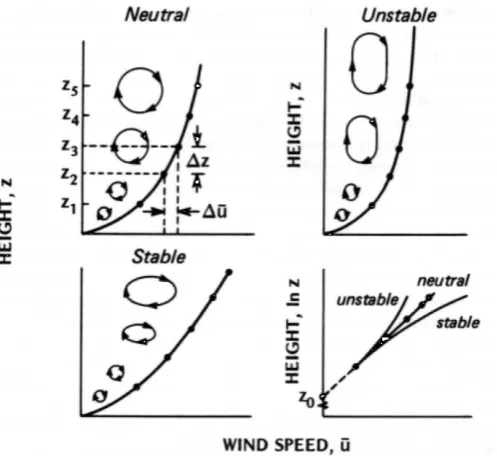
1.3. Wind profile modification due to stability (Thom,1975). . . 10
1.4. Behaviour of the effluent depending on the vertical temperature gradient; the dashed line represents the adiabatic temperature profile (adapted from Santomauro,1975). . . 14
2.1. Removal of the nocturnal stable layer (Whiteman, 1982). a) At sunrise the thermal inversion over the depth of the valley determines a situation of stable atmosphere; b) with the heating of the valley floor the growth of the CBL starts; c) the stable core sinks and upslope flows arise (secondary circulation); d) the well-mixed situation is reached around noon time. . . 19
2.2. Qualitative evolution of a) potential temperature and b) CBL and IT. . . . 20
2.3. Streamtubes scheme. . . 21
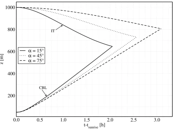
2.4. CBL growth and IT decrease with different valley floor widths andfc = 0.75. 24 2.5. CBL growth and IT decrease with different side slope inclination, fc = 0.75 and valley floor width L= 1000m. . . 24
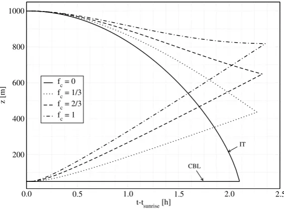
2.6. CBL growth and IT decrease with different energy partitioning coefficient, valley floor width L= 1000mand side slope inclination α= 30◦. . . 25
2.7. Time evolution of potential temperature vertical profile. . . 28
2.8. Time evolution of temperature vertical profile.. . . 29
2.9. Time evolution of eddy diffusivity vertical profile. . . 30
2.10. Study area and location of measurement and test points. . . 32
2.11. Sketch of the defined angles and notation. . . 34
and data registered by radiometers 1 and 2 (see figure 2.10). . . 39
2.14. Computed global solar radiation at different locations in a sunny day (see figure 2.10). . . 40
2.15. Computed values of sensible heat flux at different sites in the study area in a sunny day. . . 40
2.16. Measured values (at site 3) and computed values (at site 3, 4 and 5) of vertical turbulent diffusivity in the study area in a sunny day. . . 41
2.17. Comparison between computed and observed values of turbulent diffusivity at the test site 3 of the study area in a cloudy day. . . 41
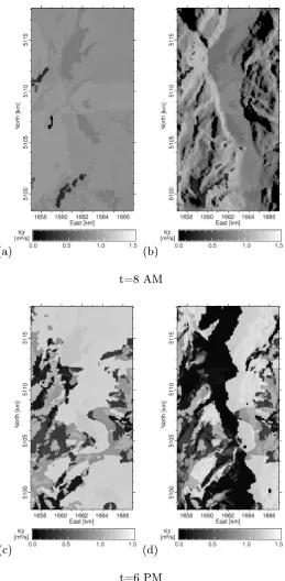
2.18. Maps of the computedKz at ground level (z= 3m) in the morning and in the late afternoon: (a, c) standard method; (b, d) present model. . . 43
2.19. Time lag of the model response with respect to field observations of the decay of turbulent diffusivity due to the extinction of direct radiation at sunset: a) winter and b) summer measurements. . . 44
2.20. Effluent smoke from domestic heating. The stable stratification maintains a compact plume (picture a) before sunrise, while the growing turbulence spreads it more rapidly (picture b), two hours after sunrise. Both pictures are taken at the same site in low wind condition. . . 44
2.21. Results of the numerical simulation, through the lagrangian model of chapter 3, of ground level emission, before sunrise, at site 5 under low wind condition: a) plan view and b) vertical section. Color scale is relative (red=maximum, blue=minimum concentration). Violet contour indicates irradiated surface, while black indicates not irradiate surface. . . 45
2.22. Results of the numerical simulation, through the lagrangian model of chapter 3, of ground level emission, two hours after sunrise, at site 5 under low wind condition: a) plan view and b) vertical section. Color scale is relative (red=maximum, blue=minimum concentration). Violet contour indicates irradiated surface, while black indicates not irradiate surface. . . 45
3.1. Lagrangian scheme: deterministic and stochastic motion. . . 48
3.2. Near field extension of the puff of particles. . . 51
3.3. Reflection at the boundary where null flux condition is imposed. . . 57
barycenter trajectory and b) speed in the near field. . . 59
3.6. Kinematic interpretation of the role of lagrangian time scale (u0= 1m/s). . 60
3.7. Simplified scheme: fluctuation is accounted for in the vertical direction only. 62
3.8. Kernel method and box-count method. . . 66
3.9. Modified reflection for kernel method; source is located at x∗ = 0. . . 67
3.10. Dispersion within a domain confined within closed boundaries: comparison between analytical solutions (box-count and kernel method) for t < TL. Source is located at x∗ = 0. . . 68
3.11. Dispersion within a domain confined within closed boundaries: comparison between analytical solutions (box-count and kernel method) for t > TL. Source is located at x∗ = 0. . . 69
4.1. LAG3D flow diagram: N T is the number of hourly input meteorological data, N P is the number of particles, N C is the number of cells. . . 71
4.2. Terrain-following coordinates transformation. . . 72
4.3. Computed and actual cell concentration in real and vertical stretched co-ordinates. . . 72
4.4. Release interval: high lag time in release can lead to inaccurate concentration prediction. . . 75
4.5. South view of the section of the Adige Valley where the source is located. . 76
4.6. North view of the Adige Valley. . . 77
4.7. Orography of the study area and source location. . . 77
4.8. Particle positions at 0AM,3AM, 06A on 24 May 2000: a) plan view, b) East and c) South view of the vertical section to which the source belongs. . 78
4.9. Particle positions 9AM,12AM, 3P M on 24 May 2000: a) plan view, b) East and c) South view of the vertical section to which the source belongs. . 79
4.10. Particle positions at 6P M, 9P M, 12P M on 24 May 2000: a) plan view, b) East and c) South view of the vertical section to which the source belongs. 79
4.11. Vertical profile under stable and unstable atmospheric conditions, about
1km downwind of the source location. . . 80
4.12. Predicted ground level concentrations, hourly snapshots at 0, 1, 2, 3 AM, 24 May 2000. . . 80
and 1 P M, 24 May 2000. . . 81
4.15. Digital elevation map of the study area and section AA’ in which kernel method is tested. . . 81
4.16. South view of vertical section AA’ reported in figure 4.15. . . 82
4.17. Relative color scale concentration map (red=high, blue=low) relative to snapshot 4.16: a) box-count and b) kernel method. . . 82
4.18. Ground level concentration at3AM, 24 May 2000, as predicted by CALPUFF. 84
4.19. Ground level concentration at 3AM, 24 May 2000, as predicted by LAG3D. 85
4.20. Position of ground level maximum concentration for 24 May 2000 simula-tion, as obtained using CALPUFF (acronym starting with “C”) and LAG3D (acronym starting with “L”). . . 87
5.1. Urban boundary layer over cities, after Oke(1987). . . 92
5.2. Flow patterns characteristic for different urban geometries: a) widely spaced (S/H > 0.4 for cubic and S/H > 0.3 for arrays of buildings); b) closer spacing (S/H > 0.7 for cubes and S/H >0.65 for arrays of buildings); c) cavities (as streets) (Oke,1987).. . . 94
5.3. Flow pattern around an isolated flat-roof building: a) side view of stream-lines and flow zones; b) vertical velocity profiles and flow zones; plan view of streamlines around buildings oriented c) normally and d) diagonally to the flow (Oke,1987). . . 95
5.4. Flow modification caused by a solid barrier: a) streamlines and b) flow zones (Oke,1987). . . 97
5.5. Upwind and downwind recirculating cavities according to Röckle (1990);
Bagal et al. (2002);Pardyjak et al.(2002). . . 97
5.6. Dispersion patterns for two different type of obstacle (plan view): a) sym-metric and b) asymsym-metric with respect to wind direction. . . 98
5.7. Threshold lines dividing flow into three regimes as functions of the building (L/H) and canyon (H/S) geometry (Oke,1987). . . 100
5.8. Relationship between displacement height and roughness height.. . . 103
5.9. Scheme of recirculation zones using a) zd as a reference height (global ap-proach) and b) calculating their approximate shape (local apap-proach). . . 105
parameter σz. . . 109 5.12. Settling velocity for friction velocityu∗= 0.5m/sand particle densityρ= 1,
4,11g/cm3 (Sehmel,1980). . . 111
5.13. Typical urban particulate distribution (Hinds,2001) . . . 117
5.14. Contribution to traffic-derivedP M10 (qualitative sketch). . . 117
6.1. a) Orthoimage with air quality stations operated by the local Environ-mental Protection Agency (APPA-Trento) in the locations named Parco Santa Chiara (PSC), Via Vittorio Veneto (VEN), Largo Porta Nuova (LPN); four examples of traffic monitoring sites, for which graphics are provided in figures (6.2) and (6.3), are reported in green: Corso III Novembre (NOV), Via Perini (PER), Via Vittorio Veneto (VEN), Via Rosmini (ROS).
b)CO emission factors for the street of the studied domain; the central area is a “no-traffic zone” and has therefore null values.. . . 120
6.2. Traffic daily cycle at a) NOV and b) PER monitoring site (location is re-ported in figure 6.1). . . 121
6.3. Traffic daily cycle at a) ROS and b) VEN monitoring site (location is repor-ted in figure 6.1). . . 121
6.4. COPERT III procedure scheme. . . 123
6.5. Vehicle fleet composition in Trento and related averaged emission factors in urban areas (speed V ≤50km/h). . . 123
6.6. The domain is divided into two layers: in the lower only diffusion is ac-counted for; in the upper one both advective and diffusive transport are considered. . . 125
6.7. High resolution digital elevation map. . . 126
6.8. Schematic grid discretization: a) plan view and b) vertical section. . . 126
6.9. Predicted CO concentration values on 10 October 2001, 6AM at a) z = 1.5m and b)z= 22.5m. . . 131
6.10. Predicted CO concentration values on 10 October 2001, 12AM at a) z = 1.5m and b)z= 22.5m. . . 132
6.11. Predicted CO concentration values on 10 October 2001, 6P M at a) z = 1.5m and b)z= 22.5m. . . 133
October 2001. . . 135
6.14. Measured and modelledCO concentration at PSC air quality station, on 10 October 2001. . . 135
6.15. Measured and modelled CO concentration at VEN air quality station, on 10 October 2001. . . 136
6.16. Measured and modelledP M10concentration at LPN air quality station, on 10 October 2001. . . 136
6.17. Flow field in an urban canyon computed according toHotchkiss and Harlow (1973). . . 140
6.18. Vertical wind profile modified by the presence of obstacles. . . 140
6.19. Schematic recirculation zones according toBottema (1997). . . 140
6.20. Zoom of the concentration pattern inside the canyon. a) Snapshot of the lag-rangian particle random walk and b) color-scale concentration map. Higher values occur on the leeward side. . . 143
6.21. Stable atmosphere: a) high wind speed and b) low wind speed. . . 144
6.22. Neutral atmosphere: a) high wind speed and b) low wind speed.. . . 144
6.23. Unstable atmosphere: a) high wind speed and b) low wind speed. . . 145
6.24. Neutral atmosphere, switching of wind direction. . . 145
1.1. Time and distance magnitude scales for atmospheric layers (adapted from
Santamouris and Dascalaki,2003). . . 5
1.2. Examples of the relationship between the stability criterion based on equa-tion 1.12 and Pasquill-Gifford stability classes.. . . 11
4.1. Ratio between hourly concentration calculated with CALPUFF (CC) and with LAG3D (CL) for 24 May 2000 simulation. . . 86
5.1. Atmospheric motion scales and their ranges after Oke(1987). . . 90
5.2. Typical values of roughness length (Oke,1987). . . 105
5.3. Urban dispersion coefficients according to Pasquill stability class according to Briggs (1973); all distances are expressed in meters. . . 108
The aim of this thesis is the study of pollutant dispersion in complex topographies. Two different contexts are considered, which correspond to two different spatial scales: the case of dispersion in valleys and the case of traffic-determined pollution in urban areas. Although the above contexts seem quite different, they share an analogous geometrical complexity.
In the last years environmental consciousness has been growing so much that very soph-isticated tools are now required for monitoring and studying the effects of the anthropic activities on the atmosphere. In environmental planning complete information should be collected, in order to judge in an objective way the ongoing choices. Therefore, when pointing to a selected solution, a correct assessment of conceptual tools turns out to be essential. In particular, it is now quite established that the effects connected to human activities, and among these atmospheric pollution, have to be estimated on suitable spatial and time scales and different approaches have to be chosen depending on them.
procedures is not recommended.
In the first part air pollution modelling in mountainous terrain is examined. A three-dimensional lagrangian modelling is proposed which takes advantage of modified profiles of eddy diffusivity, expressly developed for complex orography. In fact, the estimate of pollutant dispersion over complex terrain has to be faced accounting, in the vertical and horizontal directions, for different spatial and temporal scales which are influenced by orography, wind regime and thermal balance. Both global and local approach for computing eddy diffusivity are studied and compared.
1.1. Dynamics in the atmospheric boundary layer
Stull(1988) defines the atmospheric boundary layer (ABL) as the part of the troposphere that is directly influenced by the presence of the earth surface, and responds to surface forcing with a time scale of about one hour or less. The local wind conditions in alpine valleys are often determined either by the topographic forcing of the meso-scale circula-tion or by thermally driven valley breezes. As a result, the circulacircula-tion exhibits a complex pattern, which is neither homogeneous nor stationary, thus preventing the use of classical gaussian approaches for modeling pollutant dispersion and the resulting ground level con-centrations. Hence, when modeling pollutant concentrations for the entire atmospheric boundary layer, the flow field has to be carefully investigated.
1.1.1. Time and space scales
Many layers characterize the vertical structure of atmosphere. Their time, vertical, and horizontal distance scales are different (see table1.1).
The influence of earth surface roughness is limited to the troposphere, the lowest10km
layer of the atmosphere. In reality, on the time scale of one day, this influence is restricted to a smaller zone, the atmospheric boundary layer, which is characterized by complete mixing due to frictional drag. The boundary layer receives much of its heat and all of its water through the turbulent processes. Its height is not constant and depends on turbulence. During day-time, when the ground is heated by the sun, the upward transfer of heat into the cooler atmosphere increases the convection and extends the boundary layer depth to about1÷2km. During the night the ground is cooler than the atmosphere; therefore, the downward heat transfer suppresses mixing and the boundary layer may shrink to less than
Table 1.1.: Time and distance magnitude scales for atmospheric layers (adapted from San-tamouris and Dascalaki,2003).
Layer Time Horizontal distance Vertical distance
Troposphere days ∼500km ∼10km
Atm. bound. layer ∼1hour ∼50km ∼1km
Surface layer ∼10min ∼1km 10÷100m
Roughness layer seconds 1÷5elem. height 1÷5elem. height
displays strong fluctuations over short periods of time (seconds). During the day its height is about50mwhile during night-time reduces to few meters.
The roughness layer extends around the surface elements to at least 1÷5 times their vertical and horizontal size. The flow of this layer is highly irregular being affected by the nature of the obstacles (Santamouris and Dascalaki,2003).
The depth of the ABL may vary in space due to orographic characteristics. Moreover, the structure of the layer varies along the day. According toStull (1988) three main patterns can be distinguished: the mixed layer, the residual layer and the stable boundary layer (see figure1.1).
We may notice that in the surface layer the vertical fluxes (momentum, heat, humidity) are considered nearly constant. It is generally assumed that the surface layer has a depth which is more or less10% of the entire ABL, both in the case of stable layer and of mixed layer. In the latter case turbulence, to which fluxes are related, is mainly convective: vortexes arise, whose dimensions are of the order of magnitude of the mixing layer itself; warm air updrafts and cold air downdrafts are therefore observed. The solar heating causes thermal plumes to rise, transporting moisture, heat and momentum. The plumes rise and expand adiabatically until a thermodynamic equilibrium is reached at the top of the atmospheric boundary layer.
On the other hand the stable boundary layer is mainly characterized by mechanical turbulence (shear effect).
1.1.2. The daily cycle of the atmospheric boundary layer
Pollutant emissions are often due to sources located near to the ground: therefore, transport processes mainly occur within the lower region of the atmosphere.
Figure 1.1.: Daily evolution of the atmospheric boundary layer (Stull,1988).
homogeneity, the average values of temperature, flow field and heat flux, turn out to depend only on the height over the ground (Lumley and Panofsky,1964).
Heterogeneous surfaces affect the ABL in several ways. Local surface properties (water vs. land, field vs. forest) lead to differences in surface fluxes of momentum, heat and mois-ture. The resulting uneven surface fluxes combine with terrain irregularities to generate both standing and transient eddies, which can modify the local turbulent fluxes. A pecu-liar feature of complex terrain meteorology is the occurrence of up-valley (anabatic) wind during day-time and down-valley (catabatic) wind, typically during night-time, caused by the different heating of valley floor and mountains ridges. Secondary circulations are often observed for the same reason, which are characterized by up- and down-slope flows on the sides of the valleys. Hence, in a valley, both the mechanical and the thermal boundary con-dition, are different with respect to flat uniform terrain and the daily cycle of the boundary layer is more complex (Whiteman,1982).
1.1.3. Meteorological modelling
Simulation of dispersion processes requires an adequate characterization of the flow field and stability within the ABL. In the last years, the increasing knowledge on the structure of the ABL, along with the growth of computational possibilities has lead to the development of numerical models which may simulate quite accurately the meteorological evolution at various time and spatial scales. For a review on this subject see Haltiner (1980); Pielke
the problem still prevent from simulating the ABL evolution at each scale. Different types of models are thus adopted, which are often framed within a “nesting” procedure, from the largest to the smallest scale.
Numerical models can be classified as prognostic or diagnostic. The first type is used to forecast the evolution in time of meteorological conditions, while the second type of models simulates the field of meteorological quantities over a given domain starting from real acquired data. Among the diagnostic models, the so-called “mass consistent” model uses the mass-conservation instead of solving the flow equations. In the present work the analysis of the flow field will be carried out with the mass-consistent diagnostic model CALMET, released by EarthTech Inc. (Scire et al.,1999). The model predicts flow and temperature field are predicted by CALMET on a three-dimensional grid, accounting for the presence of orography, while turbulence parameters (friction velocity, Obukhov length, stability class) as well as the mixing height are given on a two-dimensional grid.
1.2. Atmospheric stability
Atmospheric stability values and functions are derived using standard similarity theory profiles as given inGarratt (1992). The Monin-Obukhov length is defined as:
LM O =−
ρcPu3∗T
kgQH
, (1.1)
where QH and T are the sensible heat flux and air temperature at ground level u∗is
the friction velocity, ρ the air density, cP the specific heat at constant pressure, k = 0.4
the von Karman constant. The sign of LM O is consistent withQH: if the flux is directed
away from the surface (positive) it gives unstable conditions (LM O <0), while when it is directed toward the ground (negative), it is associated with stable conditions (LM O >0).
A physical description of LM O can be given as follows:
• in unstable conditions,−LM Ois the distance from the ground above which convective turbulence is more important than mechanical shear stress due to friction at the surface;
• in stable conditions,LM O is the height above which the vertical turbulent motion is
1.2.1. Stability functions in the surface layer
In the surface layer turbulent fluxes can be expressed using Monin-Obukhov similarity theory: vertical fluxes of momentum, heat and moisture are assumed to be proportional to universal functions of the stability parameter
ζ = z
LM O, (1.2)
zbeing any reference height. These vertical fluxes display an almost similar structure; in the following, only the expression for momentum will be used, as passive dispersion refers to mass transfer processes. The wind speed vertical profile is related to stability (Dyer and Hicks,1970;Dyer,1974) through the following equation:
kz
u∗
∂U
∂z = Φ
z
LM O
. (1.3)
The gradient function Φ is defined as a piecewise continuous function, which depends on stability (Dyer and Hicks,1970):
Φ =
(1−16ζ)−1/4 ζ <0
1 ζ = 0
1 + 5ζ ζ >0.
(1.4)
Similar functions, with a small variation in the value of coefficients, are suggested by many authors, e.g . Businger (1973);Panofsky and Dutton(1984); Businger(1988); Hog-strom(1988);Holtslag and Moeng (1991);Trombetti and Tagliazucca(1994).
Assuming the principle of a no-slip interface, the vertical momentum flux can be obtained as the product of the free wind above the ABL (the geostrophic wind) and the frictional drag of the earth’s surface (the roughness length). The shape of the velocity profile changes with the stability of the atmosphere, i.e. the effect of free convection. For neutral stability (i.e. no free convection, forced convection only) the actual wind speed may be calculated from the usual logarithmic profile:
kz
u∗
∂U
∂z = 1. (1.5)
Another function, the stability profile functionΨ, is also often used in stability-related equations; it is derived from the gradient functionΦusing the following relationship (e.g.
0 1 2 3 4 5 6 7
-1 -0.75 -0.5 -0.25 0 0.25 0.5 0.75 1
Φ ζ -6 -5 -4 -3 -2 -1 0 1 2
-1 -0.75 -0.5 -0.25 0 0.25 0.5 0.75 1
Ψ
ζ
Figure 1.2.: The dimensionless functionsΦand Ψ.
Φ = 1−ζ∂Ψm
∂ζ . (1.6)
The form of both functionsΦand Ψis reported in figure1.2.
The integral forms of the similarity functions for momentum flux can be detailed through (1.6) in the form (Paulson,1970):
Ψ =
ln(1+η)28(1+η2) + 2π4 −arctan(η) ζ <0
1 ζ = 0
−5ζ ζ >0
, (1.7)
where
η= (1−16ζ)14. (1.8)
These closures are often used above the surface layer, although, at least for unstable situations, these profiles have been deduced only for the surface layer (Dyer, 1974; Hog-strom, 1988). However, many dispersion models make use of this approximation. This is acceptable only in the case of ground-based sources, which produce a maximum concen-tration close to the emission and imply a reduced mass transfer above the surface layer height. In any case some corrections have been proposed to account for diffusion in the outer layer (see section1.4.2)
Figure 1.3.: Wind profile modification due to stability (Thom,1975).
as
w∗ =
zigQH
T
13
, (1.9)
wherezi is a length scale representing the boundary layer depth, whose order of magnitude is around1000m. w∗ is the velocity scale of an air parcel being lifted from the ground to
the top of the boundary layer and vice versa, inside a vertical thermal circulation. Monin-Obukhov lengthLM O and friction velocity u∗ are usually computed iteratively, using two
coupled equations, according to the procedure reported in section 2.2.2.5 (Panofsky and Dutton,1984).
Under unstable conditions, the shape of the profile changes because the shape of the eddies is stretched. On the contrary, under stable condition, the eddies are compacted as shown in figure1.3.
Integrating equation1.3 we obtain
U(z) = u∗
k
ln
z
z0
−Ψ
z LM O
+ Ψ
z0
LM O
. (1.10)
OnceLM O andu∗ are computed with respect to the speed measurementU(z1)at height
U(z) =U(z1)
lnzz
0
−ΨLz
M O
lnz1
z0
−Ψ z1
LM O
, (1.11)
where the last term Ψ z0
LM O
is omitted because it is negligible.
1.2.2. Stability over the entire ABL
In some models the effect of stability is included, instead of using the dimensionless variable
ζ=z/LM O, through the constant valueh/LM O, wherehis the boundary layer depth. An
example is given in the ADMS User’s Guide, released by CERC (Apsley et al., 2000). In terms of this parameter, stability is defined as:
h/LM O >1 unstable,
−0.3≤h/LM O ≤1 neutral,
h/LM O <−0.3 stable.
(1.12)
Table 1.2.: Examples of the relationship between the stability criterion based on equation
1.12and Pasquill-Gifford stability classes.
U[m/s] LM O[m] h[m] h/LM O[−] P−G class
1 -2 1300 -650 A
2 -10 900 -90 B
5 -100 850 -8.5 C
5 ∞ 800 0 D
3 100 400 4 E
2 20 100 5 F
1 5 100 20 G
Examples of the correspondence between the above stability criterion and that based on classical Pasquill-Gifford ranges are given in table1.2.
1.3. Air pollution modelling
1.3.1. Mathematical formulation
∂C
∂t +u· ∇C=∇ ·(K· ∇C) + ˙S, (1.13)
whereCis the concentration, u is the flow field, K is a tensor (in general diagonal) which denotes turbulent diffusivity, andS˙ represents the source (or sink) term. It should here be remembered that C in (1.13) is indeed an average concentration; furthermore, turbulent fluctuations are represented through Fick’s law:
u0C0
=−K· ∇C. (1.14)
The values of turbulent diffusivity are required for solving equation 1.13. In particular, the vertical eddy diffusivity profile Kz(z) is needed or, equivalently (when a lagrangian
viewpoint is adopted), vertical profile of velocity varianceσ2
W .
Horizontal diffusivityKx(z)andKy(z)are generally given as a linear function ofKz(z); they are typically of the same order of magnitude and their effect is often negligible, at least in long range transport, since the advection termsu∂C∂x and v∂C∂y are typically larger than diffusion terms. This is not the case for the vertical term, since vertical velocity is typically quite small and hence convective transport is comparable to diffusive transport.
The importance of the estimate of Kx,y,z is related to the fact that this quantity can vary over several orders of magnitude within the ABL; hence, its variation in equation1.13
may dramatically affect results in terms of concentration.
The turbulent velocity variances, namelyσU,V,W are related to eddy diffusivity through
the relationship
Kx,y,z =TLσU,V,W, (1.15)
where TL is the lagrangian time scale, which will be further discussed in section3.1.3. The lagrangian time scale is expected to be larger over complex terrain, in particular inside a valley, than in a stable boundary layer over flat, uniform terrain because the size of the energy containing eddies in the lateral direction is usually larger in complex terrain (Luhar and Rao,1994). The following estimate, σU,V 'c1σW, with c1 '1 is often assumed; for
exampleTinarelli et al. (1994) report a value of0.85in the surface layer and 1.55 above.
1.3.2. Lagrangian and Eulerian timescale
means of lagrangian schemes, as it will be done in chapter 3. Pasquill and Smith (1983) use the relationship
TL
TE
=aW
σW
, (1.16)
whereW is the mean vertical velocity andσW represents the standard deviation of velocity (the expression is indeed valid also for the other component of the velocity). The factor
a is an empirical constant, which ranges between 0.35 and 0.8, depending on the con-text (Pasquill and Smith,1983); also theoretically estimate and experimental verification through wind tunnel data byKoeltzsch (1999) suggest a value equal to about 0.8.
The eulerian integral time scale should be determined through a space correlation; it is however often computed using time correlation, adopting Taylor’s hypothesis of “frozen turbulence”, which is not always true; anyway, in this case, there is no difference between these two correlation functions. Being both the lagrangian and eulerian time scales de-termined in the same flow field, they should in some way be related, except in the near field. The lagrangian length scale LL can be determined experimentally by dispersion measurements, or using the relationshipLL=σWTL, while the eulerian scale is given by
LE =
TEW
q
1 +σ2W
W2
. (1.17)
In this case Taylor’s restriction is no more necessary (Koeltzsch,1999). The ratio of both time scales may be interpreted as a function of the turbulence intensity and depends on the stability of the atmosphere as well.
1.3.3. Phenomenology
Meteorological factors influencing pollutant dispersion are wind speed and direction and vertical temperature gradient (i.e. air stability or eddy diffusivity). The presence of thermal inversion decreases air quality as it inhibits the mixing of the pollutant in the layers above of the inversion, reducing the extent of the domain over which the dilution process can act. From the phenomenological point of view some cases may be distinguished, as shown in figure1.4.
Figure 1.4.: Behaviour of the effluent depending on the vertical temperature gradient; the dashed line represents the adiabatic temperature profile (adapted from Santo-mauro,1975).
for example emergency releases or incidents. On the contrary, continuous sources are commonly encountered in human activities (e.g. domestic heating, industrial emissions, urban traffic).
1.4. Eddy diffusivity
1.4.1. Estimate of eddy diffusivity in the surface layer
As introduced above, inside the surface layer mass exchange is based on local similarity (e.g. Nieuwstadt,1984); vertical turbulent diffusivity is defined as
Kz =l2m
∂U ∂z
, (1.18)
where lm = kz is the mixing length scale, and the vertical speed gradient is given by
equation1.3. Therefore (1.18) yields:
Kz(z) =
ku∗z
ΦLz
M O
(1.19)
introducing an asymptotic length scaleλmβ, thus yielding: 1 lm = 1 kz + 1
λmβ
(1.20)
The underlying idea is that the vertical extent of the boundary layer limits the turbulence scale. λm has a typical value ranging 100÷200m, while the parameter β is equal to 1 in
the boundary layer and decrease in the free atmosphere; the following expression is used
β =β0+
1−β0
1 +Hz
b
2, (1.21)
withβ0 = 0.2and Hb = 4000m.
1.4.2. Extension to the atmospheric boundary layer
Under unstable surface conditions exchange coefficients can be expressed as integral profiles for the entire convective mixed layer, multiplying (1.19) by a scaling factor related to
zi. This formulation is proposed by Troen and Mahrt (1986) and leads to the following
expression:
Kz(z) = kzu∗
Φ
z
LM O
1− z
zi
2
. (1.22)
1.4.2.1. Non-local transport
The term 1− z
zi
2
in equation 1.22 accounts for the so-called “non-local” transport by convective turbulence. In (1.19) the turbulent flux is proportional to the local gradient. This is a reasonable assumption when the length scale of the largest turbulent eddies is smaller than the size of the domain over which turbulence spans. In the boundary layer this is typically true for neutral and stable conditions, while for the unstable case the mixing layer may be larger than the largest transporting eddies and the flux can show a counter-gradient behaviour (Deardorff,1972; Holtslag and Moeng,1991). In other words, the fluxw0C0 is no longer equal to−Kz∂C
∂z but takes the following form:
w0C0=−Kz
∂C
∂z −γc
, (1.23)
where γc represents the counter-gradient “non-local” transport. For stable and neutral
scheme equation1.22can be cast in the general form:
Kz(z) = kzwturb
Φ
z
LM O
1− z
h
2
, (1.24)
which is valid for any stability class. In (1.24) h is the depth over which turbulent transport extends (=zi in a convective mixed layer); wturb is a characteristic turbulent
velocity scale, which is computed as wturb = u∗ for stable and neutral conditions and
wturb = u3∗+ 0.6w∗3
1/3
under unstable conditions. It should be noted that in very con-vective atmospherewturb has the same order of magnitude ofw∗ as deduced byTroen and
Mahrt(1986).
Alternatively, if the turbulent diffusivity coefficients are calculated on the basis of global stability, the ABL height is then calculated using the method which will be discussed in section 2.1. For stable situations these values are retained. For unstable situations, new values are calculated for layers below the mixing height using theO’Brien (1970) profile:
Kz(z) = Kz(zi) +
zi−z
zi−hs
· (
Kz(hs)−Kz(zi) + (z−hs)
" δKz δz
z=hs
+ 2Kz(hs)−Kz(zi)
zi−hs
#)
,
(1.25)
in which zi is the mixing height and hs is the height of the surface boundary layer (or the so-called constant flux layer). In models hs is typically set to 0.1zi (see, e.g. Stull,
1988;Garratt,1992).
1.4.2.2. Unstable boundary layer
A small value of turbulent diffusivity, typically Kz = 10−3, is adopted for the free tro-posphere, above the ABL, and also within the stable layer. Being this value reduced of
3÷4 order of magnitudes with respect to a well-mixed convective layer, it practically corresponds to a superior limit confining diffusion processes below.
1.4.2.3. Power law form
Kz(z) =Kz,m
z zm
n
. (1.26)
Notice, however, that equation 1.26 also relies on similarity functions for the estimate of the valueKz,m at the measurement height zm:
Kz,m(z) =k2
zmUm(z)
G(ζ)·φ(ζ), (1.27)
where the function Gis defined as:
G=
lnh(ηm−1)(η0+1)
(ηm+1)(η0−1)
i
+ 2 [arctan (ηm)−arctan (η0)] ζ <0
ln
ζm
ζ0
ζ = 0
lnζm
ζ0
+ 5ζm ζ >0
(1.28)
and η has the same definition given by (1.8); the subscript m refers to measurement height, while subscript 0 denotes the roughness length. Exponent n in equation 1.26
2.1. The global approach
The introduction of turbulent parameterizations through a global approach implies the use of average quantities integrated over the domain (or over part of it). The above procedure is meant to simulate the evolution of the vertical profile of eddy diffusivity in a valley during a diurnal cycle, starting at sunrise. After the sun begins heating the valley, energy is transmitted to the surface layer. The thermal instability determines convective motion on a depth which gradually increases, until energy is provided. As a consequence, the ground based inversion, which normally establishes during night-time, is destroyed and the entire boundary layer up to the inversion top is well mixed, roughly, at noon. An upslope flow on the sidewalls arises determining the subsidence of the stable core of colder (and therefore heavier) air at the center of the valley.
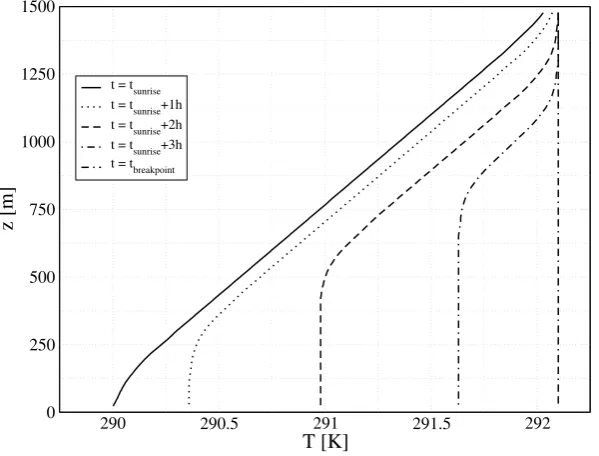
During the morning, the stable core is gradually destroyed starting from the bottom (individuated by the height of the CBL, convective boundary layer) until it disappears at the so called “break-point” time (see figure2.1). This condition of well mixed atmosphere corresponds to a constant vertical profile of potential temperature (see also figure 2.2), which is defined as
θ=T
p0
p
R/cp
, (2.1)
where T is the temperature, p the pressure and p0 the reference pressure at sea level;
the ratio betweenR (gas constant) andcP (specific heat at constant pressure) has a value of0.287for dry air.
Figure 2.1.: Removal of the nocturnal stable layer (Whiteman, 1982). a) At sunrise the thermal inversion over the depth of the valley determines a situation of stable atmosphere; b) with the heating of the valley floor the growth of the CBL starts; c) the stable core sinks and upslope flows arise (secondary circulation); d) the well-mixed situation is reached around noon time.
ground, leaving a residual layer above which gradually disappears through the transfer of energy to the layers below.
Figure 2.2.: Qualitative evolution of a) potential temperature and b) CBL and IT.
terrain; however, a global approach is suitable for models working on large scales or in case fine-grained input are not available.
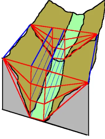
Required inputs for a streamtube model are the valley geometric characteristics, the release rate as a function of time and space, the along-valley wind speed as a function of time, and the sensible heat flux or, alternatively, as in VALDRIFT, the eddy diffusivity. A streamtube model defines the tubes with a geometrical criterion (see figure 2.12): the ratio between the surface of a cell (in the crosswind direction) and the whole valley section
Ωtot is constant at each cross-section of the valley:
Ωjk
Ωtot
=constant, (2.2)
where subscriptsj andkare denote the cross-valley and vertical direction, respectively. Also notice that streamtubes don’t exchange flow in the crosswind direction but only mass due to turbulent diffusion.
The outputs of the model are the pollutant concentrations and the deposition fields as a function of time and space. The dynamical part of the model will not be further discussed here, while the thermodynamic scheme used in VALDRIFT will be extended to the case of a valley of any geometric form; this will allow us to use a global approach (i.e. integrated over the section) not only for the development of the CBL height, but also for the determination of the eddy diffusivity vertical profile. It is worth noticing that the present formulation for the computation of the vertical profile ofKz, which is proposed in
Figure 2.3.: Streamtubes scheme.
2.1.1. Day time
As a first step the evolution of the daily cycle of CBL and IT, averaged over a section of a valley, is simulated, as explained in section2.1. According to Allwine et al. (1996), the variation of sensible heat flux can be written in the form:
dQH
dt =E(t)A0b(z), (2.3)
whereE[W/m2]is the solar radiation entering the atmosphere,A0the fraction ofEwhich
increases the air temperature in the valley, thus modifying the stratification, andb(z) the width of the valley (at height z) which is crossed by the flux F. The structure of E(t) is typically represented through a sinusoidal function:
E(t) =E0sin
hπ
τ(t−ti)
i
, (2.4)
whereτ[s]is the period spanning about half a day (from sunrise to sunset).
The sensible heat per unit length of the valleyQH[J/m]is the sum of two parts, namely
QIT, which is responsible for the decrease of the IT, and QCBL, which causes the CBL
depth to increase. An estimate ofA0 can be obtained through a quite simple heat balance
model ofWhiteman and McKee (1982).
2.1.1.1. Geometric considerations
Let’s consider a section of any form, limited at its top by an horizontal line at height ς
from the valley floor.
The vertical coordinate of the barycenter is defined as:
ηG(ς) =ς− 1
Ω(ς)
Z ς
0 Z b(z)
0
dy z dz, (2.5)
whereΩ(ς) is the cross sectional area
Ω(ς) =
Z ς
0 Z b(z)
0
dy dz. (2.6)
Furthermore, the functionM(ς) is defined as:
M(ς) = Ω(ς)ηG(ς). (2.7) We then assume that the fractions of QH, which may induce a change of the height of
CBL (HC) and IT (HI), are proportional to the width of the valley at the height at which the two layers are positioned at a given timet:
dQCBL
dt =f(HC), (2.8)
dQIT
dt =f(HI). (2.9)
Recalling the first law of thermodynamicsdQ=ρcpTθdθ, the exchanged heat within the
section per unit length, at the height of CBL, can be given the following form:
QCBL(ς) = c0γθ
Z ς
0 Z b(z)
0
γθ(ς−z)dydz
= c0γθM(ς), (2.10)
where the differential of potential temperaturedθis substituted byγθdz,γθ[K/m]being the vertical gradient of potential temperature when the removal of stable layer starts, i.e. at sunrise. Furthermore we set c0 = ρcθpT: the above ratio is nearly constant in vertical
Rewriting equation 2.8 for the CBL (ς = HC), the variation of HC is related to the
variation ofQCBL in the following form:
dQCBL dt = dQCBL dHC dHC dt
= c0γθ dM
dHC
dHC
dt =c0γθΩ (HC)
dHC
dt . (2.11)
For the IT (ς =HI) a similar equation can be derived: dQIT
dt =
dQIT
dHI
dHI
dt =c0γθ
dM
dHI
dHI
dt =c0γθΩ (HI)
dHI
dt . (2.12)
We then assume that the fraction of QS feeding the variation of CBL and IT is
propor-tional to ratio of the width of the section at heightHI and HC, respectively:
dQCBL
dt =
dQH
dt fc
b(HC)
b(HI), (2.13)
dQIT
dt =
dQH dt
1−fcb(HC)
b(HI)
, (2.14)
wherefc is an empirical constant falling in the range 0÷1, which has been introduced
byAllwine et al.(1996) for the partition of the energy flux, in order to decouple equations
2.11and 2.12.
The initial conditions are written as:
(
HC|t=0 =HC0 >0
HI|t=0=HI0 > HC0
, (2.15)
where HI0 is the height over the valley floor of nocturnal stable layer before sunrise
(equation 2.11). When no additional information is available, its upper limit is conven-tionally set at the height of the mountains ridges (provided their elevation is not too high, otherwiseHI0 is set to a lower value). In any case, synoptic flow field over the mountain
ridges is supposed not to interfere with the valley circulation, nor with the heat balance. Equations 2.13and 2.14include different scenarios in the evolution ofHI(t) andHC(t)
according to the values attained by three parameters: the partitioning constant fc, the
width of the valley floor L, and the average inclination of the sidewalls; results are illus-trated in figures2.4,2.5and 2.6.
0.0 0.5 1.0 1.5 2.0 2.5 3.0 3.5 t-t
sunrise [h] 200
400 600 800 1000
z [m]
valle stretta valle larga
pianura
Crescita del CBL e decrescita dell’IT f
c = 0.75
IT
CBL
Figure 2.4.: CBL growth and IT decrease with different valley floor widths andfc= 0.75.
0.0 0.5 1.0 1.5 2.0 2.5 3.0
t-t sunrise [h] 200
400 600 800 1000
z [m]
α = 15°
α = 45°
α = 75°
Crescita del CBL e decrescita dell’IT f
c = 0.75, L = 1000m
IT
CBL
Figure 2.5.: CBL growth and IT decrease with different side slope inclination, fc = 0.75
0.0 0.5 1.0 1.5 2.0 2.5 t-t
sunrise [h]
200 400 600 800 1000
z [m]
f
c = 0
f
c = 1/3
f
c = 2/3
f
c = 1
Crescita del CBL e decrescita dell’IT α = 30°, L = 1000m
IT
CBL
Figure 2.6.: CBL growth and IT decrease with different energy partitioning coefficient, valley floor width L= 1000m and side slope inclination α= 30◦.
with nearly vertical slopes) show a ratio b(HC)
b(HI) →1; as a consequence the heat flux mainly
feeds the CBL; on the contrary in “open” valleys (i.e. with low slope inclination) the core subsidence is more evident, because upslope flow are in this case enhanced. In a very large valley, or in the limit case of flat uniform terrain (L → ∞), energy almost feeds the CBL development, leaving the IT nearly at the initial height. Moreover, the increase of L and tends to delay the “break-point” time, at which the stable core is completely removed. Finally, as one can readily deduce from equations, the lower is HI, the quicker
the “break-point” time is reached.
Some tests were performed on the Adige Valley, in the neighbourhood of Trento (further details on the location are given in section 1.2.1). From a rough analysis of the vertical temperature profile, reported inRampanelli(2004), for this study area a value offc = 0.75
is obtained and adopted in the present work.
As the other parameters is concerned, we can observe that an increase of solar radiation obviously reduces the time required to reach the “break-point”, while an increase of the thermal gradientγθ has an opposite effect.
dH
dt =
A0E(t)
c0γθ
fc
b(HC)
Ω (HC)
. (2.16)
Similarly, substituting equations 2.3 and 2.12 into (2.14), the equation governing the evaluation of the CBL takes the following form:
dh
dt =
A0E(t)
c0γθ
b(HI)−fc
b(HC)
Ω (HI)
. (2.17)
2.1.1.2. Heat balance
An estimate of the fractionA0 of the solar radiation which increases the air temperature
can be obtained through to a thermal balance. The net energy fluxQ∗in the air layer close
to the ground, due to solar incident radiation, can be divided in two contributions: the first,K∗, is due to short wave radiation, and the second,L∗, is due to long wave radiation.
In turn, these contributes can be separated into ingoing and outgoing fluxes, as follows:
K∗ =K ↑+K ↓, (2.18)
L∗=L↑+L↓, (2.19)
whereK↓ is representative of nearly the totality of solar incident radiation and can be again divided in direct and diffused radiation. A part of the incident radiation is reflected and is indicated by K ↑, so that K ↑=−aK ↓, where ais the albedo of the ground and
K∗ = (1−a)K ↓. In the same way, long waves, where the infrared bandLIcovers the large
part of energy (L∗'LI), are identified by the radiation fluxL↑outgoing from the earth’s
surface. In fact L ↓ can be neglected since it is typically much lower than the incident short wave flux, such thatLI'L↑.
During night-time the solar irradiation vanishes, whileL∗ is important and, depending
on the ground cooling, it may tend to sign reverse. The term L ↓ represents the heat release from the ground to the close atmosphere, through irradiation.
Q∗ = K∗+L∗
= (K ↑+K ↓) + (L↑+L↓)
' (−aK↓+K ↓) +L↑
' (1−a)K ↓+LI, (2.20)
whereL↑has been replaced byLI. In the above equations negative values indicate fluxes outgoing from the earth’s surface, while positive values indicate ingoing fluxes: therefore during the dayQ∗<0, while during the nightQ∗>0.
Notice that the backward radiation by the ground, in the infrared band can be estimated as LI
ρcp = 0.08K·m/s, while it vanishes for covered sky.
The fluxQ∗ supplies other physical phenomena as atmospheric turbulence, evaporation
and, more in general, the cooling or heating processes by convection and conduction of all the bodies adjacent to the ground.
Now, considering the heat balance of all the fluxes at the surface, we can write:
Q∗+QG+QE+QH = 0, (2.21)
whereQG is the storage heat flux in the ground, QE is the latent heat flux referred to
evaporation (QE <0) and condensation (QE >0),QH is the sensible heat flux responsible for temperature variation of the atmosphere and convective processes. If the air is perfectly dry, the termQE is null and the termQG can be computed using an empirical expression,
likeQG'0.3QH (Tampieri,1997), which implies:
QH ' −10
13Q∗. (2.22)
In the thermodynamic model developed byWhiteman and McKee(1982)A0 is the
frac-tion of solar radiafrac-tion converted in sensible heat that contributes to the CBL development, under the hypothesis of nearly dry air,A0 can be estimated as
QH
Q∗
, which attains a value
of0.77, according to the above assumptions. It is worth noticing that this value is larger with respect to that one measured byWhiteman and McKee (1982) during surveys in the Brush Creek Valley (Colorado), i.e. A0 '0.3; this is probably due to the difference both in
290 290.5 291 291.5 292 T [K]
0 250 500 750 1000 1250 1500
z [m]
t = t sunrise t = t
sunrise+1h t = t
sunrise+2h t = t
sunrise+3h t = t
breakpoint
Figure 2.7.: Time evolution of potential temperature vertical profile.
2.1.1.3. Temperature and eddy diffusivity profile
Having computed the time evolution of HC and HI through numerical integration, we
can now determine the atmospheric stability and, consequently, the turbulent diffusivity vertical profile (averaged over the width of the valley), which depend upon these two heights. In fact, following the approach adapted fromRampanelli(2004), it is possible to estimate the time evolution of potential temperature through the following expression:
θ(t, z) = θmax−γθ[HI(t)−z] +γθ[HC(t)−z]
−γθ
I ln{2 cosh [I·HI(t)−I·z]}+
γθ
I ln{2 cosh [I·HC(t)−I·z]},(2.23)
where the initial condition is defined asθmax= θ|z=H
I0,t=0andIrepresents the intensity
of variation (i.e. the local vertical gradient ofθ) at the heightHCandHI. Converting then
theθ-profile (figure2.7) to theT-profile using equation 2.1(figure2.8), one can apply the so called “heat budget method” which allows to compute eddy diffusivity profile (figure
278 280 282 284 286 288 290 292 T [K]
0 250 500 750 1000 1250 1500
z [m]
t = t
sunrise
t = t
sunrise+1h
t = t
sunrise+2h
t = t
sunrise+3h
t = t
breakpoint
Figure 2.8.: Time evolution of temperature vertical profile.
Kz(t, z) =
Rz
0 cpρ(ζ)b(ζ)
∂T(t,z)
∂t dζ
cpρ(z)b(z)∂T∂z(t,z)
. (2.24)
Implicit in this procedure is the assumption that the flux of energy crossing an horizontal plane equals the energy storage below it.
2.1.2. Night-time
0 2 4 6 8 10 12 14 16 18 20 22 24
K z [m
2 /s]
0 250 500 750 1000 1250 1500
z [m]
t = t
sunrise
t = t
sunrise+1h
t = t
sunrise+2h
t = t
sunrise+3h
t = t
breakpoint
Figure 2.9.: Time evolution of eddy diffusivity vertical profile.
2.2. The local approach
An alternative method for the calculation of atmospheric turbulent diffusivity over com-plex terrain during day-time is presented herein, which may improve the predictions based on diagnostic meteorological models. The proposed procedure takes into account the geo-graphic location of the area (latitude and longitude), the time of the day, the inclination and exposition of the surface, the soil type and the cloud cover. These data are used to compute the amount of solar heat flux contributing to the heating of the air mass above the ground level, and, consequently, the atmospheric turbulence. The model accounts for the effect of shadows generated by mountain profiles, which determine a differential heating at the valley floor and induce spatial and temporal variations of turbulent diffusivity. Model calibration has been performed through ground data collected during a field campaign in the Adige valley in the surrounding of the town of Trento.
2.2.1. Introduction
often neglected. However, shadows generated by mountain profiles may strongly affect the heating of the air mass along the valley floor, which may differ substantially from the case of flat uniform terrain. As a consequence, secondary circulations are generated, which cannot be reproduced through diagnostic numerical model unless a suitable method for the calculation of distributed heat flux is included.
The proposed method has the aim to compute the atmospheric diffusivity over complex terrain during day-time, which accounts for the orographic factor. Two novel features are included:
• shadowed areas do not contribute to the heating of the air mass above the ground level;
• spatial variations of energy flux at ground level due to the local inclination with respect to solar beams are taken into account.
The first aspect implies that the model must be able to recognize whether each point of the terrain is shadowed by some other point of the domain, at a given date and time. To include the second effect a correction for the relative angle between the solar beams and the ground is computed at each point of the digital elevation model. As a consequence the distribution of global radiation is no more constant over the domain, but varies, at a given time, depending on the local exposition. Hence, the spatial distributions of net radiation, sensible heat flux and turbulent diffusivity change accordingly.
The surface energy balance is closed using different well known formulations in terms of local values of parameters (Holtslag and van Ulden,1983) and taking into account the spatial variability of the relevant parameters. The model also considers that the absorption coefficient varies with the inclination of solar beams, depending upon the time of day.
Required input data for the model are:
• the digital elevation model of the area with a suitable resolution;
• land use categories or, alternatively, the distributed albedo coefficient and roughness length;
• the global radiation at ground level measured by one or more weather stations (which is required, at least, for calibration) or, alternatively, the cloud coverage.
Figure 2.10.: Study area and location of measurement and test points.
and the vertical turbulent diffusivity at ground level. For the present study a height of3m
m above the ground has been adopted.
The model is tested through the inclusion of the proposed procedure within the code of CALMET, a meteorological diagnostic mass-consistent preprocessor which computes the 3D fields of wind and temperature (Scire et al.,1999). In its original formulation the code considers that mountains can influence the wind field, but not the solar radiation at ground level (and consequently the other quantities). In testing the model, the spatial and temporal variations of turbulent diffusivity are determined both with the standard procedure and including the effect of orographic factor. Calibration has been carried out by comparing the values estimated through the described procedure with those obtained with a sonic anemometer during a field campaign.
The study area is a part of the Adige Valley in the surrounding of the town of Trento (Northern Italy), characterized by an average latitude ϕ = 46◦N and average longitude
λ = 11◦E; the size of computational domain was 10×20km, with a cell resolution for computation of 100m. The location of measurement and test sites used in present study is indicated in figure2.10:
• 2: Trento airport (radiometer + test site),
• 3: Ischia-Podetti, West side of the valley (sonic anemometer + test site),
• 4: valley center (test site),
• 5: East side of the valley (test site).
2.2.2. Formulation of the model
2.2.2.1. The solar path
The definition of shadowed regions and the computation of local aspect and inclination with respect to solar beams preliminarily requires the reconstruction of the solar path. The position of the sun is calculated in terms of a mean value of latitude/longitude of the domain, day of the year, time of the day, local aspect and inclination of the surface. The extraterrestrial radiation is written as
E=S0fsinγ, (2.25)
where a correction factor f is included which takes into account the variation of the sun-earth distance during the year due to orbit ellipticity. In (2.25) γ represents the angle between the solar beam and the local tilted surface and S0 = 1370W/m2 is the solar
constant.
Spencer(1971) relationship is used to compute the factorf, which reads:
f = 1.0011 + 0.034221 cosd0+ 0.00128 sind0
+0.000719 cos 2d0+ 0.0000077 sin 2d0, (2.26)
where
d0 =
360
365(d−1), (2.27)
and drepresents the Julian day.
In case of flat horizontal surfaceγ = 90−ξ, whereξ is the zenith angle, which is given by (Iqbal,1983):
Figure 2.11.: Sketch of the defined angles and notation.
which reads:
ω = 180
12
t−12 +λ−λmrd
15
. (2.29)
In equation 2.29λmrd represents the longitude of the central meridian of the local time
zone andt is time. Furthermoreδ can be expressed as
δ= 23.45 sin
360
365(d−81)
. (2.30)
The correction for tilted surface is computed through the following expression (Allwine and Whiteman,1986):
sinγ = sinδcosϕcosκsinυ−cosδsinωsinκsinυ
+ cosδcosϕcosωcosυ+ sinδsinϕcosυ
−cosδsinϕcosωcosκsinυ, (2.31) whereυrepresents the local value of surface tilt angle (υ= 0◦ →horizontal, υ= 90◦ →
vertical) andκis the local surface aspect (κ= 0◦ →facing North,κ= 90◦→ facing West,
κ= 180◦ → facing South,κ= 270◦→ facing East).
2.2.2.2. Shadow and sky view factor
have a sky view factor smaller than those located on top of the mountains. In the present model the sky view factor is locally defined as follows :
Sv =
R2π
0 cos [φ(λ)]dλ
2π , (2.32)
where φ is the minimum elevation angle, measured from the horizontal plane, beyond which solar beams cannot reach the given location at the ground. It is also assumed that zones which are hidden by mountain profiles during day time are only subject to the diffuse fraction of global radiation entering the atmosphere (see below).
2.2.2.3. Global radiation
The computation of local values of global radiation requires the estimate of the clearness indexKt, which is defined as the ratio between the global radiation at the groundRGand the extraterrestrial radiationE:
Kt= RG
E . (2.33)
In order to compute global radiation the procedure introduced by Erbs et al. (1981) is used. Two indexes can be defined, iR and dR, which represent the fraction of incident direct radiation and of diffuse radiation, respectively. They read:
iR =
RI
RG, (2.34)
dR =
RD
RG. (2.35)
In terms ofiR anddR the global radiation is then written in this form:
RG=RI+RD =RG(iR+dR) =EKt(iR+dR), (2.36)
whereE is the computed extraterrestrial radiation,RI is the incident direct radiation and RD the diffuse radiation.
Equation2.36 is valid in case of flat uniform terrain. Under this condition the value of
RG at a given site, according to Erbs et al.(1981) formulation:
iR = 1−
p
cosξ, (2.37)
dR = p
cosξ, (2.38)
whereξis the zenith angle. The coefficientpdepends on the clearness indexKtaccording
to the following expressions:
p= 1−0.09Kt Kt≤0.22
p= 0.9511−0.1604Kt+ 4.388Kt2−16.638Kt3+ 12.336Kt4 0.22< Kt<0.80
p= 0.165 Kt≥0.80
.
(2.39) For complex topography it is assumed that the diffuse radiation is proportional to the local values of the sky view factorSv; hence, a modified version of (2.36) is adopted, which
takes the following form:
R0G=RI+RD0 =RG(iR+SvdR) =EKt(iR+SvdR). (2.40) In this caseKtis estimated in terms of the measured value of global radiationR0Gat a site through (2.40), where we setSv =Sv,m,Sv,mbeing the sky view factor of the measurement
point, and we use equations2.37,2.38 and 2.39 to computeiR anddR. Furthermore, the
values ofiRanddRare assumed to be constant over the whole domain at a given time (i.e. at a given solar zenith angle). Hence, once the value ofKt has been determined, equation
2.40can be used to compute the global radiation R0G at a given site in terms of the local value of the sky view factor.
When the measure of Kt is not available (or not reliable), empirical formulations can
be used to compute the global atmospheric trasmissivity; however, they do not account for the sky view factor, nor for the splitting between diffuse and incident radiation. An example is the following formula
fraction. Notice that in this case the global radiation at a site is simply calculated as:
R0G=RG=EKt. (2.42)
2.2.2.4. Sensible heat flux
The sensible heat flux represents the part of energy budget which effectively contributes to the heating of the air mass above valley floor. Its computation preliminarily requires the estimate of the net radiation Q∗. In the present model a modified expression with
respect to the original formulation ofHoltslag and van Ulden (1983) is used, which takes the following form:
Q∗ =
(1−a0)R0G+c1T6−σT4
1 +cH . (2.43)
Notice that equation 2.43 doesn’t include the additional term proportional to cloud coverage. In fact, according to the present procedure, the filtering effect and the diffuse radiation effect of cloud cover are already included in the computation ofR0G.
In (2.43) the correction for the albedo with respect to solar elevation is accounted for, using the expression ofPaltridge and Platt (1976):
a0 =a+ (1−a) exp−0.15(90−ξ)−0.5(1−a)2; (2.44) furthermore σ is the Stefan-Boltzmann constant, c1 = 5.31·10−13W/ m2K6
is an empirical constant andcH ranges about0.12; according to van Ulden and Holtslag(1985)
andHanna and Chang(1992),cH is found to depend on soil type and moisture.
The sensible heat fluxQH is then computed using the following formula:
QH = rB
1 +rB(1−cg)Q∗, (2.45)
whererB is the Bowen ratio, which mainly depends on soil moisture, andcg is a function of the properties of the surface, for which Oke (1982) suggests a value ranging between
0.05 and 0.25 for rural areas, or between 0.25 and 0.30 for urban areas. In the present work a constant value of cg = 0.20 is used for the whole domain, while the default values of the Bowen ratio suggested in the original code of CALMET are kept.
2.2.2.5. Turbulent diffusivity
In the present model the Monin Obukhov lengthLand the friction velocityu∗are computed
iteratively from the output values of temperature, T, and wind field, u, generated by CALMET, using the following expressions (Panofsky and Dutton,1984):
LM O = −
ρcpu3∗T
kgQH
, (2.46)
u∗ =
ku
lnzz
0 −Ψ
z L
+ Ψ z0 L
. (2.47)
wherekis von Karman constant, ρ is the air density,cp is the specific heat at constant pressure,g is gravity, z is the reference height (z= 3m over the local surface is adopted in the present work), andz0 is the roughness length. The similarity functionΨ is the one
defined in equation 1.7. Finally, the similarity law for vertical turbulent diffusivity given in equation1.19is adopted:
Kz(z) = ku∗z
Φ . (2.48)
0 200 400 600 800
R
g
[W/m²]
site 1 - radiometer site 1 - model
0 2 4 6 8 10 12 14 16 18 20 22 24
t [h] 0
200 400 600 800
R
g
[W/m²]
site 2 - radiometer site 2 - model
0 200 400 600 800
R
g
[W/m²]
site 1 - radiometer site 1 - model
0 2 4 6 8 10 12 14 16 18 20 22 24
t [h] 0
200 400 600 800
R
g
[W/m²]
site 2 - radiometer site 2 - model
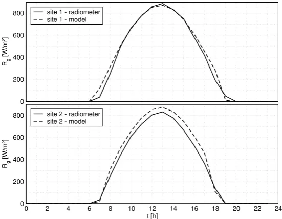
Figure 2.13.: Global solar radiation in a sunny day: comparison between computed values and data registered by radiometers 1 and 2 (see figure 2.10).
2.2.3. Results
The values of model parameters (cg = 0.20,cH = 0.12) have been determined through the
calibration of computed global solar radiation based on the whole set of data (one year) from two radiometers in the study area (denoted as site 1 and 2 in figure2.10). Computed values ofRG, based on the above estimates, are compared with values of global radiation
registered in a cloudy day and in a sunny day in figures 2.12 and 2.13, respectively. The computed global radiation in a sunny day evaluated at different locations across the Adige Valley is shown in figure2.14: the time shift exhibited by the daily distributions at different locations clearly reflects the effect of shadows generated by mountain profiles.