Effects of the Income Stabilization Tool on farm income level, variability and concentration in Italian agriculture

R E S E A R C H

Open Access

Effects of the Income Stabilization Tool on

farm income level, variability and

concentration in Italian agriculture

Simone Severini

, Giuliano Di Tommaso

and Robert Finger

* Correspondence:severini@unitus.it

1

Tuscia University, Viterbo, Italy Full list of author information is available at the end of the article

Abstract

This paper provides an ex ante assessment of the effects of the Income Stabilization Tool (IST), a new risk management tool proposed in the Common Agricultural Policy of the European Union. We investigate the effects of IST on income variability and levels as well as on income inequality in the farming population. We take Italian agriculture as an example as the introduction of IST is currently under discussion there. A rich panel of 2777 farms was studied over a period of 7 years. We use stochastic simulation to derive different income inequality estimates and apply Gini decomposition approaches to assess the distributional implications of IST. We compare the current income situation with that resulting from a hypothetical implementation of IST under different policy scenarios, also accounting for reduced levels of CAP direct payments. We find that IST not only stabilizes farm income but also enhances its level and reduces income inequality in Italian agriculture. IST is more effective in reducing income inequality when farmers pay contributions to mutual funds that are proportional to their income compared to the case of flat rate contributions. Finally, results do not support the hypothesis that the impact of IST will differ if the level of direct payments were to be reduced. Thus, results seem robust enough to accommodate future policy conditions.

Keywords:Agricultural policy, Income inequality, Income Stabilization Tool, Direct payments, Risk management

JEL classifications:D63, G22, Q12, Q18

Introduction

Current and future developments foreseen by the Common Agricultural Policy of the European Union (CAP) point in several directions, comprising (1) a shift towards more targeted and tailored payments, with particular emphasis on improving provision of a

wide range of ecosystem services; (2) a reduction of support based on direct payments1;

and (3) increasing support of market-based instruments to cope with the high and

growing risk exposure of farms (e.g., Bureau et al., 2013, Galán-Martín et al., 2015,

Meuwissen et al., 2018, Fresco and Poppe, 2016). Regarding the latter, the EU Rural

Development Policy provides financial contributions (Bardaji and Garrido, 2016): to

© The Author(s). 2019Open AccessThis article is distributed under the terms of the Creative Commons Attribution 4.0 International License (http://creativecommons.org/licenses/by/4.0/), which permits unrestricted use, distribution, and reproduction in any medium, provided you give appropriate credit to the original author(s) and the source, provide a link to the Creative Commons license, and indicate if changes were made.

1

premiums for insurance against economic losses to farmers, to mutual funds to pay financial compensations to farmers for economic losses, and to mutual funds managing an Income Stabilization Tool (IST) providing compensation to farmers

for a severe drop in their income2. The focus of the paper is on the IST in Italy.

Currently, Italy as well as Hungary and the Spanish region of Castilla y Leon are evaluating the possible implementation of this innovative tool. Yet it is not estab-lished in any of these countries, requiring ex ante assessments of possible

implica-tions (Bardaji and Garrido, 2016).

Existing studies on IST focus on its income-stabilizing effect (i.e. risk reduction), governmental costs, and potential beneficiaries within the farming population (EC,

2009; dell’Aquila and Cimino, 2012; Liesivaara, Myyrä and Jaakkola, 2012; Liesivaara

and Myyrä, 2016b; Pigeon, Henry de Frahan and Denuit, 2012; Mary, Santini and

Boulanger, 2013; Severini et al.,2018; Trestini et al.,2017 and2018). Moreover, effects

on farm income concentration have been provided (e.g. Finger and El Benni 2014a).

Yet these studies have not addressed potential interdependencies between IST and direct payments and changes therein. Direct payments also influence income levels, stabilize farm income, and reduce income disparity within the farm population

(Enjolras et al., 2014; Severini et al.,2018; Severini et al.,2016a and 2016b; El Benni

et al.,2012; El Benni et al.,2016)3. Thus, the impact of IST could differ under different levels of direct payments.

In this paper, we contribute to the literature by providing an ex ante assessment of this tool for Italian agriculture. The aim of the analysis is to jointly quantify the potential effects of IST on income variability, income level and income concentration to provide a multidimensional assessment of this tool. Furthermore, this is done not only under the current situation but also under different direct payment reduction scenarios.

We use a panel data set for Italian agriculture consisting of 2777 farms observed over a period of 7 years. This allows an assessment of the distributional implications of IST by combining stochastic simulation, the estimation of various income distribution indi-cators and a Gini decomposition approach. The analysis compares the current income situation with that potentially resulting from the implementation of IST.

The remainder of the paper is organized as follows. The next section provides an

explanation of the functioning of the IST.Methodology and datadescribes the

method-ology and the data used. Results and discussion presents and discusses the results of

the analysis, while conclusions are put forward in the last section of the paper.

Background on the functioning of the IST and its impact on farm income The IST is of particular interest to policy-makers because (1) it focuses on the key vari-able of interest, i.e., income; (2) it implicitly accounts for various correlations between prices and yields and across profits of different farm activities; (3) subsidization of IST complies with WTO green-box requirements; (4) it can also cover systemic risks (specifically price risk) that are not covered by purely commercial insurances thus

2

Art. 39 of Regulation (EU) No. 1305/2013 of the European Parliament and of the Council of 17 December 2013 on support for rural development by the European Agricultural Fund for Rural Development (EAFRD) (OJ L 347, 20.12.2013).

3_{Reducing income disparity between EU Member States is another objective that is not considered in this}

hampering the principles of risk pooling, (5) it is based on a public-private partnership

(e.g., Bardají and Garrido, 2016; El Benni et al., 2016, Mary et al., 2013, Meuwissen

et al.,2003,2008,2011,2013; Liesivaara and Myyrä2016a).

The IST schemes are going to be managed by mutual funds accredited by member states for farmers to insure themselves. A mutual fund creates a financial reserve through annual farmer contributions (regulated by each fund) and, if adverse events lead to income losses exceeding the threshold, the mutual fund compensates losses experienced by farmers. The rationale for the mutual fund is to deal with risks that are

beyond the individual farmer’s capacity to cope with (Cordier and Santeramo, 2018).

Larger and more diverse mutual funds reduce the probability of occurrence of a large amount of indemnities to be paid in a specific year and thus also the costs for re-insurance (Severini et al., 2019). However, mutual funds restricted to farmers belonging on a specific sector and/or region may have the advantage reduce moral hazard prob-lems because a less asymmetric distribution of information (Trestini and Giampietri, 2018).

The indemnification is defined as follows:

Ind¼ _β0 _ðE−IÞ if_if I_I≥_<IR_I

R

ð1Þ

whereIis the realized income for the year under consideration andE(I) is the average

income realized in the previous 3 years (see Finger and El Benni2014bfor discussions)

and is calculated as follows:

E Ið Þ ¼1

3

X_t−1

t−3It ð2Þ

IRis the reference income that triggers indemnification for the year under

consider-ation and it is defined asIR=α∙E(I), whereαis lower than one (e.g., 0.7) and reflects a deductible.

The coverage rate of IST is βso that the indemnification paid is only a share of the

actual income gap. These deductibles are used at two stages, i.e., the loss required to

trigger a payout and a farmer’s participation in the losses covered. Both deductibles

reduce moral hazard behavior. The IST is going to have an impact on level and stability

of farm income. Income of a generic farm for a given year is stochastic in nature (~_I)

and can be represented as:

~_I¼MIfþDPþIndf−Cont ð3Þ

where MI is market income generated by the production activities net of CAP directf

payments (stochastic because of production and price uncertainty) and DP is overall amount of CAP direct payments (deterministic, i.e., known to farmers).

When IST is in place, a farmer’s income also includes the last two terms of (3): the

indemnification and farmer contribution to the mutual fund (i.e., similar to an insur-ance premium). The sum of these two terms can be defined as the net financial benefits

accruing to the respective farm derived from IST (i.e., NBIST = Ind−Cont). This can

This brief discussion of the potential income consequences of IST reveals some policy-relevant aspects. Firstly, IST is expected to reduce income variability. The prob-ability of receiving indemnification and its level depends on several factors, including the distribution of farm gross margin as well as the extent of direct payments. Direct

payments stabilize farm income (e.g., Cafiero et al., 2007; Finger and Lehman, 2012)

since they are mainly derived from fully decoupled payments that are a relatively stable

source of farm income (Severini et al.,2016b). Therefore, a large amount of direct

pay-ments is expected to lessen the likelihood that farm income will fall below the reference income level and will receive indemnities. This suggests that it would be interesting to assess the impact of the implementation of IST under different levels of direct payments.

Secondly, while the net financial benefit derived from IST is negative for farmers who do not receive indemnifications, the financial benefit for the overall group of farms is positive given that a share of the indemnifications is covered by public funds. This means that IST provides support to the overall group of farmers by enhancing their

average income4.

Thirdly, as some farmers benefit from the IST because recipients of indemnifications, the others are negatively affected, the support provided by IST is not equally distributed among the farming population. Hence, IST is expected to have income distributional consequences. More specifically, if farms with lower expected incomes (e.g., Finger and

El Benni, 2015, El Benni et al., 2016) are more likely to receive indemnification, the

income inequality in the farming population can be presumed to decline.

Finally, the way farmers’ contribution to the mutual fund is defined also affects how

farm income is distributed within the farm population. The costs of the indemnifica-tions not covered by public funds can be distributed among farmers according to differ-ent rules such as a uniform flat per farm contribution or a contribution proportional to the average income level of each farm. The two approaches are expected to result in a different distribution of costs and benefits of the IST.

Methodology and data

Motivation of the methodological approach

We empirically test and quantify the potential short-term consequences of the application of IST by using a large sample of farms. This allows us to provide nationwide results and to address income inequality consequences of IST that clearly requires a large sample of

farms if useful insights are to be obtained (e.g., Finger and El Benni, 2014a; Liesivaara

et al.,2012; Mary et al., 2013; Severini et al.,2018). We focus on a simulation approach

that is applicable to a large sample (e.g., Keeney,2000; El Benni et al.,2016; Severini et al.,

2018) instead of focusing on a farm-modeling approach which usually concentrates on a

few representative farms (see e.g., Turvey, 2012; Castañeda-Vera and Garrido,2017). As

in previous analyses (e.g., Severini et al.,2018; Finger and El Benni,2014aand b; El Benni,

Finger and Meuwissen, 2016; European Commission, 2009; Liesivaara, Myyrä and

Jaakkola, 2012), we assume mandatory participation, as the question of participation is left

open by the EC. Along these lines, Matthews (2010) remarks that, given the substantial

4_{Participation in IST could also generate transaction costs that negatively affect farm income. Therefore,}

public subsidy involved in CAP risk management tools (such as IST), not many farmers would opt out of such a scheme.

The effect of IST on production choices is not modeled5. Hennessy (1998) provides a

theoretical framework to analyze the impact of income support policies under uncer-tainty. A farmer is assumed to maximize his/her expected utility of income (profit) which also includes government support such as the CAP direct payments (which are mostly decoupled from production). However, IST will also provide support to farmers.

As shown by Hennessy (1998), even if the amount of support were fully decoupled

from production choices (e.g., input use), it still influences producers’ choices if the

expected marginal utility depends on the level of profits. Indeed, if the support was dependent on the source of uncertainty, as it is clearly in the case of IST, this may

cause an increase in production (input use) (Moro and Sckokai, 2013). Despite the

potential relevance of this issue, very few analyses have assessed the potential

implica-tion of IST on farmers’production choices (e.g., Mary et al.,2013) or decisions

regard-ing the use of alternative risk management tools (Lougrey et al., 2016; Castañeda-Vera

and Garrido,2017). All these studies listed above refer to a very limited number of

indi-vidual or representative farms neither allowing to extend results to the whole farm population nor analyzing income distribution consequences (e.g., Finger and El Benni, 2014a; Liesivaara et al.,2012; Mary et al., 2013; Severini et al.,2018). There is a

trade-off between the detailed representation of farmers’ decision and the number of farms

considered, especially due to data limitations and requirements to consider farm-specific

decision-making under risk (e.g., Turvey,2012; Mary, Santini and Boulanger,2013).

Empirical strategy to assess income consequences of IST

The effect of IST is assessed by comparing the observed income (i.e., including CAP direct payments but without IST) with the income that could be generated with IST in place in each of the farms in the sample. We consider three different scenarios

described in Table1.

The baseline scenario I, i.e., with direct payments but without IST, reflects current

conditions as observed in our sample. We assume a single nationwide mutual fund will

manage the IST (see Severini et al. (2018) for discussions and alternative specifications

of the mutual fund). Farmers have to pay a contribution to the mutual fund. In scenario

IIF and IIP (Table 1), farmers pay contributions that are set to recover 35% of the

indemnifications paid by the mutual fund provided that up to 65% of these is covered

by public funds6. Farm-level contributions to IST are not yet legally specified. Thus,

two scenarios are used. Firstly, as proposed by Finger and El Benni (2014a), we simply

5

Future research could explore the potential impact of IST on the behavior of risk-averse farmers. However, this requires a relatively large amount of additional data including, primarily, the extent of the farmers’risk aversion and this data is currently not available. Note that farmers are expected to have different risk prefer-ences (see e.g., Iyer et al.,2019, for an overview). Therefore, it would be inappropriate to apply the same risk aversion level to all farms as simulation results would be strongly driven by the imposed assumptions.

6_{The main simulation assumes that there are no additional costs to be charged to farmers. However,}

divide the 35% of the total indemnifications paid by the mutual fund in each of the

years (TIndt) by the number of farms in the sample (n):

ContF_t ¼0:35TInd_t=n ð4Þ

ContFtis the flat rate contribution paid by the farmers to the mutual fund (IIF in

Table 1). In a specific year, each farm pays the same contribution regardless of its size

and the probability that it will receive an indemnification. Flat rate insurance premiums are used, for example, in the catastrophic crop insurance program in the USA (e.g., Shields,2015).

However, when farms vary markedly in terms of size, as in the case of Italy, it seems

very unlikely that all of them will be charged the same amount7. Therefore, in scenario

IIP we calculated farm-specific contributions by distributing the IST cost charged to farmers in proportion to their average income. The proportional contribution paid by thei-th farmer in thet-th year is calculated as:

ContPit¼0:35 ðTIndt=TEtÞ Eit ð5Þ

where TEtis the sum of the average incomes of farmers.

Hence, TIndt/TEtreflects the average indemnification rate of IST in yeart. Note that

such configuration seems more appropriate for the case of Italy. Therefore, the discus-sion of the results will focus only on this scenario.

Finally, an additional scenario considers the hypothetical case in which IST is fully

subsidized (IIin Table1). While this scenario is ruled out by EU Regulation, it is used

to isolate the impact of the role of the farmers’ contributions by comparing results

referring to scenarioIIwith that of scenariosIIFandIIP.

The consequences of the implementation of IST have been assessed also under scenarios considering reduced levels of direct payments. These scenarios have been developed by applying the same relative reduction (%) to the level of direct payments

received by each farm in the baseline conditions8. This simulation exercise allows to

assess the impact of IST in hypothetical conditions of lower direct payments support. This is justified by the fact that, according to the recently proposed Multiannual

Finan-cial Framework for the period 2021–2027 (European Commission, 2018), the level of

direct payments will likely be lower than in the past.

Table 1Description of the simulation scenarios referring to the implementation of the IST

Code Description

I Baseline: current observed situation, including CAP direct payments, but without the IST in place IIP IST with farmers paying a contribution proportional to their income to the mutual fund IIF IST with farmers paying a flat rate contribution to the mutual fund

II Theoretical case in which the IST is fully subsidized (i.e., farmers do not pay any contribution to the mutual fund).

7

This also seems to comply with actual practices in subsidized farm insurances whereby the premium is defined as a share of the value of the insured production (Bardají and Garrido,2016; Castañeda-Vera and Garrido,2017).

8_{Reducing direct payment not uniformly within the farm population (e.g., more in some types of farming}

Approaches used in the analysis

The income stabilization effect of IST is assessed using the coefficient of variation of farm income calculated for each individual farm over the years from 2012 to 2015. The income enhancement role of IST is assessed by simply comparing the average income level of the farms in the sample over the same period. In both cases, the analysis is based on the comparison of the conditions with and without IST in place.

Income distributional consequences of IST are assessed using three approaches. First, to allow for robust policy conclusions, three different measures of income inequality

are used (see also Finger and El Benni 2014a): (1) the Gini coefficient, (2) the Theil

index, and (3) the 80/20 quintile share ratio (the ratio of the top and bottom 20%

income percentile)9. To conduct pairwise comparisons among the IST specifications

considered, non-parametric bootstrap (N = 1000) was used to derive confidence

inter-vals for the inequality measures (Efron, 1993). These serve to test for significant

differ-ences among the inequality measures calculated for the different IST specifications by means of one-way ANOVA with the Scheffé-adjusted significance levels (Scheffé,

1959). Because results from these different income inequality measures yield similar

results, in the text we only refer to the Gini coefficient. Results regarding the other

measures are reported in the Appendix (Table 7).

Second, the consequences of IST are observed on two groups of farms: those that would have received and those that would not have received IST indemnifications based on their income development observed in the past.

The third approach used to assess the income distributional consequences of IST is the Gini decomposition by income source (Pyatt et al., 1980; Lerman and Yitzhaki,

1985; Keeney, 2000; Ciliberti and Frascarelli, 2018). When income is generated by k

components, the Gini coefficient can be decomposed as follows10:

G¼XK_k¼1RKGKSK ð6Þ

Rkdenotes the“Gini correlation”between income componentkand the rank of total

income. This is given by the covariance between income from the k-th income

compo-nent and the rank of total income, divided by the covariance between income from this

component and the rank of this same income component (Pyatt et al.,1980): cov(yk,F)/

cov(yk,Fk). Moreover,Gk denotes the Gini coefficient for thek-th income component.

Finally,Skdenotes the income share of thek-th income source.

The product between Rk and Gk gives the concentration coefficient of the k-th

income source (Ck). It measures how income from each source is transferred across a

9

The Gini coefficient measures twice the surface between the Lorenz curve (this maps the cumulative income share against the distribution of the population ranked from poorest to richest) and the line of equal distribution. It ranges from 0 (perfect equality) to 1 (perfect inequality). The Theil is a class of general entropy measure. We use the following formulation:T¼1

N

PN i¼1

yi

y1 nðyi

yÞwhereNis the number of the individuals considered,yiis the income level of thei-th individual andyis the average income of such

individuals. The values of this index vary between 0 and∞, with zero representing an equal distribution and a higher value representing a higher level of inequality. The 80/20 quintile share ratio is the ratio of the top and bottom 20% income percentile. It reveals how much richer the top 80% of the population is in comparison with the bottom 20% of the population. It ranges from 1 and∞, with 1 representing an equal distribution and higher values representing a higher level of inequality. See Finger and El Benni (2014a) for further details.

10_{With a substantial incidence of negative incomes,G(I) may become overstated, perhaps reaching values}

population that is ranked according to the level of total income received by each of its members.

Equation (6) shows that each income component influences income concentration

depending on the importance of that source of income (Sk), how it is distributed among

the sample (Gk), as well as the level of the“Gini correlation”between this income

com-ponent and the rank of total income (Rk) (Stark et al.,1986).

Pyatt et al. (1980) and Lerman and Yitzhaki (1985) developed a measure that

parti-tions the overall inequality into contributing components. In the case of income, this

allows an assessment of the “proportional contribution to inequality” of the k-th

income source:

PK¼ðRKGKSKÞ=G ð7Þ

The marginal impact of a single income component on income inequality can be

derived using the Gini coefficient rate of change with respect to the mean of k-th

income component (Lerman and Yitzhaki,1985):

dG dμk

¼1_μðCk−GÞ ð8Þ

in whichμkis the mean value of the componentk-th of income. This measure permits a

comparison of the marginal contribution of each source of income to the inequality, even if these sources represent different shares of the overall income. In particular, we compare the Gini coefficient rate of change of direct payments with that of the net financial bene-fits generated by IST.

Finally, the Gini coefficient rate of change can be used to derive the elasticity of the Gini coefficient for each income component as follows:

η_k¼μk

G

dG dμ_k ¼

1

G

μk

μðCk−GÞ

ð9Þ

This measures the impact of a 1% change of a single income source on the income concentration, assuming that the internal ratio between the total income distribution

and the mean of the income source is undisturbed (El Benni and Finger,2013, p. 641).

The income of each farm with IST in place is subdivided into the three income sources referred to in (3): market income is calculated by subtracting direct payments from the observed income (MI); amount of direct payments (DP); net financial benefit

of IST (NBIST). This last income component could assume different levels according to

the different configurations of IST previously described. However, the Gini decompos-ition is developed solely based on the hypothesis that farmers pay a contribution proportional to their income (i.e., ContP as in (5))11.

Non-overlapping confidence intervals are used to reject null hypotheses of no differ-ences of marginal impacts across different income sources. Note that the use of 95% confidence intervals results in a much more conservative test than usual tests applied

at the 5% level of significance (see Payton et al.2003for numerical simulations).

11

Data

We use the value added at the farm-level as underlying income variable for the analysis. This is obtained by deducting total intermediate consumption (farm-spe-cific costs and overheads) from farm receipts (total output and public support) and measures the amount available for remuneration of the fixed production factors

(work, land, and capital) (European Commission, 2010). The Italian Ministry of

Agriculture has adopted farm value added as the income indicator to be used for

IST (MIPAAF, 2017). Value added includes direct payments regardless of whether

these are coupled to or decoupled from production.

The analysis is based on a balanced sample of farms which belonged to the Italian

FADN12 consecutively in the years from 2009 to 201513. Data for the period 2009–

2011 is used to identify farms’ average income levels for 2012 according to (3). Thus,

although data from 2009 onwards has been used, 2012 is the first year of simulated application of IST. Fourteen farms with negative average incomes in the considered years were removed from the analysis since negative incomes are usually treated differ-ently in this type of insurance scheme (e.g., in the Canadian AgriStability program,

Kimura and Anton, 2011, see also Finger and El Benni2014a). This yields a balanced

sample of 2777 farms, reflecting around 1/3 of the entire Italian FADN sample. While

it is not possible to state that the sample fully represents the farming population14, the

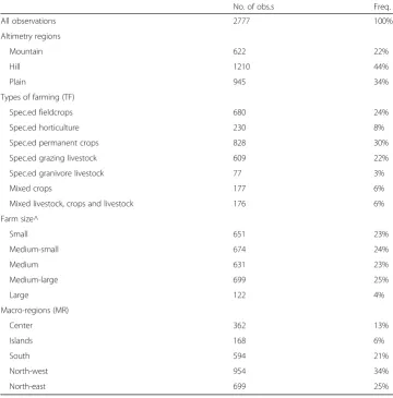
distribution of farms does include important components of this population with respect to geographical location of the farms (i.e., altimetry regions and macro-regions of Italy), farm size, and types of farming (Table2)15.

All monetary figures are deflated to allow comparability among data from different

years by means of the Eurostat Harmonized Index of Consumer Prices (HICP)16.

Results and discussion

Effects of IST on farm income stability, level, and inequality

The main purpose of IST is to stabilize farm income. It reduces the level of variability in farm income over the investigated period by compensating farms which suffer severe

12_{FADN is a very commonly used database in policy analysis within the EU because, according to the}

European Commission (2010), it“is an instrument for evaluating the income of agricultural holdings and the impacts of the Common Agricultural Policy”. It is generally biased towards commercial farms because very small farms are excluded from the survey. However, the sample also contains part-time farms ensuring the representation of several types of farming observed in the population.

13_{CAP reform was introduced in 2015. Hence, from a concept point of view, this year differs from previous}

years in terms of direct payment policy. However, the changes introduced in 2015 were not massive in Italy as the chosen methods of gradual and partial convergence maintain the overall amount of direct payments received by each farm very close to the amount received in the previous period (European Commission, 2015). However, to account for the peculiarity of 2015, results from this year have been compared with those from previous years. Results related to income concentration and the Gini decomposition show that the confidence intervals referring to 2015 overlap with those referring to all previous years. Similarly, results for the whole 2012-15 period do not differ from those referring only to the 2012-14 period (Tables 8 and 9 in the Appendix).

14

The selection of a constant sample may result in a sample bias. However, a constant sample is needed because the analysis of the variability of farm income must be based on data referring to a relatively long period of time

15_{Basic statistics of the farm sample are reported in the Appendix, Table 6.} 16

drops in their incomes. This is underlined if comparing results referring to the current situation (i.e., without the IST) with those resulting from the scenarios in which the IST is introduced (Table1) (Fig.1)17.

IST is highly effective in stabilizing farm income and this is the case even if the level

of direct payments is reduced (Fig.1). As expected, these are also found to play a role

in income stabilization since reductions in direct payment levels result in an increase in relative income variability.

Since IST is subsidized, it enhances the average income level of the farming popula-tion. On average, the income level with IST is higher than without this tool in place.

This is shown in Fig. 2 where the line referring to the average income level with IST

Table 2Number of the sampled farms and their distribution among altimetry regions, types of farming, farm size, and macro-regions of Italy. Balanced sample (year 2015)

No. of obs.s Freq.

All observations 2777 100%

Altimetry regions

Mountain 622 22%

Hill 1210 44%

Plain 945 34%

Types of farming (TF)

Spec.ed fieldcrops 680 24%

Spec.ed horticulture 230 8%

Spec.ed permanent crops 828 30%

Spec.ed grazing livestock 609 22%

Spec.ed granivore livestock 77 3%

Mixed crops 177 6%

Mixed livestock, crops and livestock 176 6%

Farm size^

Small 651 23%

Medium-small 674 24%

Medium 631 23%

Medium-large 699 25%

Large 122 4%

Macro-regions (MR)

Center 362 13%

Islands 168 6%

South 594 21%

North-west 954 34%

North-east 699 25%

^According to economic standard output classes (European Commission,2010)

Source: Own elaborations on Italian FADN data

17

(scenario IIP) is above that referring to the baseline condition (scenarioI) for any level

of direct payments (x-axis)18. Farm income levels decline as direct payments decrease

(i.e., moving right on the x-axis of Fig. 2). These results show that the

income-enhancing role of IST can partially compensate for the income loss caused by possible

cuts in direct payments (Fig. 2). Finally, note that the financial resources distributed by

IST will only increase to a very negligible extent when simulating direct payment

reductions. This is shown by the fact that the two curves in Fig.2 remain more or less

at the same distance regardless the level of cut in direct payments.

The IST causes a re-distribution of resources within the farming population that can lead to a reduction in income inequality. Note that there is a marked differ-ence between how support is distributed by means of IST and direct payments: while the latter are granted to almost all farms, the IST is targeted to support only those farms experiencing large income drops. These differences can be seen graph-ically by considering two groups of farms: farms that are indemnified (ind) and those that are not (no ind). The income gap between these two groups of farms is

very large when IST is not in place (I(ind) < I(no ind)) (Fig. 3). This gap is

re-duced significantly when IST is applied (Fig. 3).

About 20% of the farms in the sample are expected to receive an indemnification

each year. Over the entire 4-year period (i.e., 2012–2015), we observe that 60% of

the sampled farms receive an indemnity at least once. Assuming that 65% of the indemnifications is covered by subsidies from public funds, IST increases the aver-age income of these farms by 6%. This small relative increase is in line with the

18_{Transaction costs linked to participation in IST do not seem to change this result. The income enhancing}

effect of IST could only be reversed in the very unlikely case in which TC exceed the 220% of the IST contribution (Table 10 in the Appendix).

fact that the policy support provided by IST is limited when compared to both the overall income and to the amount of direct payments currently received. Indeed, IST accounts for just one fourth of the overall support provided by both policy measures.

As expected, on average, farms receiving indemnifications have a lower income level

than other farms (Fig. 3). This is important because it is one of the reasons explaining

the income concentration-reducing effect of IST.

Since every farm must pay a contribution to the mutual fund managing the IST and only part of this is covered by policy support, the average income of farms that do not

Fig. 2Farm income level with (IIP) and without the IST in place (I), for different reductions of direct payments level. All farm samples, average of the period 2012–2015 (Euro/farm). Source: Own elaborations on Italian FADN data

receive indemnifications declines in comparison with the No-IST situation (i.e., I(no

ind) < IIP(no ind)). However, the income of these farms does not decline very much

(Fig. 3) because the overall cost of the indemnifications is spread over a relatively large

number of farms. In contrast, indemnified farms benefit significantly from IST: here, the income-enhancing role of IST is relevant (IIP(ind) >I(ind)) (Fig.3).

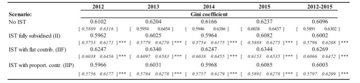
IST reduces significantly income inequality apart from the case in which farmers are required to pay a flat rate contribution to the mutual fund (i.e., each farm pays the

same amount) (scenario IIF). Table3 reports the Gini coefficients calculated without

the IST (baseline) and under the three scenarios of IST application: IST fully subsidized

and IST with flat rate contribution and with proportional contribution (Table1).

Concentration declines when indemnification costs are subsidized fully by the govern-ment and when farms pay proportional contributions. On the other hand, concentration

increases in the flat rate case (Table3). This happens in almost all considered years.

Ac-cording to the ANOVA results, the concentration always differs statistically (at 1%

signifi-cance level) with the IST in place when compared with the“No IST”case (Table3)19.

If farmers are asked to pay contributions that are proportional to their income level, the effect of IST in terms of reducing income concentration is very similar to that

which occurs when it is fully subsidized (Table3)20. On the other hand, in all but two

cases the application of IST with a flat rate contribution causes a significant increase in

income inequality in all considered periods (Table3).

Contribution of direct payments and IST to income equality: results of the Gini decomposition

The Gini decomposition analysis focuses on the case in which farmers pay a contribu-tion that is proporcontribu-tional to their expected incomes because it is the most likely scenario

for its application21. The three considered income sources generate very different

shares of the overall farm income. On average, market income accounts for around

Table 3Effects of the IST on farm income concentration. Gini coefficient without and with the simulated implementation of the IST. Years from 2012 to 2015 and whole period

Note: Numbers in brackets depict 95% confidence intervals

***Difference to the“no insurance”scenario (No IST) is significant at the 1% level

Source: Own elaborations on Italian FADN data

19

Results for the Theil indexes and the 80/20 ratios confirm this finding (Table 7 in the Appendix).

20_{ANOVA results do not allow rejection of the null hypothesis (i.e. concentration levels do not differ}

between IST scenarios) at the 5% level of significance.

21

79% of the farm income, direct payments around 15% and the net financial benefits of

IST 6% (Table4).

As reported by previous analyses, direct payments are relatively more concentrated

than market incomes (Gini coefficientGkin Table4) (Severini et al., 2014a and b).

We find that the net financial benefits of IST are extraordinarily concentrated because of the nature of this tool: it provides indemnifications only to a limited share of the farms each year. In all considered years, the Gini coefficient is higher than unity because the ma-jority of the farms have a negative net financial benefit from the application of IST since they pay contributions without receiving any indemnification. However, when the 4 years reviewed are considered together, there is a marked decline in the number of farms with a negative average net benefit from IST in comparison with the single year cases. Therefore, the concentration of this income source calculated over the whole 4-year period (bottom

panel of Table4) is lower than when calculated on a single year basis.

Table 4Gini decomposition by income sources. All farm sample, years from 2012 to 2015 and whole period

^Assuming that farmers pay contributions proportional to their income to cover 35% of the overall indemnification cost (scenario IIP)

The income concentration-reducing role of IST is driven by a small Gini correlation

(Rk) (Table 4). This means that the financial benefits from IST are not distributed in

favor of high-income farms, given that this income component is only correlated very weakly with the rank of the overall farm income. It is important to note that the net fi-nancial benefits from the application of IST have an even lower Gini correlation than direct payments (i.e., around half that of direct payments).

Based on these latter results, the proportional contribution of the net benefits from the IST to the overall income concentration (Pk) is lower than its share (Sk) (Table4). A similar situation is found for direct payments while the opposite is true for market income.

IST reduces income concentration as shown by the negative elasticity of the fi-nancial benefits it provides. In accordance with the results of El Benni and Finger (2014a), the proportional contribution to income concentration (i.e., Pk) of the in-come generated by IST is substantially lower than that of the other two inin-come

components (Table 4). However, this result is strongly influenced by the fact that

the share of the income derived by IST is far less relevant than that of the other income components.

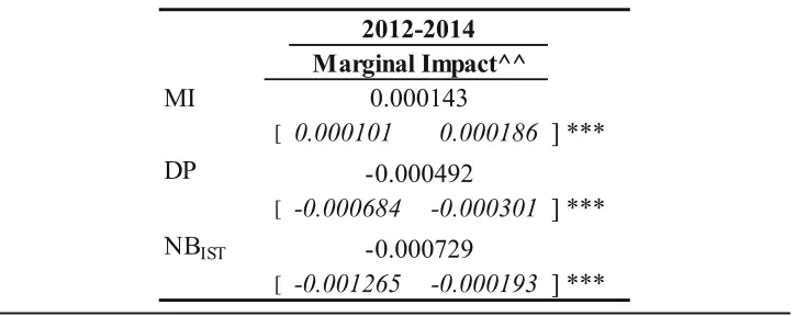
Therefore, to facilitate the comparison, we also derive the marginal contribution of each source of income. This permits a comparison of their effects on income inequality even if these sources represent different shares of the overall income. The marginal impact of IST is significantly different from zero according to

Wilcoxon rank sum tests and more negative than that of direct payments (Table5). This

suggests that IST could indeed play a significant role in reducing income concentration22.

While the extent of the marginal impact of the IST benefits exceeds that of direct payments, the obtained confidence intervals often overlap. Hence, it is not possible to reject the hypothesis of differences of marginal impact of IST from that of direct

payments (Table5).

The analysis has shown that direct payments and IST have a similar income concentration-reducing effect at the margin under the current conditions. However, this may not necessarily be the case when considering a level of direct payments that differs from the one currently in force. To analyze this issue, we first simulate a linear

Table 5Gini decomposition under the scenario of implementation of IST with a contribution proportional to farm income (Scenario IIP). Levels and confidence intervals^ of marginal impact^^ by income source. Years from 2012 to 2015 and whole period

^95% confidence intervals derived from the bootstrap procedure reported in brackets ^^Marginal Impact expressed as impact of an increase of 1000 Euro/farm

MImarket income,DPdirect payments;NBISTnet benefits from IST under the hypothesis of proportional contributions

Source: Own elaborations on Italian FADN data

22_{The results of the Gini decomposition do not change significantly when considering transaction costs equal}

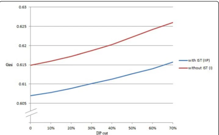
relative cut of direct payment levels and, subsequently, we assess the impact of the application of IST on income concentration. This simulation is performed only under

the assumption that farmers’ contribution to the mutual fund is proportional to their

average income (scenario IIP). As expected, cutting direct payments causes the income

concentration to increase even with the IST in place. Furthermore, the reduction of the

normalized Gini coefficient (Chen et al., 1982) caused by IST has roughly the same

magnitude for all considered levels of direct payments (Fig. 4). However, under the

simulated conditions, IST does partially counteract the effect of cutting direct payments regarding income concentration.

To summarize, results clearly show that IST can reduce income inequality if farmers pay a contribution that is proportional to their income. In contrast, a flat rate contribu-tion increases income inequality, a finding that contrasts with those of Finger and El Benni (2014a) for Swiss agriculture23

Conclusions

In this paper, we provide a multidimensional assessment of the IST by evaluating the possible implications of its implementation in terms of income stabilization,

23

This is probably because of three main reasons. First, the income concentration observed in the baseline case (without IST) is substantially higher in Italy than in Switzerland because the farming population in Italy is very heterogeneous in terms of farm size. According to the 2013 Farm Structural Survey, while the average farm size is around 12 ha of Utilized Agricultural Area, 58% of the Italian farms are smaller than 5 ha while 8% are larger than 30 ha (Eurostat,2013). Second, the application of IST with the flat rate approach (i.e. as used by Finger and El Benni (2014a)) has a negative impact on the income of the many small Italian farms while favoring large farms. Third, the relative reduction of the concentration due to the fully subsidized IST scenario is smaller in Italy than that reported by Finger and El Benni (2014a).

income levels, and income distribution using the example of Italian agriculture. The analysis also addresses the issue of the interdependencies between IST and CAP direct payments by simulating, on an ex ante basis, the implementation of IST under reduced levels of direct payments. We apply the Gini decomposition by income sources, including both direct payments and the net financial benefits derived from IST, to compare the income concentration effects of both policies.

Our results confirm that IST could stabilize farm income significantly. Further-more, our results reveal two additional aspects that seem important from a policy point of view. Firstly, IST increases the average farm income due to the govern-mental support it provides. However, the extent of this increase is moderate and does not suffice to compensate for large reductions in the level of direct pay-ments. Clearly, it is possible that modifications in policy design (e.g., reductions of trigger level and increases of compensation rate) could alter these results.

Sec-ondly, the analysis confirms the findings of Finger and El Benni (2014a) that IST

could reduce income inequality among the farming population. However, the analysis adds to the current debate by showing that the extent of the income concentration reduction effects of both direct payments and IST has the same sign and similar magnitude at the margin. More specifically, both contribute to reductions of income inequality in the farming population.

The analysis has shown that direct payments and IST are expected to interact since they have similar effects on the three considered dimensions of farm income. First, the results of the analysis suggest that in its current form, IST could provide an amount of income support that partially offset cuts in direct payments that may result from the

current debate on the Multiannual Financial Framework for the period 2021–2027

(European Commission,2018; Matthews,2018). Second, a reduction of direct payments

would only cause a negligible increase in the amount of indemnifications that farmers receive from IST. This is in contrast with the hypothesis that IST will gain importance if direct payments levels are reduced.

The analysis does have some limitations that must be kept in mind when seeking to interpret the results correctly and draw sound policy conclusions. It does not apply

be-havioral models and therefore does not allow for the possible effect of IST on farmers’

production choices. The setting of the analysis suggests that its findings focus on the short run effects of IST and refer to a situation where all farmers participate. Future

analyses will be needed to assess possible effects of IST on farmers’behavior, especially

with respect to changes in production and risk management decisions as well as with respect to participation in such a scheme.

Appendix

Table 6Average farm size in terms of farm income (Euro/farm) and utilized agricultural area (ha/ farm) in the sampled farms. Whole sample, and farms grouped by: altimetry regions, types of farming, farm size, and macro-regions of Italy. Balanced sample (year 2015). Mean values and coefficients of variation (CV) within the groups.

^Coefficient of variation

^^According to economic standard output classes (European Commission,2010)

Table 8Gini decomposition by income sources whole period 2012–2014

^Impact of an increase of 1000 Euro/farm

^^Assuming that farmers pay contributions proportional to their income to cover 35% of the overall indemnification cost (IIP)

Source: Own elaborations on Italian FADN data

Table 7Effects of the IST on farm income concentration. Theil and 80/20 ratio. Years from 2012 to 2015 and whole period

Note: Numbers in brackets depict 95% confidence intervals

***Difference to the“no insurance”scenario (No IST) is significant at the 1% level

Source: Own elaborations on Italian FADN data

Table 9Gini decomposition. Marginal Impact by income source derived from the bootstrap

procedure in the whole period 2012–2014^

^95% confidence intervals reported in brackets

^^Marginal impact expressed as impact of an increase of 1000 Euro/farm ***Different from zero at 1% significance

MImarket income,DPdirect payments,NBISTnet benefits from IST under the hypothesis of proportional contributions

Table 10Average annual farm income levels in the whole 2012–2015 period with application of growing levels of transaction costs. Farmers contribution to the mutual fund proportional to their incomes (scenario IIP)

Source: Own elaborations on Italian FADN data

Table 11Gini decomposition by income sources with transaction cost. All farm sample, years from

2012 to 2015, and whole periods 2012–2015 and 2012–2014. Transaction costs set at 20% of the

contribution

^Impact of an increase of 1000 Euro/farm

^^Assuming that farmers pay contributions proportional to their income to cover 35% of the overall indemnification cost (IIP)

Acknowledgements

We would like to thank the CREA-PB for allowing us to use the data on which the analysis has been developed. The views and opinions expressed in this paper are those of the authors and do not necessarily reflect the position of the CREA-PB.

Authors’contributions

SS has made substantial contributions to the conception and design of the analysis and has coordinated the work. GD and RF have made substantial contributions to its design. GD has developed the data analysis and, together with SS and RF, has interpreted the results. SS and GD have drafted the paper that has been substantively revised by RF. All authors have approved the submitted version.

Authors’information

Simone Severini is professor of agricultural economics and policy at Tuscia University, Viterbo (Italy). Giuliano Di Tommaso is collaborating with Tuscia University, Viterbo (Italy).

Robert Finger is professor and head of the Agricultural Economics and Policy Group, at ETH Zurich (Switzerland).

Funding

This research has been developed within the project“Towards SUstainable and REsilient EU FARMing systems” (SURE-Farm). This project has received funds from the European Union_’s Horizon 2020 research and innovation program under grant agreement no. 727520.

Availability of data and materials

The data analyzed in the current study are available from the Consiglio per la ricerca in agricoltura e l’analisi dell_’economia agraria - Politiche e Bioeconomia (CREA-PB) of Rome (Italy) at:http://bancadatirica.crea.gov.it/Default. aspx. Restrictions apply to the availability of these data, which were used under license for the current study and so are not publicly available. Data are however available from the authors upon reasonable request and with permission of CREA-PB.

Competing interests

The authors declare that they have no competing interests.

Author details

1_{Tuscia University, Viterbo, Italy.}2_{Agricultural Economics and Policy Group, ETH Zurich, Zurich, Switzerland.}

Received: 16 January 2019 Accepted: 9 October 2019

References

Bardají I, Garrido A (2016) State of play of risk management tools implemented by member states during the period 2004 -2020: national and European frameworks. Study requested by the European Parliament_’s Committee on Agriculture and Rural Development. Bruxelles.

Cafiero C, Capitanio F, Cioffi A, Coppola A (2007) Risk and crisis management in the Reformed European Agricultural Policy. Canadian Journal of Agricultural Economics/Revue canadienne d'agroeconomie 55:419–441

Castañeda-Vera A, Garrido A (2017) Evaluation of risk management tools for stabilising farm income under CAP 2014-2020. Economía Agraria y Recursos Naturales 17(1):3–23

Chen CN, Tsaur TW, Rhai TS (1982) The Gini coefficient and negative income. Oxford Economic Papers, New Series 34(3):473–478

Ciliberti S, Frascarelli A (2018).The CAP 2013 reform of direct payments: redistributive effects and impacts on farm income concentration in Italy. Agricultural and Food Economics, 2018 6:19

Cordier J, Santeramo F (2018) Mutual funds and the Income Stabilisation Tool in the EU: Retrospect and Prospects. EuroChoices (December 2018)

Dell_’Aquila C, Cimino O (2012) Stabilization of farm income in the new risk management policy of the EU: a preliminary assessment for Italy through FADN data. Paper presented at the 126thEAAE Seminar:“New challenges for EU agricultural sector and rural areas. Which role for public policy?_”. Capri, Italy.

Efron B (1993) An introduction to the bootstrap. Chapman & Hall/CRC, New York

El Benni N, Finger R (2013) The effect of agricultural policy reforms on income inequality in Swiss agriculture_–An analysis for valley, hill and mountain regions. Journal of Policy Modeling 35(4):638–651

El Benni N, Finger R, Mann S (2012) Effects of agricultural policy reforms on income risks in Swiss agriculture. Agricultural Finance Review 72(3):301–324

El Benni N, Finger R, Meuwissen M (2016) Potential effects of the income stabilisation tool (IST) in Swiss agriculture. European Review of Agricultural Economics 43(3):475–502

Enjolras G, Capitanio F, Aubert M, Adinolfi F (2014) Direct payments, crop insurance and the volatility of farm income. Some evidence in France and Italy. New Medit 1:31–40

European Commission (EC) (2009) Income variability and potential cost of income insurance for EU. Directorate-General for Agriculture and Rural Development, Brussels, Belgium

European Commission (EC), 2010. Farm accountancy data network. An A to Z of methodology. Available at:http://ec.europa. eu/agriculture/rica/pdf/site_en.pdf.

European Commission (EC), 2018. A modern budget for a union that protects, empowers and defends. The Multiannual Financial Framework for 2021-2027. COM(2018) 321 final. Brussels, 2.5.2018.

Findeis JL, Reddy VK (1987) Decomposition of income distribution among farm families. Northeastern Journal of Agricultural Economics 16:165–173

Finger R, El Benni N (2014a) A note on the effects of the Income Stabilisation Tool on income inequality in agriculture. Journal of Agricultural Economics 65(3):739–745

Finger R, El Benni N (2014b) Alternative specifications of reference income levels in the income Stabilization Tool. In: Zopounidis C, Kalogeras N, Mattas K, Dijk G, Baourakis G (eds) Agricultural Cooperative Management and Policy. Springer Finger R, Lehmann N (2012) The influence of direct payments on farmers' hail insurance decisions. Agricultural Economics 43(3):343–354 Fresco LO, Poppe KJ (2016) Towards a common agricultural and food policy. Wageningen University & Research

Galán-Martín Á, Pozo C, Guillén-Gosálbez G, Vallejo AA, Esteller LJ (2015) Multi-stage linear programming model for optimizing cropping plan decisions under the new Common Agricultural Policy. Land use policy 48:515–524 Hennessy DA (1998) The production effects of agricultural income support policies under uncertainty. American Journal of

Agricultural Economics 80(1):46–57

Iyer P, Bozzola M, Hirsch S, Meraner M, Finger R (2019) Measuring farmer risk preferences in Europe: a systematic review. Journal of Agricultural Economics. In Press.https://doi.org/10.1111/1477-9552.12325

Keeney M (2000) The distributional impact of direct payments on Irish incomes. Journal of Agricultural Economics 51(2):252–263 Kimura S, Antón J (2011) Farm income stabilization and risk management: some lessons from Agristability Program in Canada.

Paper presented at the International Congress of the European Association of Agricultural Economists. Zurich, Switzerland Lerman RJ, Yitzhaki S (1985) Income inequality effects by income source: a new approach and applications to the U.S. Review

of Economics and Statistics 67:151–156

Liesivaara P, Myyrä S (2016a) The demand for public-private crop insurance and government disaster relief. Journal of Policy Modeling 39:19–34

Liesivaara P, Myyrä S (2016b) Income stabilisation tool and the pig gross margin index for the Finnish pig sector, in 90th Annual Conference. Warwick University. Coventry, UK. No. 236360. Agricultural Economics Society.

Liesivaara P, Myyrä S, Jaakkola A (2012) Feasibility of the Income Stabilisation Tool in Finland. Paper prepared for the 123rd EAAE Seminar Price Volatility and Farm Income Stabilisation. Dublin, Ireland.

Mary S, Santini F, Boulanger P (2013) An ex-ante assessment of CAP Income Stabilisation Payments using a farm household model. Paper presented at the 87th_{Annual Conference of the Agricultural Economics Society, University of Warwick.}

Matthews A (2010) Perspectives on addressing market instability and income risk for farmers, Discussion Paper No. 324/April 2010, Institute for International Integration Studies. Trinity College Dublin, Ireland.

Matthews A (2018) By how much is the CAP budget cut in the Commission’s MFF proposals?. Available on line at:http:// capreform.eu/.

Meuwissen MPM, Assefa T, Van Asseldonk MAPM (2013) Supporting insurance in European agriculture; experience of mutuals in the Netherlands. EuroChoices 12(3):10–16

Meuwissen MPM, Huirne RBM, Skees JR (2003) Income insurance in European agriculture. EuroChoices 2(1):12–17 Meuwissen MPM, Mey YD, Van Asseldonk MAPM (2018) Prospects for agricultural insurance in Europe. Agricultural Finance

Review 78(2):174–182

Meuwissen MPM, Van Asseldonk MAPM, Huirne RBM (2008) Income stabilisation in European agriculture. Wageningen Academic Publishers, Wageningen, The Netherlands

Meuwissen MPM, Van Asseldonk MAPM, Pietola KS, Hardaker JB, Huirne RBM (2011) Income Insurance as a Risk Management Tool After 2013 CAP Reforms? EAAE Congress, Zurich, Switzerland

MIPAAF (Italian Ministry of Agriculture), 2017. Italy - Rural Development Programme (National). Version 5.0. Rome, 10/11/2017. Available at:https://www.reterurale.it/psrn.

Moro D, Sckokai P (2013) The impact of decoupled payments on farm choices: conceptual and methodological challenges. Food Policy 41:28–38https://doi.org/10.1016/j.foodpol.2013.04.001

Payton ME, Greenstone MH, Schenker N (2003) Overlapping confidence intervals or standard error intervals: what do they mean in terms of statistical significance? Journal of Insect Science 3(34):1–6

Pigeon M, Henry de Frahan B, Denuit M (2012) Actuarial evaluation of the EU proposed farm income stabilisation tool. Paper prepared for the 123rd EAAE Seminar Price Volatility and Farm Income Stabilisation, 23–24 February. Dublin, Ireland. Pyatt G, Chen C, Fei J (1980) The distribution of income by factor components. Quarterly Journal of Economics 95:451–473 Scheffé H (1959) The analysis of variance. Wiley, New York

Severini S, Biagini L, Finger R (2018) The design of the Income Stabilization Tool in Italy: balancing risk pooling, risk reduction and distribution of policy benefits. Journal of Policy Modeling.https://doi.org/10.1016/j.jpolmod.2018.03.003

Severini S, Tantari A, Di Tommaso G (2016a) The instability of farm income. Empirical evidences on aggregation bias and heterogeneity among farm groups. Bio-based and Applied Economics 5(1):63–81

Severini S, Tantari A, Di Tommaso G (2016b) Do CAP direct payments stabilise farm income? Empirical evidences from a constant sample of Italian farms. Agricultural and Food Economics 4(6):1–17

Shields DA (2015) Federal crop insurance: background. Congressional Research Service. Report, Washington DC, pp 7–5700 Stark O, Taylor JE, Yitzhaki S (1986) Remittances and inequality. The Economic Journal 96:722–740

Trestini S, Giampietri E (2018). Re-adjusting risk management within the CAP: evidences on the implementation of the Income Stabilisation Tool in Italy. In: Wigier M, Kowalski A (Eds) (2018). The Common Agricultural Policy of the European Union–the present and the future EU Member States point of view. Institute of agricultural and food economics national research institute. Warsaw, Poland.

Trestini S, Giampietri E, Boatto V (2017). Toward the implementation of the Income Stabilization Tool: an analysis of factors affecting the probability of farm income losses in Italy. New Medit N. 4/2017: 24-30.

Trestini S, Szathvary T, Pomarici E, Boatto V (2018) Assessing the risk profile of dairy farms: application of the Income Stabilisation Tool in Italy. Agricultural Finance Review 78(2):195–208

Turvey CG (2012) Whole Farm Income Insurance. Journal of Risk and Insurance 79:515–540

Publisher’s Note