Vol.6 (2016) No. 5
ISSN: 2088-5334
Binary Particle Swarm Optimization Structure Selection of
Nonlinear Autoregressive Moving Average with Exogenous Inputs
(NARMAX) Model of a Flexible Robot Arm
Ihsan Mohd Yassin
#1, Azlee Zabidi
#2, Megat Syahirul Amin Megat Ali
#3, Nooritawati Md Tahir
#4, Husna
Zainol Abidin
#6,
Zairi Ismael Rizman
*7#
Faculty of Electrical Engineering, Universiti Teknologi MARA, 40450 Shah Alam, Selangor, Malaysia E-mail: [email protected], [email protected], [email protected], [email protected],
6
*Faculty of Electrical Engineering, Universiti Teknologi MARA, 23000 Dungun, Terengganu, Malaysia
E-mail: [email protected]
Abstract
—
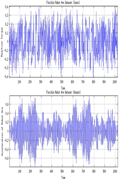
The Nonlinear Auto-Regressive Moving Average with Exogenous Inputs (NARMAX) model is a powerful, efficient and unified representation of a variety of nonlinear models. The model’s construction involves structure selection and parameter estimation, which can be simultaneously performed using the established Orthogonal Least Squares (OLS) algorithm. However, several criticisms have been directed towards OLS for its tendency to select excessive or sub-optimal terms leading to nonparsimonious models. This paper proposes the application of the Binary Particle Swarm Optimization (BPSO) algorithm for structure selection of NARMAX models. The selection process searches for the optimal structure using binary bits to accept or reject the terms to form the reduced regressor matrix. Construction of the model is done by first estimating the NARX model, then continues with the estimation of the MA model based on the residuals produced by NARX. One Step Ahead (OSA) prediction, Mean Squared Error (MSE) and residual histogram analysis were performed to validate the model. The proposed optimization algorithm was tested on the Flexible Robot Arm (FRA) dataset. Results show the success of BPSO structure selection for NARMAX when applied to the FRA dataset. The final NARMAX model combines the NARX and MA models to produce a model with improved predictive ability compared to the NARX model.Keywords— system identification, NARMAX, structure selection, particle swarm optimization
I. INTRODUCTION
System Identification (SI) is a control engineering discipline concerned with the inference of mathematical models from dynamic systems based on their input and/or output measurements [1]-[5]. It is fundamental for system control, analysis and design where the resulting representation of the system can be used for understanding the properties of the system as well as prediction of the system’s future behavior under given inputs and/or outputs [6].
SI is a significant research area in the field of control and modeling due to its ability to represent and quantify variable interactions in complex systems. Several applications of SI in literature are for understanding of complex natural phenomena [7]-[11], model-based design of control engineering applications [12]-[16] and project monitoring and planning [17]-[19].
Many SI models exist. Among them, the Nonlinear Auto-Regressive Moving Average with Exogenous Inputs (NARMAX) [20] model is a powerful, efficient and unified representations of a variety of nonlinear models [21]-[30]. A rich literature is available regarding its success in various electrical, mechanical, medical and biological applications [31]-[33].
Simultaneous structure selection and parameter estimation of NARMAX and derivative models are achievable through the Orthogonal Least Squares (OLS) algorithm [34], [35]. The OLS algorithm has since been widely accepted as a standard [36] and has been used in many works [37]-[43] due to its simplicity, accuracy and effectiveness.
selected incorrect terms when the data is contaminated by certain noise sequences or when the system input is poorly designed. The suboptimal selection of regressor terms leads to models that are inaccurate or non-parsimonious in nature.
This study proposes the Binary Particle Swarm Optimization (BPSO) algorithm to perform structure selection for the NARMAX. Using the BPSO approach, the structure selection problem is considered as a binary optimization problem to minimize an objective function. Unlike OLS (which uses ERR to rank regressors that significantly reduce the error variance in order to select the best regressors for the model), no preference is given to any regressor. Rather, BPSO treats the regressors equally (all regressors have an equal chance of being selected) and the model structure is defined towards minimizing certain objective criteria.
II. THE NARMAXMODEL
The NARMAX model output is dependent on its past inputs, outputs and residuals [44], [45]. Construction of the model can employ various methods such as polynomials [46]-[49], Multilayer Perceptrons (MLP) [50]-[52] and Wavelet ANNs (WNN) [53], [54] although the polynomial approach is the only method that can explicitly define the relationship between the input/output data.
The identification method for NARMAX is performed in three steps. Structure selection is performed to detect the underlying structure of a dataset. This is followed by parameter estimation to optimize some objective function (typically involving the difference between the identified model and the actual dataset). The NARMAX model recursively adds residual terms to the Nonlinear Auto-Regressive with Exogenous Inputs (NARX) model to eliminate the bias and improve the model prediction capability [55]. Structure selection and parameter estimation for NARMAX are recursively repeated on the residual set until a satisfactory model is obtained. Finally, the model is validated to ensure that it is acceptable.
A major advantage of NARMAX and its derivatives is that it provides physically interpretable results that can be compared directly, thus providing a way to validate and enhance analytical models where first principle models lack the completeness because of assumptions and omissions during derivations. Furthermore, among all the models studied, it is the only model that embeds the dynamics of nonlinearities directly into the model [56]. Other advantages include model representativeness [57], flexible model structure, reliability over a broad range of applications as well as reasonable parameter count and computational costs (for reasonably-sized model structures) [58].
III.PARTICLE SWARM OPTIMIZATION AND ITS APPLICATION FOR NARMAX STRUCTURE SELECTION
A. Particle Swarm Optimization
Optimization is generally defined as a task to search for an optimal set of solutions for a parameter-dependent problem, typically by minimizing a cost function related to the problem [59].
The PSO algorithm is a global stochastic optimization algorithm based on the swarming behavior of animals in
nature. The algorithm defines particles as agents responsible for searching the solution space. The movement of particles is directed by the particles’ best individual achievement, as well as the best swarm achievement [60], [61]. The iterative search process continues until the objective is met or the number of iterations is exhausted. Among the advantages of PSO are:
1. Usage of simple mathematical operators makes it easy to implement [62]-[69].
2. It is computationally inexpensive and fast compared to other more complex optimization algorithms [70]-[73]. 3. It has a successful track record in solving complex
optimization problems [74], [75].
4. It is versatile: can be easily adapted to solve continuous, binary or discrete problems. No requirement of gradient information thus can be used for a wide range of problems otherwise non-optimizable by gradient-based algorithms.
5. It requires a minimum amount of parameter adjustments.
6. It is robust in solving complex optimization problem [76].
7. It can be implemented in a true parallel fashion [77].
B. Binary PSO for Structure Selection
The polynomial representation of the NARMAX model for a given input–output series is:
= ∑ + (1)
where is the number of terms in the polynomial expansion, is the -th regression term with = 1, and is the -th regression parameter. is formed by a combination of input, output and residual terms. In matrix form, identification involves the formulation and solution of the Least Squares (LS) problem:
+ = (2)
where is a × regressor matrix, is a × 1 coefficient vector, is the × 1 vector of actual observations, is arranged such that its columns represent the lagged regressors and is the white noise residuals.
The NARMAX model construction is performed in two steps, namely model structure selection and parameter estimation. Structure selection involves selecting which columns in that best describes the observations, . After a subset of has been selected, the parameter estimation step estimates the parameters of the function ∎ that gives the best fit for (Equation (3)):
= − 1 , − 2 , … , − , ! −
" , ! − "− 1 , … , ! − "− # , − 1 ,
− 2 , … , − $ % + % (3)
The use of BPSO for model structure selection is described. Consider the identification problem in Equation (2) defined in an LS matrix form. The BPSO algorithm defines a binary string of length 1 × so that each column in has a bit assigned to it. A value of 1 indicates that the column is included in the reduced regressor matrix ( & , while the value of 0 indicates that the regressor column is ignored. The initial binary string is a predefined parameter prior to optimization.
The BPSO algorithm is directed by two equations, namely the velocity update equation and the position update equation. The velocity update equation is given by [78]:
'( = ) '( + * +,-.− /( × 01 2 + *3 4+,-.− /( × 01 23 (4)
Next, the value of '( is then used to modify the particle positions, /( :
/( = /( + '( (1)
where '( = particle velocity, /( = particle position, +,-. = particle’s best fitness so far, 4+,-. = best solution achieved by the swarm so far, * = cognition learning rate, *3 = social learning rate and 01 2 , 01 23 = uniformly-distributed random numbers between 0 and 1.
During optimization, each particle in the swarm carries a 1 × vector of solutions, 5( . This vector contains the change in probability defined in Equation (6):
67 8 07 9 = 1 7 5( : 0.5
67 8 07 9 = 0 7 x( ? 0.5 (2)
During optimization, the 5( values change and alter which regressor column is selected. The linear least squares solution ( &) for the reduced regressor matrix ( &) can then be estimated using the QR factorization method:
& &+ = (3)
&= @&A& (4)
9&= @&B (5)
A& &= 9& (6)
Alternatively, methods such as the Newton-Rhapson algorithm can also be used [79].
IV.MATERIAL AND METHODS
A. Experiment Hardware
All experiments were performed on a personal computer with 3.10GHz Intel Xeon E3-1220 v3 microprocessor and 4GB RAM. The operating system was Linux Mint XFCE version 17.1 with MATLAB 2014a as the development platform.
B. Methodology
A general overview of the methodology is presented in Fig. 1, and a description of each process is presented in the following sections.
Fig. 1 Structure selection experiment overview
Pre-processing is an important step for data conditioning prior to identification. In experiments conducted in this work, the division for the Flexible Robot Arm (FRA) dataset was 50% for training set and 50% for testing set based on the recommendation by [51].
C. Create Regressor Matrices
This process constructs the full regressor matrix ( ) from which BPSO can choose candidate terms to form the reduced regressor matrix, &. After the first-level structure selection process, a second-level MA structure selection was performed recursively using lagged residual terms.
D. Find Optimal Parameters for Structure Selection
After the regressors matrices have been constructed, BPSO was applied to evaluate the candidate structures and determine the best structure.
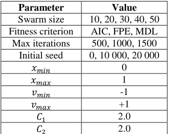
BPSO convergence depends on several parameters, which need to be tested to determine their optimal values. Therefore, experiments were done by performing optimization under various combinations of parameters swarm size, maximum iterations and several random seeds. Table 1 shows the tested parameter values.
TABLE I
BPSO PARAMETER SETTINGS FOR STRUCTURE SELECTION EXPERIMENTS
Parameter Value
Swarm size 10, 20, 30, 40, 50 Fitness criterion AIC, FPE, MDL
Max iterations 500, 1000, 1500 Initial seed 0, 10 000, 20 000
5 ( 0
5 CD 1
E ( -1
E CD +1
* 2.0
*3 2.0
The choice of swarm size and maximum iterations were based on preliminary test to balance between speed and solution quality. These values were considered optimal given the limited computational hardware resources available.
Three random seeds were chosen for the Mersenne-Twister Algorithm. The seeds are used to generate traceable random numbers to ensure repeatability of experiments performed. The values are arbitrary, but important to ensure that the experiments are repeatable.
The values of particle minimum value (5 ( and particle maximum value (5 CD were set to 0 and 1 respectively. They are within the range of probability values for a bit change to occur. E ( and E CD represent the movement range of the particles. Since the value of 5( is between the range of 0 and 1 (based on 5 ( and 5 CD), the values of E ( and E CD were set to -1 (when 5( moves from 1 to 0) and +1 (when 5( moves from 0 to 1) respectively. The values of * and *3 were both set to 2.0. This parameter is well-accepted as optimal based on literature [80].
The optimization is guided by Akaike Information Criterion (AIC), Final Prediction Error (FPE) and Model Descriptor Length (MDL) [81] criteria:
'FGH = I1 + 2JK '2 LMMN , OL (7)
'PQR = S1 + lU9V J LW 'LMMN , OL (8)
'XYN= Z [\]
^\]_ 'LMMN , OL (9)
where 2 is the number of estimated parameters, J is the number of data points. 'LMMN , OL is the Normalized Sum
Squared Error (NSSE) of the model residuals with respect to the model parameters, :
'LMMN , OL =
3L∑L. 3 , (10)
Theoretically, the values of'FGH , 'PQR and 'XYN are minimum when 'LMMN , OL = 0 at which 2 is irrelevant. However, this never happens in real modeling scenarios thus the value of 2 must be taken into account. With the inclusion of 2, the values of 'FGH, 'PQR and 'XYN are minimum when 'LMMN , OL → 0 and 2 → 1. Models with the lowest 'FGH, 'PQR and 'XYN scores obey the principle of parsimony as the least amount of parameters were required to provide the best fit for the data.
E. Model Validation and Analysis
After structure selection has been performed, the resulting candidate models need to be validated and analyzed to determine the best model. One Step Ahead (OSA) and residual tests were performed to select the best model that fulfills the validation criteria. Several tests, namely the OSA prediction, Mean Squared Error (MSE) and residual histogram analysis were performed to validate the model.
OSA is a test that measures the ability of a model to predict future values based on its previous data. It takes the form of [82]:
a t = 9a c (11)
where 9a is the estimated nonlinear model, and c are the regressors. Representation of c for the NARMAX model is shown in Equation (16):
c = [ − 1 , − 2 , … , − , ! − "− 1 , ! − "− 2 , … , ! − "− # , − 1 , − 2 , … , − $ %
(12)
MSE is a standard method for testing the magnitude of the residuals for regression and model fitting problems. The MSE equation for a residual vector of length is given by:
efg = ∑L( ( ⁄J (13)
where ( is the observed value and a( is the estimated value at point 7. As MSE values are calculated from the magnitude of the residuals, low values indicate a good model fit. The ideal case for MSE is zero (when (− a(= 0, 7 = 1, 2, … , ). However, this rarely happens in actual modeling scenarios and a sufficiently small value is acceptable.
The third test is the histogram test to measure the whiteness of the residuals. A histogram is a graphical method to present a distribution summary of a univariate data set [83]. It is drawn by segmenting the data into equal-sized bins (classes), then plotting the frequencies of data appearing in each bin. The horizontal axis of the histogram plot shows the bins, while the vertical axis depicts the data point frequencies.
system has been fully captured by the SI model, leaving only un-modeled white noise as the residuals. The purpose of histogram analysis is used to view the distribution of the residuals. The histogram exhibits white noise as a Gaussian distribution, with symmetric bell-shaped distribution with most of the frequency counts grouped in the middle and tapering off at both tails [83].
V. RESULTS AND DISCUSSION
A. NARX Modeling Results
The NARX model produced by BPSO selected five terms of the generated following equation to represent the FRA system:
= 0.0203! − 2 + 3.1204 − 1 − 4.3509 − 2 + 3.0420 − 3 − 0.9453 − 4 +
(14)
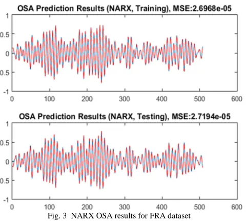
The OSA plots for the training and testing sets were generated based on Equation (18) (Fig. 3). The red line indicates the predicted output of the model, while the blue line indicates the actual FRA system output. Based on the low MSE between the system output and the predicted model, it was concluded that the model managed to represent the system well.
Fig. 3 NARX OSA results for FRA dataset
However, another important criteria of system identification is the whiteness of the residuals. This is because non-random residuals indicate model bias as not all dynamics in the original system is sufficiently captured by the model. As shown in the histogram plots in Fig. 4, the distribution appears as a Gaussian indicating the residuals are random similar to white noise. The addition of the Moving Average (MA) terms described in the next section is presented to improve the prediction accuracy of the model.
B. MA Modeling Results
The second experiment produced the MA model presented here. The result of the NARX residuals is being fed back to the model in order to improve its prediction. The MA model obtained is defined in Equation (19):
= −2.7440 − 2 + 2.2573 − 1 + 1.8697 − 3 − 4.0561 − 2 − 4 − 0.6180 − 4 + 0.0501 − 1 ! − 2 − 0.4490 − 3 ! − 2 + 0.6687 − 3 ! − 3 − 0.5049 − 3 ! − 4 − 0.0901 − 4 − 2 + 3
(15)
Fig. 4 Residual histogram of the FRA NARX model
Fig. 5 MA OSA results for FRA dataset
Fig. 7 NARMAX OSA result for FRA dataset
The OSA results of the MA model are presented in Fig. 5. The selection of higher-order terms in Equation (21) (lags above 2) indicates the complexity of the un-modeled dynamics still present in the system. The OSA prediction of the MA model indicates that the model managed to approximate the residuals well. The MA results were finally combined back into the NARX model to form the final NARMAX model (described in the next section).
C. NARMAX Modeling Results
The final NARMAX model was constructed by combining the results from the NARX and MA models (Equation 20):
y t = 0.0203u t − 2 + 3.1204y t − 1 − 4.3509y t − 2 + 3.0420y t − 3 − 0.9453y t − 4 − 2.7440 t − 2 + 2.2573ε t − 1 +
1.8697ε t − 3 − 4.0561ε t − 2 ε t − 4 − 0.6180ε t − 4 + 0.0501ε t − 1 u t − 2 − 0.4490ε t − 3 u t − 2 + 0.6687ε t − 3 u t − 3 − 0.5049ε t − 3 u t − 4 − 0.0901ε t − 4 y t − 2 + ε3 t
(16)
The OSA for the NARMAX model and a histogram of residuals are shown in Fig. 6 and Fig. 7 respectively. It can be seen that the introduction of the MA terms had a positive effect on the model as the MSE was smaller compared to NARX. The model was also considered valid as the residual histogram also shows a Gaussian distribution, which signifies that the residuals are randomly distributed.
VI.CONCLUSIONS
A BPSO-based structure selection method for NARMAX model was successfully implemented in this paper. The selection process searches for the optimal structure using binary bits to accept or reject the terms to form the reduced regressor matrix. Construction of the model is done by first estimating the NARX model, then continues with the
estimation of the MA model based on the residuals produced by NARX. The final NARMAX model combines the NARX and MA models to produce a model with improved predictive ability compared to the NARX model.
ACKNOWLEDGMENT
The authors would like to express their gratitude to Universiti Teknologi MARA, Malaysia for equipment and infrastructure support for the research.
REFERENCES
[1] H. V. H. Ayala, D. Habineza, M. Rakotondrabe, C. E. Klein and L. S. Coelho, "Nonlinear black-box system identification through neural networks of a hysteretic piezoelectric robotic micromanipulator,"
IFAC-PapersOnLine, vol. 48, pp. 409-414, Dec. 2015.
[2] G. Zhang, X. Zhang and H. Pang, "Multi-innovation auto-constructed least squares identification for 4 DOF ship manoeuvring modelling with full-scale trial data," ISA Transactions, vol. 58, pp. 186-195, Sep. 2015.
[3] M. A. Golkar and R. E. Kearney, "Closed-loop identification of the dynamic relation between surface EMG and torque at the human ankle," IFAC-PapersOnLine, vol. 48, pp. 263-268, Dec. 2015. [4] O. A. Dahunsi and J. O. Pedro, "Nonlinear active vehicle suspension
controller design using PID reference tracking," Journal of the
Institute of Industrial Applications Engineers, vol. 3, pp. 111-120, Jul.
2015.
[5] A. D. Wiens and O. T. Inan, "A novel system identification technique for improved wearable hemodynamics assessment," IEEE Transactions on Biomedical Engineering, vol. 62, pp. 1345-1354,
May 2015.
[6] C. Dash, S. Kumar, A. K. Behera, S. Dehuri and S. B. Cho, Radial basis function neural networks: A topical state-of-the-art survey,"
Open Computer Science, vol. 6, pp. 33-63, 2016.
[7] D. Engelhart, T. A. Boonstra, R. G. K. M. Aarts, A. C. Schouten and H. van der Kooij, "Comparison of closed-loop system identification techniques to quantify multi-joint human balance control," Annual
Reviews in Control, vol. 41, pp. 58-70, Dec. 2016.
[8] H. M. R. Ugalde, J. C. Carmona, J. Reyes-Reyes, V. M. Alvarado and J. Mantilla, "Computational cost improvement of neural network models in black box nonlinear system identification,"
Neurocomputing, vol. 166, pp. 96-108, Oct. 2015.
[9] A. Joosten, T. Huynh, K. Suehiro, C. Canales, M. Cannesson J. and Rinehart, "Goal-Directed fluid therapy with closed-loop assistance during moderate risk surgery using noninvasive cardiac output monitoring: A pilot study, British Journal of Anaesthesia, vol. 114, pp. 886-892, Jun. 2015.
[10] H. A. Moreno, H. V. Gupta, D. D. White and D. A. Sampson, "Modeling the distributed effects of forest thinning on the long-term water balance and streamflow extremes for a semi-arid basin in the southwestern US," Hydrology and Earth System Sciences, vol. 20, pp. 1241-1267, Mar. 2016.
[11] J. Teh and I. Cotton, "Critical span identification model for dynamic thermal rating system placement," IET Generation, Transmission and
Distribution, vol. 9, pp. 2644-2652, Dec. 2015.
[12] J. Fei and M. Xin, "Adaptive fuzzy sliding mode control of MEMS gyroscope sensor using fuzzy switching approach," Journal of
Dynamic Systems, Measurement, and Control, vol. 137, pp.
051002-1 - 05051002-1002-7, May 20051002-15.
[13] L. P. Perera, P. Oliveira and C. G. Soares, "System identification of nonlinear vessel steering," Journal of Offshore Mechanics and Arctic
Engineering, vol. 137, pp. 031302, Jun. 2015.
[14] R. Potluri and A. K. Singh, "Path-tracking control of an autonomous 4WS4WD electric vehicle using its natural feedback loops," IEEE
Transactions on Control Systems Technology, vol. 23, pp. 2053-2062,
Sep. 2015.
[15] W. Fang, J. Sun, X. Wu and V. Palade, "Adaptive Web QoS controller based on online system identification using quantum-behaved particle swarm optimization," Soft Computing, vol. 19, pp. 1715-1725, Jun. 2015.
[16] E. Kang, S. Hong and M. Sunwoo, "Idle speed controller based on active disturbance rejection control in diesel engines," International
[17] D. Zhu, J. Guo, C. Cho, Y. Wang and K. M. Lee, "Wireless mobile sensor network for the system identification of a space frame bridge,"
IEEE/ASME Transactions on Mechatronics, vol. 17, pp. 499-507,
Jun. 2012.
[18] L. YuMin, T. DaZhen, X. Hao and T. Shu, "Productivity matching and quantitative prediction of coalbed methane wells based on BP neural network," Science China Technological Sciences, vol. 54, pp. 1281-1286, May 2011.
[19] J. W. Pierre, N. Zhou, F. K. Tuffner, J. F. Hauer, D. J. Trudnowski and W. A. Mittelstadt, "Probing signal design for power system identification," IEEE Transactions on Power Systems, vol. 25, pp. 835-843, May 2010.
[20] I. J. Leontaritis and S.A. Billings, "Input-output parametric models for nonlinear systems," International Journal of Control, vol. 41, pp. 311-341, Feb. 1985.
[21] E. M. A. M. Mendes and S. A. Billings, "An alternative solution to the model structure selection problem," IEEE Transactions on
Systems, Man and Cybernetics-Part A: Systems and Humans, vol. 31,
pp. 597-608, 2001.
[22] L. A. Aguirre, G. G. Rodrigues and E. M. Mendes, "Nonlinear identification and cluster analysis of chaotic attractors from a real implementation of Chua's circuit," International Journal of
Bifurcation and Chaos, vol. 7, pp. 1411-1423, Jun. 1997.
[23] N. Chiras, C. Evans and D. Rees, "Nonlinear gas turbine modeling using NARMAX structures," IEEE Transactions on Instrumentation
and Measurement, vol. 50, pp. 893-898, Aug. 2001.
[24] M. Vallverdu, M. J. Korenberg and P. Caminal, "Model identification of the neural control of the cardiovascular system using NARMAX models," in Proc. CinC'91, 1991, p. 585-588.
[25] S. L. Kukreja, H. L. Galiana and R. E. Kearney, "NARMAX representation and identification of ankle dynamics," IEEE
Transactions on Biomedical Engineering, vol. 50, pp. 70-81, Jan.
2003.
[26] S. L. Kukreja, R. E. Kearney and H. L. Galiana, "A least squares parameter estimation algorithm for switched Hammerstein systems with applications to the VOR," IEEE Transactions on Biomedical
Engineering, vol. 52, pp. 431-444, Mar. 2005.
[27] N. A. Rahim, M. N. Taib and M. I. Yusof, "Nonlinear system identification for a DC motor using NARMAX approach," in Proc.
AsiaSense'03, 2003, p. 305-311.
[28] K. K. Ahn and H. P. H. Anh, "Inverse double NARX fuzzy modeling for system identification," IEEE/ASME Transactions on Mechatronics, vol. 15, pp. 136-148, Feb. 2010.
[29] Y. Cheng, L. Wang, M. Yu and J. Hu, "An efficient identification scheme for a nonlinear polynomial NARX model," Artificial Life
Robotics, vol. 16, pp. 70-73, Jun. 2011.
[30] M. Shafiq and N. R. Butt, "Utilizing higher-order neural networks in u-model based controllers for stable nonlinear plants," International Journal of Control, Automation and Systems, vol. 9, pp. 489-496, Jun. 2011.
[31] Z. H. Chen and Y. Q. Ni, "On-board identification and control performance verification of an MR damper incorporated with structure," Journal of Intelligent Material Systems and Structures, vol. 22, pp. 1551-1565, Sep. 2011.
[32] B. H. G. Barbosa, L. A. Aguirre, C. B. Martinez and A. P. Braga, "Black and gray-box identification of a hydraulic pumping system,"
IEEE Transactions on Control Systems Technology, vol. 19, pp.
398-406, Mar. 2011.
[33] B. Cosenza, "Development of a neural network for glucose concentration prevision in patients affected by type 1 diabetes,"
Bioprocess and Biosystems Engineering, vol. 35, pp. 1249-1249,
2012.
[34] S. A. Billings, M. Korenberg and S. Chen, "Identification of nonlinear output-affine systems using an orthogonal least-squares algorithm," International Journal of Systems Science, vol. 19, pp. 1559-1568, Jan. 1988.
[35] L. Piroddi, "Simulation error minimisation methods for NARX model identification," International Journal of Modelling, Identification and Control, vol. 3, pp. 392-403, Jan. 2008.
[36] H. L. Wei and S. A. Billings, "Model structure selection using an integrated forward orthogonal search algorithm assisted by squared correlation and mutual information," International Journal of
Modeling, Identification and Control, vol. 3, pp. 341-356, Jan. 2008.
[37] H. L. Wei and S. A. Billings, "An adaptive orthogonal search algorithm for model subset selection and non-linear system identification," International Journal of Control, vol. 81, pp. 714-724, May 2008.
[38] L. A. Aguirre and E. C. Furtado, "Building dynamical models from data and prior knowledge: The case of the first period-doubling bifurcation," Physical Review, vol. 76, pp. 046219-1 - 046219-12, Oct. 2007.
[39] D. G. Dimogianopoulos, J. D. Hios and S. D. Fassois, "FDI for aircraft systems using stochastic pooled-NARMAX representations: Design and assessment," IEEE Transactions on Control Systems
Technology, vol. 17, pp. 138513-138597, 2009.
[40] W. U. Yunna and S. I. Zhaomin, "Application of radial basis function neural network based on ant colony algorithm in credit evaluation of real estate enterprises," in Proc. ICMSE'08, 2008, p. 1322-1329. [41] Y. W. Wong, K. P. Seng and L. M. Ang, "Radial basis function
neural network with incremental learning for face recognition," IEEE
Transactions on Systems, Man and Cybernetics-Part B: Cybernetics,
vol. 41, pp. 940-949, Aug. 2011.
[42] M. J. Er, F. Liu and M. B. Li, "Self-constructing fuzzy neural networks with extended Kalman filter," International Journal of
Fuzzy Systems, vol. 12, pp. 66-72, Mar. 2010.
[43] C. C. Liao, "Enhanced RBF network for recognizing noise-riding power quality events," IEEE Transactions on Instrumentation and
Measurement, vol. 59, pp. 1550-1561, Jun. 2010.
[44] L. Piroddi and M. Lovera, "NARX model identification with error filtering," in Proc. IFAC'08, 2008, p. 2726-2731.
[45] M. A. Balikhin, R. J. Boynton, S. N. Walker, J. E. Borovsky, S. A. Billings and H. L. Wei, "Using the NARMAX approach to model the evolution of energetic electrons fluxes at geostationary orbit,"
Geophysical Research Letters, vol. 38, pp. 1-5, Sep. 2011.
[46] S. R. Anderson, N. F. Lepora, J. Porrill and P. Dean, "Nonlinear dynamic modeling of isometric force production in primate eye muscle," IEEE Transactions on Biomedical Engineering, vol. 57, pp. 1554-1567, Jul. 2010.
[47] B. A. Amisigo, N. v. d. Giesen, C. Rogers, W. E. I. Andah and J. Friesen, "Monthly streamflow prediction in the Volta basin of West Africa: A SISO NARMAX polynomial modelling," Physics and
Chemistry of the Earth, vol. 33, pp. 141-150, Dec. 2007.
[48] S. Chen, S. A. Billings and W. Luo, "Orthogonal least squares methods and their application to non-linear system identification,"
International Journal of Control, vol. 50, pp. 1873-1896, Nov. 1989.
[49] S. A. Billings and S. Chen, "Extended model set, global data and threshold model identification of severely non-linear systems,"
International Journal of Control, vol. 50, pp. 1897-1923, Nov. 1989.
[50] N. A. Rahim, "The design of a non-linear autoregressive moving average with exegenous input (NARMAX) for a DC motor," Master thesis, Universiti Teknologi MARA, Selangor, Malaysia, 2004. [51] M. H. F. Rahiman, "System identification of essential oil extraction
system," Phd thesis, Universiti Teknologi MARA, Selangor, Malaysia, 2008.
[52] M. Norgaard, O. Ravn, N. K. Poulsen and L. K. Hansen, Neural
Networks for Modeling and Control of Dynamic Systems: A Practitioner's Handbook (Advanced Textbooks in Control and Signal Processing), London, UK: Springer, 2013.
[53] H. Wang, Y. Shen, T. Huang and Z. Zeng, Nonlinear System
Identification Based on Recurrent Wavelet Neural Network, ser.
Advances in Soft Computing, H. Wang, Y. Shen, T. Huang and Z. Zeng, Eds. London, UK: Springer, 2009, pp. 517-525.
[54] H. L. Wei and S. A. Billings, "A new class of wavelet networks for nonlinear system identification," IEEE Transactions on Neural
Networks, vol. 16, pp. 862-874, Jul. 2005.
[55] L. A. Aguirre and C. Letellier, "Modeling nonlinear dynamics and chaos: A review," Mathematical Problems in Engineering, vol. 2009, pp. 1-35, Jun. 2009.
[56] D. Spina, B. G. Lamonaca, M. Nicoletti and M. Dolce, "Structural monitoring by the Italian Department of Civil Protection and the case of 2009 Abruzzo seismic sequence," Bull Earthquake Engineering, vol. 9, pp. 325-346, Feb. 2011.
[57] S. Chatterjee, S. Nigam, J. B. Singh and L. N. Upadhyaya, "Software fault prediction using nonlinear autoregressive with exogenous inputs (NARX) network," Applied Intelligence, vol. 37, pp. 121-129, Jul. 2012.
[58] R. Amrit and P. Saha, "Stochastic identification of bioreactor process exhibiting input multiplicity," Bioprocess and Biosystems Engineering, vol. 30, pp. 165-172, May 2007.
[59] M. Yuanbin, "Particle swarm optimization for cylinder helical gearmulti-objective design problems," Applied Mechanics and
Materials, vol. 109, pp. 216-221, 2012.
perturbation and mixed stochastic–deterministic algorithms," IEEE
Transactions on Industrial Electronics, vol. 58, pp. 486-493, Feb.
2011.
[61] Y. Liu, Z. Zhang and Z. Liu, "Customized configuration for hierarchical products: Component clustering and optimization with PSO," International Journal of Advanced Manufacturing Technology, vol. 57, pp. 1223-1233, Dec. 2011.
[62] M. Han, J. Fan and J. Wang, "A Dynamic feedforward neural network based on Gaussian particle swarm optimization and its application for predictive control," IEEE Transactions on Neural
Networks, vol. 22, pp. 1457-1468, Sep. 2011.
[63] S. Karol and V. Mangat, "Use of particle swarm optimization in hybrid intelligent systems," Journal of Information and Operations
Management, vol. 3, pp. 293-296, Jan. 2012.
[64] A. El Dor, M. Clerc and P. Siarry, "A multi-swarm PSO using charged particles in a partitioned search space for continuous optimization," Computational Optimization and Applications, vol. 53, pp. 271-295, Sep. 2012.
[65] W. A. Yang, Y. Guo and W. H. Liao, "Optimization of multi-pass face milling using a fuzzy particle swarm optimization algorithm,"
International Journal of Advanced Manufacturing Technology, vol.
54, pp. 45-57, Apr. 2011.
[66] T. Yu-Bo and X. Zhi-Bin, Particle-Swarm-Optimization-Based
Selective Neural Network Ensemble and Its Application to Modeling Resonant Frequency of Microstrip Antenna, ser. Microstrip Antennas.
N. Nasimuddin, Ed. Rijeka, Croatia: In Tech Open Access Publisher, 2011, pp. 69-82.
[67] G. Folino and C. Mastorianni, "Special issue: Bio-inspired optimization techniques for high performance computing," New
Generation Computing, vol. 29, pp. 125-128, Apr. 2011.
[68] C. N. Ko, "Identification of non-linear systems using radial basis function neural networks with time-varying learning algorithm," IET
Signal Processing, vol. 6, pp. 91-98, Apr. 2012.
[69] A. M. Moussa, M. E. Gammal, A. a. Ghazala and A. I. Attia, "An improved particle swarm optimization technique for solving the unit commitment problem," Online Journal of Power and Energy
Engineering, vol. 2, pp. 217-222, 2011.
[70] X. Na, H. Dong, Z. GuoFu, J. JianGuo and V. Khong, "Study on attitude determination based on discrete particle swarm optimization," Science China Technological Sciences, vol. 53, pp. 3397-3403, Dec. 2010.
[71] B. Cheng, S. Antani, R. J. Stanley and G. R. Thoma, "Graphical image classification using a hybrid of evolutionary algorithm and
binary particle swarm optimization," in Proc. SPIE Electronic
Imaging'12, 2012.
[72] X. L. Li, "A particle swarm optimization and immune theory-based algorithm for structure learning of Bayesian networks," International Journal of Database Theory and Application, vol. 3, pp. 61-70, 2010. [73] Y. M. B. Ali, "Psychological model of particle swarm optimization
based multiple emotions," Applied Intelligence, vol. 36, pp. 649-663, Apr. 2012.
[74] M. Y. Cheng, K. Y. Huang and H. M. Chen, "Dynamic guiding particle swarm optimization with embedded chaotic search for solving multidimensional problems," Optimization Letters, vol. 6, pp. 719-729, Apr. 2012.
[75] R. K. Aggarwal and M. Dave, "Filterbank optimization for robust ASR using GA and PSO," International Journal of Speech
Technology, vol. 15, pp. 191-201, 2012.
[76] M. Sheikhan, R. Shahnazi and S. Garoucy, "Hyperchaos synchronization using PSO-optimized RBF-based controllers to improve security of communication systems," Neural Computing and
Applications, vol. 22, pp. 835-846, Apr. 2013.
[77] R. C. Green, L. Wang, M. Alam and R. A. Formato, "Central force optimization on a GPU: A case study in high performance metaheuristics," Journal of Supercomputing, vol. 62, pp. 378-398, Oct. 2012.
[78] J. Kennedy, Particle Swarm Optimization. ser. Encyclopedia of Machine Learning. C. Sammut and G. I. Webb, Eds. New York, US: Springer, 2011, pp. 760-766.
[79] S. H. Nasehi, S. H. Nasehi, M. Samavat and M. A. Vali, "Identification of time-delay systems using the subspace method,"
Indian Journal of Science and Technology, vol. 9, pp. 1-9, Feb. 2016.
[80] M. M. K. El-Nagar, D. K. Ibrahim and H. K. M. Youssef, "Optimal harmonic meter placement using particle swarm optimization technique," Online Journal of Power and Energy Engineering, vol. 2, pp. 204-209, 2011.
[81] E. M. A. M. Mendez and S. A. Billings, "An alternative solution to the model structure selection problem," IEEE Transactions on
Systems, Man and Cybernetics, Part A: Systems and Humans, vol. 31,
pp. 597-608, 2001.
[82] M. Espinoza, J. A. K. Suykens and B. D. Moor, "Kernel based partially linear models and nonlinear identification," IEEE
Transactions on Automatic Control, vol. 50, pp. 1602-1606, Oct.
2005.
[83] J. J. Filliben and A. Heckert, Exploratory Data Analysis from
NIST/SEMATECH Engineering Statistics Internet Handbook,