VOLUME 40, ARTICLE 44, PAGES 1291
-
1322
PUBLISHED 16 May 2019
https://www.demographic-research.org/Volumes/Vol40/44/ DOI: 10.4054/DemRes.2019.40.44
Research Article
Distinguishing tempo and ageing effects in
migration
Aude Bernard
Alina Pelikh
© 2019 Aude Bernard & Alina Pelikh.
This open-access work is published under the terms of the Creative Commons Attribution 3.0 Germany (CC BY 3.0 DE), which permits use, reproduction, and distribution in any medium, provided the original author(s) and source are given credit.
1 Introduction 1292
2 Tempo versus quantum effects 1294
3 Impact of tempo effect on migration indicators 1296
4 Measuring changes in the timing of migration 1300
5 Order-specific changes in the timing of migration 1304
6 Migration ageing effect 1308
7 Discussion and conclusion 1314
8 Acknowledgements 1316
Distinguishing tempo and ageing effects in migration
Aude Bernard1
Alina Pelikh2
Abstract
BACKGROUND
Despite emerging evidence of a delay of migration to older ages, few studies have considered its impact on overall migration levels.
OBJECTIVE
This paper argues that there are two possible implications of delayed migration on overall migration levels: (1) a tempo effect leading to a temporary underestimation of the level of migration in the observed period data and (2) a migration ageing effect leading to a reduction of higher-order moves because the exposure to migration is shifted to older ages when the probability of moving is lower.
METHODS
Combining hypothetical scenarios with empirical evidence from a range of countries in Europe, North America, Australia, and China, the paper demonstrates the relevance of tempo and ageing effects to migration analysis and proposes a framework for conceptualising these processes.
RESULTS
Our analysis suggests that both tempo and ageing effects are likely to occur if the general trend is towards later ages at migration. We show, however, that all-move data such as those collected in censuses is not suitable to analyse tempo effects because changes in migration behaviour are order specific. Drawing on retrospective survey data, we show that in 25 of 26 European countries considered in this paper, individuals who are late in leaving the parental home are less likely to progress to the second move and, as a result, report a lower number of migrations in adulthood than early movers.
CONTRIBUTION
The results underline the need to collect and analyse migration data by move order to understand migration trends while highlighting the paucity of such data.
1. Introduction
Since the 1980s levels of internal migration have declined continuously in many advanced economies, including the United States, which in 2013 recorded its lowest internal migration intensity since 1945 and the longest period of continuous decline since 1900 (Molloy, Smith, and Wozniak 2014). The magnitude and timing of this decrease vary by measures of migration and spatial scales, but the United States is firmly established on a long-term trajectory of internal migration decline that appears to be unrelated to economic cycles, although interstate migration seems to have levelled off in the last couple of years (Frey 2017). Falling levels of internal migration are not confined to the United States, nor are they restricted to one particular region of the world. Argentina, Australia, Brazil, Germany, Japan, the Russian Federation, and South Korea have all experienced a decline in aggregate levels of internal migration over recent decades (Bell et al. 2018a). At the same time, this downward trend is by no means universal, and some countries have recorded stable or rising levels of internal migration, particularly in Europe (Bell et al. 2018a; Kulu, Lundholm, and Malmberg 2018; Shuttleworth, Osth, and Nedomysl 2018; Bernard and Kolk 2019).
While aggregate trends in migration levels have been widely documented (Champion, Cooke, and Shuttleworth 2018), research on age-specific migration trends has attracted until recently comparatively less scholarly attention, with a few notable exceptions (Rogers and Rajbhandary 1997; Plane and Rogerson 1991).In recent years, a growing body of literature has developed that suggests a progressive shift of migration-age schedules to older ages in a number of countries, including the United Kingdom (Lomax and Stillwell 2018), the United States (Foster 2017), and Australia (Bell et al. 2018b). This delay is to be expected given that the age patterns of migration closely mirror the age structure of the life course (Bernard, Bell, and Charles-Edwards
Liefbroer 2010; Furstenberg 2013). It is therefore very likely that, as a result, migration has been postponed to older ages in a number of advanced economies.
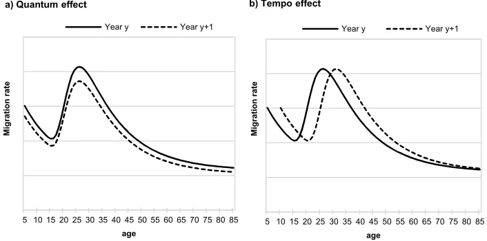
As in the case of fertility (Kohler and Ortega 2002), a secular shift in the age at migration may reflect two intertwined processes that would exert quite different impacts on overall migration levels: (1) a tempo effect leading to a temporary underestimation of the quantum, or level, of migration in observed period data and (2) a migration ageing effect leading to a reduction in higher-order moves because the exposure to migration is shifted to older ages when the probability of moving is lower.
In other words, the immediate effect of a delay in the age at migration is a tempo effect observable in period data, e.g., a small downward shift in the period measure of migration levels. If the age profile of migration subsequently stabilises at a new slightly older age profile, then period measures will subsequently bounce back. If, on the other hand, the delay of migration leads to a reduction in the total number of moves because the likelihood to move is lower at older ages, then period measures would register a secular downward shift. While conceptually distinct, these two effects are likely to occur concurrently. It is therefore not possible to disentangle the two simply by observing period measures; the timing of moves needs to be examined more directly. In a context of declining migration levels in a number of countries in the Organisation for Economic Co-operation and Development (OECD), understanding how tempo and ageing effects operate on migration behaviour and affect recorded period estimates of migration is of fundamental importance. Yet these processes are generally not recognised and are rarely, if ever, taken into account in the empirical analysis of migration.
progression to higher-order moves. This indicates that when migration is delayed to older ages, this shift is not made up by moves later in life and that period measures are likely to record a secular downward trend. The paper concludes that the analysis of migration data by move order offers a new perspective on migration behaviour that can shed light on well-established demographic problems such as tempo effects while highlighting the paucity of adequate migration data and the need to change migration data collection practices.
2. Tempo versus quantum effects
Ryder (1956, 1964) is credited with introducing the notion of tempo effects into the demographic literature. He demonstrated that changes in the timing of childbearing of cohorts resulted in a discrepancy between period (total fertility rate) and cohort (completed fertility rate) measures of fertility. More recently, Bongaarts and Feeney (1998) introduced an approach to estimating tempo effects that requires only period age-specific fertility rates by birth order. Drawing on this method, subsequent studies demonstrated that tempo effects cause an underestimation of quantum fertility in observed period data (Kohler and Ortega 2002; Sobotka 2003). Bongaarts and Feeney (2008) then broadened the notion of tempo effects to life-course events in general, including marriage and death, followed by a large body of literature that has demonstrated and quantified tempo effects in period measures of nuptiality (Winkler-Dworak and Engelhardt 2004) and death (Goldstein 2008; Luy 2006; Luy and Wegner 2009). Bongaarts and Feeney (2008) defined a tempo effect as a temporary, artificial inflation or deflation of the period measure of a demographic event because of a rise or fall in the mean age at which the event occurs. While the authors did not directly consider migration, their reasoning can apply equally to population movement.
American countries since the 1960s (Mulder 2009). In OECD countries, the average mean age at first birth now stands at 30 and above as a result of a two-to-five-year delay over the last two decades (Frejka and Sardon 2006; OECD 2018). If the delay in the age at migration simply shifts the age profile of migration to later ages, whereby delayed moves are later made up, the effect would be an underestimation of migration in observed period data (tempo effect) and period measures will subsequently bounce back. If, on the other hand, this shift leads to moves being foregone (ageing effect), period data would accurately reflect a downward shift in aggregate migration levels, with period measures registering a secular downward shift that would not be made up.
Figure 1: Hypothetical illustration of quantum and tempo effects
3. Impact of tempo effect on migration indicators
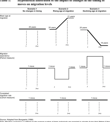
In this section, we seek to demonstrate the conditions under which changes in the timing of migration affect period measures of migration. Table 1 represents in a schematic form the impact of a rise and a fall in the mean age at migration on the migration expectancy (ME), which is defined as the average number of times individuals are expected to move during their lifetime if they conform to the age-specific migration and mortality rates of a given year (Bell et al. 2002; Long 1973). Table 1 compares the ME with the corresponding cohort indicator, the completed migration rate (CMR), which is the average number of moves among individuals of a given birth cohort (Bernard 2017b; Kolk 2016). Adapting Bongaarts’s (1999) example to migration, we assume a simple, hypothetical situation where every individual in each cohort moves once and all individuals move at the same age within each cohort. In scenario 1, individuals move at age 20 and there is no change between cohorts in the age at migration. Thus, period and cohort indicators are equal and remain stable at unity. In scenario 2, the age at migration is delayed from age 20 at timet to age 21 at time t+n. In this circumstance, the migration expectancy temporarily falls to 0.90 (negative tempo effect) before bouncing back to one, whereas the CMR remains stable at 1. Conversely, in scenario 3, the mean age at migration declines by one year to age
5 10 15 20 25 30 35 40 45 50 55 60 65 70 75 80 85
Migration rate
age a) Quantum effect
Year y Year y+1
5 10 15 20 25 30 35 40 45 50 55 60 65 70 75 80 85
Migration rate
age b) Tempo effect
19 at time t+n, leading to a temporary rise in migration expectancy to 1.1 moves (positive tempo effect) before returning to 1.
Table 1: Hypothetical illustration of the impact of changes in the timing of moves on migration levels
Scenario 1
No changes in timing Rising age at migrationScenario 2 Declining age at migrationScenario 3
Mean age at migration
Migration expectancy (Period measure)
Completed migration rate (Cohort measure)
Source: Adapted from Bongaarts (1999).
Note: Migration expectancy is defined as the average number of times individuals are expected to migrate during their lifetime if they conform to the age-specific migration and mortality rates of a given year. The completed migration rate is the average number of moves undertaken by members of a given cohort over the course of their lives.
Table 2 provides an illustration of tempo distortions caused by a continuous delay by showing hypothetical age-specific migration rates based on one-year migration data over a 35-year period reported over 5-year intervals. All periods display a typical age profile in which migration peaks at young adult ages and declines thereafter. However,
20 years
1 move
1 move 1 move 1 move
t t+n
t t+n
t t+n t t+n t t+n
20 years
21 years
t t+n
20 years
19 years
t t+n
t t+n
1 move 1 move 1 move 1 move
over successive periods there is a progressive delay of the modal age at migration from 20–24 years to 35–39 years and the migration intensity at peak progressively diminishes. The sum of mortality-adjusted age-specific migration rates down the columns, multiplied by five, gives the migration expectancy. By summing migration rates diagonally and multiplying them by five, one obtains the completed migration rate. Cohort data provides, however, a smaller number of observations, three versus eight for cross-section data. As Bongaarts and Feeney (2010) note, period and cohort measures are not necessarily equal even if they remain stable over a sustained period. Period and cohort indicators can be constant for a long period while not being equal if the mean age at migration is changing. In this particular example, over the 35-year period, the ME declined from 13 to 11 moves, while the CMR remained constant at 14.75 moves. In this situation, depressed period migration measures are therefore partly due to a delay of migration to older ages, while the quantum of migration remained stable. In other words, as individuals delay migrating, the observed period migration level is lower than it would have been without a tempo change. As in the case of fertility, the size of a tempo effect depends on the rate of change (and not the absolute value) of the mean age at migration (Bongaarts and Sobotka 2012; Sobotka 2003). Thus, the first step in identifying and gauging tempo effects is the reliable measurement of changes in the timing of migration.
Table 2: Hypothetical illustration of tempo effect: hypothetical
mortality-adjusted age-specific single-year migration rates by age group, period, and cohort migration indicators
Observation year
y y+5 y+10 y+15 y+20 y+25 y+30 y+35
Age g
ro
up
15–19 0.50 0.45 0.35 0.30 0.30 0.25 0.20 0.15
20–24 0.85 0.80 0.70 0.50 0.45 0.40 0.35 0.25
25–29 0.55 0.60 0.60 0.65 0.50 0.45 0.40 0.40
30–34 0.35 0.35 0.40 0.45 0.60 0.65 0.55 0.45
35–39 0.25 0.25 0.30 0.35 0.40 0.40 0.65 0.65
40–45 0.10 0.10 0.10 0.20 0.15 0.20 0.15 0.30
Period migration expectancy 13.00 12.75 12.25 12.25 12.00 11.75 11.50 11.00
Cohort completed migration rate 14.75 14.75 14.75
4. Measuring changes in the timing of migration
Having defined tempo effects, outlined conditions under which they may occur, and illustrated how they manifest on period measures of migration, this section aims to empirically investigate how the timing of migration has changed over the last few decades in a number of advanced economies. The most common summary measure of the age profile is the modal age at migration, or the age at which migration peaks (Bell et al. 2002; Bernard, Bell, and Charles-Edwards 2014; Rogers and Castro 1981). In the absence of population registers in many countries, population censuses remain the main source of migration data, measuring the proportion of individuals who changed residence in the previous one or five years (Bell et al. 2015b). While some countries measure migration over one-year intervals, migration is more commonly measured over five-year intervals (Bell et al. 2015b). Since age at migration is reported at the end of the interval, and assuming that moves are equally distributed over the five-year interval, moves took place on average at an age 2.5 years younger than the age that is reported. It is important to note that such data is for all moves, irrespective of their order.
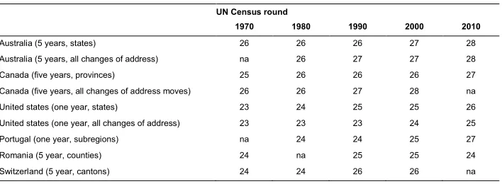
Table 3 reports the modal age at migration for all moves in six OECD countries, which have consistently collected migration data by single years of age for at least four decades and have made it publicly available (IPUMS 2017). While the age profile of migration is largely scale independent (Muhidin and Bell 2009), it is the best practice to analyse trends by using migration data collected over temporally consistent spatial units. We therefore report long-distance migration by using data for movements between major administrative units (i.e., states in the United States and Australia), which are typically subject to little or no changes in boundaries. Whenever possible we also report all changes of address in order to capture local moves, and we disaggregate migration intensities by single years of age. To avoid imposing an expected age distribution on the observed data, we used kernel regression, a non-parametric method (Bernard and Bell 2015), to smooth observed age-specific migration intensities rather than parametric approaches, such as exponential model migration schedules (Rogers and Castro 1981).
unity so that changes in the timing of migration can be identified independently from changes in its level. Results show that the ageing of the migration peak has been accompanied by a decrease in migration intensities, particularly at young adult ages. This decrease is especially pronounced in the United States, where the migration intensity at the peak has dropped by 45% over four decades from 55% in 1976 to 33% in 2016. Standardised migration intensities in Figure 2b clearly show that in both countries, the group of young adults moving in their twenties has fallen proportionally more than in other age groups. In Australia, the decrease has been less severe and there seems to have been a process of recuperation by which the ageing of the migration peak has been partially compensated by a rise in migration intensities in the thirties. In the United States, there is no evidence that this decline in mobility among young adults has been being made up at later ages: Thus the progressive decline in migration intensities at all ages is indicative of a quantum effect rather than a tempo effect.
Table 3: Modal age at migration, selected countries
UN Census round
1970 1980 1990 2000 2010
Australia (5 years, states) 26 26 26 27 28
Australia (5 years, all changes of address) na 26 27 27 28
Canada (five years, provinces) 25 26 26 26 27
Canada (five years, all changes of address moves) 26 26 27 28 na
United states (one year, states) 23 24 25 25 26
United states (one year, all changes of address) 23 23 23 24 25
Portugal (one year, subregions) na 24 24 25 27
Romania (5 year, counties) 24 na 25 25 24
Switzerland (5 year, cantons) 24 24 26 26 na
Figure 2: Age-specific migration intensities by year, Australia and the United States
Note: Migration data by single years of age, data smoothed using kernel regressions. In Figure 2b, migration intensities have been normalised to unity.
Source: As per Table 2. 0 10 20 30 40 50 60
1 5 9 13 17 21 25 29 33 37 41 45 49 53 57 61 65
Migration intensities Age 1986 1996 2006 2016 0 10 20 30 40 50 60
1 5 9 13 17 21 25 29 33 37 41 45 49 53 57 61 65
Migration intensities
Age
1976 1986 1996
2006 2016 0 1 2 3 4
1 5 9 13 17 21 25 29 33 37 41 45 49 53 57 61 65
Normalised migration intensities
Age 1986 1996 2006 2016 0 1 2 3 4
1 5 9 13 17 21 25 29 33 37 41 45 49 53 57 61 65
Nornalised m
igrati
on intensities
Age
1976 1986 1996
2006 2016
a) Australia, one year, all changes of address
b) Australia, one year, all changes of address
a) United States, one year, all changes of address
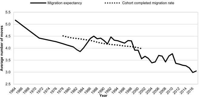
A long-time series of cohort and period measures can permit the detection of tempo effects (Bongaarts 1999), so we further investigate trends in migration in the United States by comparing period and cohort measures of migration. We use period life tables from the Human Mortality Database (Human Mortality Database 2018) to calculate survival ratios for each year and each age and draw migration data from the Current Population Survey, which represents the longest annual collection of internal migration data in the United States.3 Figure 3 reports the migration expectancy (ME) and the completed migration rate (CMR) estimated for ages 15 to 45, which are the ages at which most moves occur. Using intra-county moves by way of example, Figure 3 shows that both measures have decreased over the study period, although the cohort measure shows less variation than the period measure. The regularity of cohort time series compared with the often substantial fluctuations in period series is a well-established pattern in fertility studies (Ní Bhrolcháin 1992). With regard to migration, this can be readily explained by the fact that over the course of their lives, individuals pass through periods of high and low migration that are linked to cycles in the economy and housing markets (Cameron and Muellbauer 1998). Figure 3 shows a rebound in the migration expectancy in the mid-1980s through to the early 2000s, but the overall trend is downward, with migration expectancy dropping from a maximum of 5.2 moves in 1964 down to 3.5 and below since 2011. While the completed migration rate fluctuates less than the migration expectancy, it also exhibits a downward trend from an average of 4.5 down to 4.0 over the period. The latter confirms the presence of a quantum effect: Individuals are moving at progressively lower intensities. We observe similar trends for moves between counties and between states (not shown). While a visual inspection is useful to detect possible tempo and quantum effects, it does not permit their quantification.
Figure 3: Migration expectancy versus cohort completed migration rate, intra-county moves, the United States
Source: The Current Population Survey (1964–2017) and the Human Mortality Database (2018), authors’ calculations. CPS did not collect migration data for the following years: 1965–1970, 1972–1975, 1977–1980, 1985, and 1995. The data was linearly interpolated for missing years, which contributes to smaller variations in the first 15 years.
Note: Migration between the ages of 15 and 45 years. Migration expectancy is defined as the average number of times individuals are expected to migrate during their lifetime if they conform to the age-specific migration and mortality rates of a given year. The completed migration rate is the average number of moves undertaken by members of a given cohort over the course of their lives.
5. Order-specific changes in the timing of migration
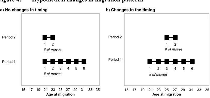
In this section, we argue that all-move data, such as those used in Section 4, is not suitable for the analysis of tempo effects because it conceals the extent of change in the timing of moves. We demonstrate this proposition with a simple hypothetical illustration from Bongaarts (1999) adapted to migration. We then validate it empirically by comparing trends in mean ages by move order in England and China. Figure 4 represents highly stylised patterns of migration at two points in time. In period 1, all individuals move six times, all at the exact same age, first time at age 21 and then every two years until age 31. The mean age at migration for all moves in that case is 26 years. In the second period, the average number of moves declines to two. In Figure 4a, the timing of the first and second moves remains constant at 21 and 23 years, respectively, but all individuals cease to migrate after two moves. In that case, the mean age at migration for all moves is 22 years. Using this indicator, one would assume that the timing of moves has been brought forward significantly, which is indicative of a large tempo effect. This is, however, an erroneous conclusion. The mean ages at first and second moves have not changed between the two periods. It is the disappearance of
2.5 3.0 3.5 4.0 4.5 5.0 5.5
A
verage
nu
mber
of
mov
es
Year
higher-order moves in period 2 that has led to an inaccurate assessment of changes in the timing of migration and ultimately to the incorrect identification of a tempo change. In Figure 4b, the onset of adult migration is delayed in period 2 by four years, with the mean age at first move progressing from 21 to 25. The mean age at migration for all moves is, however, the same for both periods, remaining stable at 26 years. This finding would lead to the incorrect conclusion that the age at migration has been stable in the absence of any tempo effects. In reality, the first and second moves have been substantially delayed, but when considering mean age at all moves, this effect is offset by the elimination of higher-order moves. Both scenarios illustrate how relying on all-move data can lead to erroneous conclusions about the evolution of the timing of migration, which in turn can result in the inaccurate identification of tempo effects.
Figure 4: Hypothetical changes in migration patterns
Source: Adapted from Bongaarts (1999).
These effects are clearly evident when we examine changes in the timing of migration by move order for cohorts born between 1918 and 1957 in England and between 1935 and 1969 in China. The first data set is drawn from the English Longitudinal Study of Ageing (ELSA), a longitudinal survey of the English population aged 50 and over (Marmot et al. 2016). Conducted in 2007, wave 3 retrospectively collected the complete residential mobility histories of individuals born between 1918 and 1957.4 These cohorts experienced important changes in migration behaviour among females but stable patterns for males. Among adult females, migration was
1 2 3 4 5 6
1 2
15 20 25 30 35
15 17 19 21 23 25 27 29 31 33 35 Age at migration
a) No changes in timing
Period 1 Period 2
# of moves # of moves
1 2 3 4 5 6
1 2
15 20 25 30 35
15 17 19 21 23 25 27 29 31 33 35 Age at migration
b) Changes in the timing
# of moves
# of moves
Period 2
progressively brought forward to earlier ages and the average number of moves increased (Falkingham et al. 2016), underpinned by a rise in the incidence of higher-order moves (Bernard 2017b). This period is therefore characterised by patterns of change opposite to current trends in most advanced economies where migration levels are trending down and mean ages at migration are rising.
Table 3 reports female mean ages at migration for all moves and by move order in England. Order-specific mean ages show that migration was brought forward by about three years for moves of all orders, whereas the mean age at migration for all moves was brought forward by only 1.8 years between the first and the last cohort. In that case, relying on all-move data would understate the extent of change in the timing of migration. As shown previously in Figure 4, this is likely to be caused by the inclusion of higher-order moves when considering mean ages for all moves. To understand order-specific changes in migration behaviour, Figure 5 displays for each cohort the proportion of females who moved at leasti times for moves up to the 10th move. Figure 5 reveals changes in the relative weights of moves of different orders. It shows that the proportion of females who moved at least three times increased from 30% for cohort 1 to 73% for cohort 4 and the proportion of those who moved at least seven times increased from 11% to 23%. Thus, females from cohort 4 started moving on average 2.6 years earlier than members of cohort 1 and a larger proportion moved multiple times and thus remained mobile later in life compared to cohort 1 members. Therefore, younger mean ages for lower-order moves are in part offset by the increase in higher-order moves, which take place at older ages, thereby moderating the apparent fall in the mean age at migration. This example shows that because changes in migration behaviour are order specific, all-move data can obscure the complexity of underlying changes and thus conceal the extent of changes in the timing of migration, which in turn may lead to misleading conclusions about tempo effects.
Table 3: Female mean age at migration by move order and for all moves by
birth cohort, England
Cohort 1
(1918–1927) Cohort 2(1928–1937) Cohort 3(1938–1947) Cohort 4(1948–1957) Difference between cohort 1and 4 (years)
Move 1 22.9 22.0 20.8 20.3 –2.6
Move 2 27.3 26.3 24.5 24.0 –3.3
Move 3 30.2 29.7 27.9 27.1 –3.1
Move 4 32.6 32.0 30.7 29.9 –2.7
Move 5 34.8 34.7 33.2 31.8 –3.0
All moves 29.4 29.3 28.1 27.6 –1.8
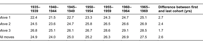
The analysis for England relates to a period where migration advanced to younger ages, but the same mechanisms apply to a delay in the age at migration. Table 4 reports male mean age at migration by move order and for all moves for cohorts born between 1935 and 1969 in China. The data was obtained from the Chinese Health and Retirement Longitudinal Study (CHARLS), which in 2014 retrospectively collected the lifetime migration histories of about 20,000 individuals over the age of 40. Order-specific mean ages show that migration has been pushed back to older ages. The first move was delayed by 2.7 years between the first and the last cohort, compared with 2.4 years for the second move and 1.7 years for the third move. Thus, the extent of changes in the timing of migration is order specific. These variations are hidden when considering the mean age at all moves, which indicates a 2.6 year delay. This is because repeated movement is rare in China and most migrants move only once or twice (Bernard, Bell, and Zhu 2019), thus the mean age at all moves is skewed in favour of the first and second moves. In this particular instance, the mean age at all moves is broadly similar to the mean age at the first move; nevertheless it conceals the extent of change in the timing of migration by obscuring the more modest shift in the age at moves of third order and higher.
Figure 5: Migration progression ratio by birth cohort, females
Source: ELSA, authors’ calculations, moves between the ages of 17 and 50.
Similar problems are likely to affect census data, such as those reported in Table 2, which accounts for moves of all orders and remains the main source of migration data in countries around the world (Bell et al. 2015b). As in the case of fertility, the solution
0.00 0.10 0.20 0.30 0.40 0.50 0.60 0.70 0.80 0.90 1.00
1 2 3 4 5 6 7 8 9 10
MI
gratio
n p
rogressio
n
ratio (0, i)
Move order
Cohort 1 Cohort 2
results also suggest that tempo effects should also be analysed separately for each move order because the rate of change in mean ages can differ by move order. While the solution is relatively straightforward conceptually, its practical application is more challenging because, as noted earlier, migration data is rarely collected by move order. However, population registers and administrative records permit the analysis of migration by move order from both a cohort and period perspective (Bernard and Kolk 2019; Kulu, Lundholm, and Malmberg 2018) and should therefore allow identifying tempo effects and assessing whether some delayed moves are made up later in life or are simply missed.
Table 4: Male mean age at migration by move order and for all moves by
birth cohort, China
1935–
1939 1940–1944 1945–1949 1950–1954 1955–1959 1960–1964 1965–1969 Difference between firstand last cohort (yrs)
Move 1 22.4 21.5 22.7 23.3 24.3 24.7 25.1 2.7
Move 2 24.5 23.6 24.7 25.8 26.5 26.6 26.9 2.4
Move 3 26.8 25.1 26.1 26.7 28.6 29.1 28.5 1.7
All moves 24.9 24.0 25.0 25.2 26.3 26.9 27.5 2.6
Source: China Health and Retirement Longitudinal Study (CHARLS), authors’ calculations, amended from Bernard, Bell, and Zhu (2019), moves between the ages of 17 and 40.
6. Migration ageing effect
We argued in the introduction that there is another mechanism, the ‘migration ageing effect,’ by which a delay in the age at migration may affect overall migration levels. A delay in the age at first move is likely to reduce higher-order moves because the exposure to migration is shifted to older ages when the probability of moving is lower. Conversely, if the age at migration is brought forward, the exposure to migration will be shifted to younger ages when the probability of moving is higher, which will increase the opportunities for progression to higher-order moves and, in turn, potentially lead to a higher overall migration level. Changes in the timing of migration therefore raise two key questions: (1) What is the impact of delayed age at first migration on completed lifetime migration, and (2) how much recuperation of migration is likely to occur at older ages?
decisions?” (Taeuber 1966: 418). The hypothesis of a link between the onset of migration and the overall level of migration was first supported by cross-sectional evidence from 10 European countries, which shows a strong negative correlation between mean ages at leaving the parental home and overall migration intensities (Bell et al. 2015a). Taking a cohort approach, Bernard (2017a) confirms a link between the onset of migration and completed migration rate at a macro level by showing a negative association between mean age at first move and cohort completed migration rates in 14 European countries. At an individual level, Bernard (2017b) shows for England that the age at first move operates to affect completed migration by influencing progressions to moves of higher order: the younger the age at first migration, the higher the likelihood of moving a second time, and vice versa. This proposition was further tested and confirmed in 14 European countries (Bernard 2017a) and in Australia and the United States (Bernard et al. 2017). These results suggest the presence of a migration ageing effect in the way that a delay in first adult migration tends to reduce lifetime migration at a cohort level. From a period perspective, this means that if young adults delay leaving the parental home, it will have an impact on their migration as they progress through life, which is likely to result in a further decline in the aggregate level of migration. What is now needed is to measure the extent of the hypothesised migration ageing effect by examining the impact of age at first adult move on completed migration in a larger sample of countries.
the two measures, with a Pearson correlation coefficient of 0.81, indicating that the age at leaving home is a good proxy for the start of the migration career of young adults.
Figure 5 plots mean age at leaving home against the completed migration rate for individuals born between 1961 and 1970 in each of the 26 countries. It shows a clear negative association, indicating that later ages at leaving the parental home are associated with reduced lifetime migration. The strength of this association is supported by a correlation coefficient of –0.77. Thus, Nordic countries combine high adult migration (more than five moves on average) and early mean age at leaving the parental home, before age 20 in Denmark, Sweden, and Finland. Conversely, countries in southern and eastern Europe exhibit the opposite patterns of low mobility with less than two moves on average and late departure from the parental home particularly in Portugal, Slovakia, Malta, and Italy.
Figure 5: Mean age at leaving home against the average number of moves after
departure
Source: Eurobarometer 64.1 collected in 2005. Results for individuals born between 1961 and 1970. Authors’ calculations. Sweden
Finland
Denmark
Northern Ireland France
Great Britain The Netherlands West Germany Ireland Belgium East Germany Luxembourg Spain Lithuania Latvia Hungary Austria Estonia Greece Slovenia Cyprus Poland Czech Republic Portugal Italy Slovakia Malta
y = -0.68x + 17.75 R² =0.59 0 1 2 3 4 5 6 7
19 20 21 22 23 24 25
A verage nu mber of mov es aft er hav ing left the pa ren tal h ome
Table 5: Odds ratios and confidence intervals of progression to the second move as a function of age at leaving home
odds ratios 95% Confidence interval odds ratios 95% Confidence interval
Cyprus 0.966 0.889 1.048 Germany West 0.811*** 0.738 0.891
Portugal 0.913** 0.859 0.971 Belgium 0.811*** 0.748 0.879
Slovakia 0.899*** 0.853 0.948 France 0.809*** 0.734 0.891
Italy 0.859*** 0.813 0.908 Latvia 0.801*** 0.743 0.863
Greece 0.857*** 0.813 0.903 Ireland 0.786*** 0.726 0.851
Hungary 0.851*** 0.803 0.902 Austria 0.781*** 0.73 0.836
Czech Republic 0.851*** 0.801 0.904 Estonia 0.781*** 0.721 0.846
Germany East 0.850** 0.763 0.946 Northern Ireland 0.768*** 0.656 0.898
Spain 0.842*** 0.795 0.893 Luxembourg 0.763*** 0.678 0.858
Malta 0.839*** 0.773 0.911 United Kingdom 0.748*** 0.682 0.82
Poland 0.834*** 0.784 0.889 Denmark 0.709*** 0.593 0.846
Lithuania 0.830*** 0.768 0.897 The Netherlands 0.676*** 0.61 0.749
Finland 0.830* 0.703 0.979 Sweden 0.671*** 0.566 0.796
Slovenia 0.815*** 0.762 0.871
Note: * p<0.05, ** p<0.01, *** p<0.001.
Source: Eurobarometer 64.1 collected in 2005. Results for individuals born between 1961 and 1970. Authors’ calculations. Note: countries ranked in decreasing order of odds ratios.
Figure 6: Age at leaving home against the progression ratio to the second
move, selected countries
Source: Data from Eurobarometer 64.1 collected in 2005. Results for individuals born between 1961 and 1970.
Note: Migration progression ratio to the second move is defined as the proportion of first-time movers who went on to move at least one more time.
0 0.1 0.2 0.3 0.4 0.5 0.6 0.7 0.8 0.9 1
18 19 20 21 22 23 24 25 26 27 28 29 30
Migration prog
ressio
n
ratio to the 2nd
mov
e
By influencing the progression to the second move, age at leaving home exerts an enduring effect on migration behaviour. As a result, late starters tend to exhibit lower levels of lifetime migration than those who left early. This can be seen in Figure 7, which displays age at leaving home against the completed migration rate for the Czech Republic and the Netherlands. In the latter, individuals who left home by age 20 reported on average 5 subsequent moves compared with 2.5 moves or less for individuals who left home at age 26 or later. Similarly, in the Czech Republic the completed migration rate decreases gradually with age at leaving home. The same patterns were observed in the other sample countries. These results demonstrate the presence of a migration ageing effect across Europe while revealing that the magnitude of this effect is context specific and varies from one country to the next. These findings highlight the importance of studying migration by move order and the need to pay particular attention to shifts in the timing of the first adult move to understand changes in migration levels. As late starters report lower progression to higher-order moves, they will display lower migration levels in the future as they progress through life. As a result, delays in the onset of adult migration will have an enduring effect on both period and cohort migration indicators.
Figure 7: Age at leaving home against completed migration rate, selected
countries
0 1 2 3 4 5 6 7
18 19 20 21 22 23 24 25 26 27 28
Com
pl
eted
m
igra
tion
rate
Age at leaving home
7. Discussion and conclusion
Understanding changes in migration is central to demographers and population geographers interested in measuring, understanding, and projecting migration. Despite recent advances in the field, migration scholars have not explicitly considered the impact of changes in the timing of migration on migration levels. Drawing on the fertility literature, we argue there are two intertwined processes by which changes in the timing of migration can affect overall migration levels: (1) a tempo effect, arising from a secular shift in the age at migration, which leads to an underestimation of the quantum, or level, of migration in the observed period data and (2) a migration ageing effect, which reduces higher-order moves because the exposure to migration is shifted to older ages when the probability of moving is lower. This paper proposes a framework for thinking about tempo and ageing effects of migration and assesses the types of data required to empirically analyse these processes.
We show that period indicators of migration, as in the case with other demographic processes, are likely to be distorted by tempo effects if the general trend is towards later ages at migration. In other words, the observed period migration level is likely to be lower than it would have been if the timing of migration had remained unchanged. The first step in the empirical analysis of tempo effects is the measurement of changes in the timing of migration. Analysis of census and survey data for Australia, Canada, the United States, Portugal, Romania, and Switzerland reveals that in all countries expect Romania, the modal age at migration has been delayed by two to three years since the 1970s, resulting in a shift in the peak age at migration from the mid-twenties to the late mid-twenties. Because the order of moves is typically not recorded in censuses and surveys, the modal age at migration accounts for moves of all orders (first, second, etc.). Using hypothetical scenarios, we show that all-move data is suitable for the measurement of tempo effects only if (1) the mean age at migration follows the same trend for moves of all orders and (2) the distribution of move order does not change over time. Using retrospective survey data from England and China, we empirically show that these two conditions are rarely met: Changes in migration behaviour are order specific. As a result, all-move data can obscure the complexity of underlying changes and thus conceal the extent of changes in the timing of migration, which in turn may lead to misleading conclusions about tempo effects.
been postponed to a greater extent than what all-move data suggests. However, because census and survey data rarely collect information on move order, the current understanding of the evolution of migration age patterns remains limited.
This paper argues that there is another linked mechanism by which changes in the ages at migration affect overall migration levels. The ‘migration ageing effect’ is thought to reduce higher-order moves because when the first migration is delayed, the exposure to migration is shifted to older ages when the probability of moving is lower. We test this proposition by examining adult migration by age at leaving the parental home in 26 European countries. After controlling for sex and birth cohort, we found that in all countries except Cyprus, younger movers were more likely to move at least once more after the first migration and, as a result, reported higher completed migration than late starters. Thus, further delays in the age at leaving the parental home would limit the number of migrations among young adults, with consequences not only in reducing current period indicators of migration directly but also potentially in future periods by decreasing their likelihood of moving later in life.
In this paper, we consider tempo and ageing effects separately as a first step in the conceptualisation of these processes for migration. What is now needed is a joint analysis to disentangle and quantify the relative importance of tempo and ageing effects in driving down period measures of migration levels. Methods developed in fertility research should permit such endeavours (see Kohler and Ortega 2002), although access to adequate data remains a challenge. The increasing collection of complete retrospective residential histories in Asia (China Health and Retirement Longitudinal Study in 2015), Europe (Survey of Health, Ageing and Retirement in Europe in 2007), North America (Health and Retirement Study in 2015), and Australia (Life Histories and Health Survey 2012) have been instrumental in providing new insights into order-specific changes in migration from a cohort perspective (Bernard 2017b, 2017a; Bernard et al. 2017; Falkingham et al. 2016; Vidal and Lutz 2018). However, retrospective migration surveys need to be repeated multiple times to permit a trend analysis of migration by move order, which is not yet a common practice. Alternatively, population registers and administrative records can be used to examine order-specific components of migration change from a period perspective and there are recent examples of such data sets used to identify period trends in order-specific migration rates (Kulu, Lundholm, and Malmberg 2018). However, while population registers are an important source of demographic data in Europe (Poulain and Herm 2013), publicly available aggregate migration indicators are not disaggregated by move order, and access to individual-level data follows strict access protocols that limits its use.
aggregate migration indicators by move order in the same way that they release parity-specific measures of fertility. In countries where such data is not available, repeated retrospective surveys offer the most cost-effective approach to obtain trends in period and cohort indicators of migration, although further research into recall error and survivor bias may be needed.
Access to such data in multiple countries would permit further testing of our proposition that changes in migration behaviour are order specific. This in turn would allow migration scholars to draw on important advances in the fertility literature over the last two decades to enhance understanding of migration trends. Bongaarts and Feeney’s (1998) method of correcting tempo effects suggests that period age-specific migration intensities by move order are sufficient to estimate tempo effects and generate tempo-adjusted period measures of migration. Application to migration would represent an important step forward in the analysis and understanding of migration as tempo effects can lead to a distorted view of trends, which in turn can lead to misleading projections and the adoption of suboptimal policies (Bongaarts and Feeney 2008).
8. Acknowledgements
References
Bell, M., Blake, M., Boyle, P., Duke-Williams, O., Rees, P., Stillwell, J., and Hugo, G. (2002). Cross-national comparison of internal migration: Issues and measures. Journal of the Royal Statistical Society Series A: Statistics in Society 165(3): 435–464.doi:10.1111/1467-985X.t01-1-00247.
Bell, M., Charles-Edwards, E., Bernard, A., and Ueffing, P. (2018a). Global trends in internal migration. In: Champion, T., Cooke, T.J., and Shuttleworth, I. (eds.). Internal migration in the developed world: Are we becoming less mobile? London: Routledge: 76–97.doi:10.4324/9781315589282-4.
Bell, M., Charles-Edwards, E., Kupiszewska, D., Kupiszewski, M., Stillwell, J., and Zhu, Y. (2015b). Internal migration data around the world: Assessing contemporary practice.Population, Space and Place 21(1): 1–17. doi:10.1002/ psp.1848.
Bell, M., Charles-Edwards, E., Ueffing, P., Stillwell, J., Kupiszewski, M., and Kupiszewska, D. (2015a). Internal migration and development: Comparing migration intensities around the world. Population and Development Review 41(1): 33–58.doi:10.1111/j.1728-4457.2015.00025.x.
Bell, M., Wilson, T., Charles-Edwards, E., and Ueffing, P. (2018b). Australia: The long-run decline in internal migration intensities. In: Champion, T., Cooke, T.J., and Shuttleworth, I. (eds.). Internal migration in the developed world: Are we becoming less mobile? London: Routledge: 147–172. doi:10.4324/978131558 9282-7.
Bernard, A. (2017a). Levels and patterns of internal migration in Europe: A cohort perspective.Population Studies 71(3): 293–311.doi:10.1080/00324728.2017.13 60932.
Bernard, A. (2017b). Cohort measures of internal migration: Understanding long-term trends.Demography 54(6): 2201–2221.doi:10.1007/s13524-017-0626-7. Bernard, A. and Bell, M. (2015). Smoothing internal migration age profiles for
comparative research. Demographic Research 32(33): 915–948. doi:10.4054/ DemRes.2015.32.33.
Bernard, A., Bell, M., and Charles-Edwards, E. (2014). Improved measures for the cross-national comparison of age profiles of internal migration. Population Studies 68(2): 179–195.doi:10.1080/00324728.2014.890243.
Bernard, A., Bell, M., and Charles-Edwards, E. (2016). Internal migration age patterns and the transition to adulthood: Australia and Great Britain compared.Journal of Population Research 33(2): 123–146.doi:10.1007/s12546-016-9157-0.
Bernard, A., Bell, M., and Zhu, Y. (2019). Migration in China: A cohort approach to understanding past and future trends. Population, Space and Place: e2234. doi:10.1002/psp.2234.
Bernard, A., Forder, P., Kendig, H., and Byles, J. (2017). Residential mobility in Australia and the United States: A retrospective study. Australian Population Studies 1(1): 41–54.
Billari, F.C. and Liefbroer, A.C. (2010). Towards a new pattern of transition to adulthood? Advances in Life Course Research 15(2): 59–75.doi:10.1016/j.alcr. 2010.10.003.
Bongaarts, J. (1999). The fertility impact of changes in the timing of childbearing in the developing world.Population Studies 53(3): 277‒289.
Bongaarts, J. and Feeney, G. (1998). On the quantum and tempo of fertility.Population and Development Review 24(2): 271–291.doi:10.2307/2807974.
Bongaarts, J. and Feeney, G. (2008). The quantum and tempo of life-cycle events. In: Barbi, E., Vaupel, J.W., and Bongaarts, J. (eds.). How long do we live? Demographic models and reflections on tempo effects. Berlin: Springer: 29–65. doi:10.1007/978-3-540-78520-0_3.
Bongaarts, J. and Feeney, G. (2010). When is a tempo effect a tempo distortion?Genus 66(2): 1–15.doi:10.4402/genus-188.
Bongaarts, J. and Sobotka, T. (2012). A demographic explanation for the recent rise in European fertility. Population and Development Review 38(1): 83–120. doi:10.1111/j.1728-4457.2012.00473.x.
Cameron, G. and Muellbauer, J. (1998). The housing market and regional commuting and migration choices. Scottish Journal of Political Economy 45(4): 420–446. doi:10.1111/1467-9485.00106.
Cooke, T. (2018). United States: Cohort effects on the long-term decline in migration rates. In: Champion, T., Cooke, T.J., and Shuttleworth, I. (eds.). Internal migration in the developed world: Are we becoming less mobile? London: Routledge: 101–119.doi:10.4324/9781315589282-5.
DeWaard, J., Johnson, J., and Whitaker, S. (2018). Internal migration in the United States: A comparative assessment of the utility of the consumer credit panel. Cleveland: Federal Reserve Bank of Cleveland (Working Paper 18-04). doi:10.26509/frbc-wp-201804.
Easterlin, R.A. (1974). Does economic growth improve the human lot? Some empirical evidence. In: David, P.A. and Reder, M.W. (eds.). Nations and households in economic growth. Cambridge: Academic Press: 89–125. doi:10.1016/B978-0-12-205050-3.50008-7.
Falkingham, J., Sage, J., Stone, J., and Vlachantoni, A. (2016). Residential mobility across the life course: Continuity and change across three cohorts in Britain. Advances in Life Course Research 30: 111–123.doi:10.1016/j.alcr.2016.06.001. Foster, T.B. (2017). Decomposing American immobility: Compositional and rate
components of interstate, intrastate, and intracounty migration and mobility decline.Demographic Research 37(47): 1515–1548.doi:10.4054/DemRes.2017. 37.47.
Frejka, T. and Sardon, J.-P. (2006). First birth trends in developed countries: Persisting parenthood postponement.Demographic Research 15(6): 147–180.doi:10.4054/ DemRes.2006.15.6.
Frey, H. (2017, November 20). US migration still at historically low levels, census shows. Brookings, The Avenue: Rethinking Metropolitan America. https://www.brookings.edu/blog/the-avenue/2017/11/20/u-s-migration-still-at-historically-low-levels-census-shows.
Furstenberg, F.F. (2013). Transitions to adulthood: What we can learn from the West. The Annals of the American Academy of Political and Social Science 646(1): 28–41.doi:10.1177/0002716212465811.
Goldscheider, F.K. and Goldscheider, C. (1999).The changing transition to adulthood: Leaving and returning home. Thousand Oaks: Sage.
Human Mortality Database (2018). Human Mortality Database [electronic resource]. Berkeley and Rostock: University of California and Max Planck Institute for Demographic Research.www.mortality.org.
IPUMS (2017). Integrated Public Use Microdata Series, International: Versions 6.5 [dataset]. Minneapolis: University of Minnesota.doi:10.18128/D020.V6.5. Kohler, H.-P. and Ortega, J.A. (2002). Tempo-adjusted period parity progression
measures: Assessing the implications of delayed childbearing for cohort fertility in Sweden, the Netherlands and Spain. Demographic Research 6(7): 145–190. doi:10.4054/DemRes.2002.6.7.
Kolk, M. (2016). Period and cohort measures of migration. Stockholm: Stockholm University, Demography Unit (Stockholm Research Reports in Demography 2016:5).doi:10.13140/RG.2.1.5171.2885.
Kulu, H., Lundholm, E., and Malmberg, G. (2018). Is spatial mobility on the rise or in decline? An order-specific analysis of the migration of young adults in Sweden. Population Studies 72(3): 323–337.doi:10.1080/00324728.2018.1451554. Lomax, N. and Stillwell, J. (2018). United Kingdom: Temporal change in internal
migration in the United Kingdom. In: Champion, T., Cooke, T.J., and Shuttleworth, I. (eds.). Internal migration in the developed world: Are we becoming less mobile? London: Routledge: 120–146.doi:10.4324/9781315589 282-6.
Long, L.H. (1973). New estimates of migration expectancy in the United States. Journal of the American Statistical Association 68(341): 37–43.
Luy, M. (2006). Mortality tempo-adjustment: An empirical application. Demographic Research 15(21): 561–590.doi:10.4054/DemRes.2006.15.21.
Luy, M. and Wegner, C. (2009). Conventional versus tempo-adjusted life expectancy: Which is the more appropriate measure for period mortality?Genus 65(2): 1–28. Marmot, M., Oldfield, Z., Clemes, S., Blake, M., Phelps, A., Nazroo, J., Steptoe, A., Rogers, N., Banks, J., and Oskala, A. (2016). English Longitudinal Study of Ageing: Waves 0–7, 1998–2015 [data collection]. Colchester: UK Data Service. doi:10.5255/UKDA-SN-5050-13.
Molloy, R., Smith, C.L., and Wozniak, A.K. (2014). Declining migration within the US: The role of the labor market. Cambridge: National Bureau of Economic Research (NBER Working Paper 20065).doi:10.3386/w20065.
Muhidin, S. and Bell, M. (2009). Cross national comparisons of internal migration in Asia-Pacific region. Paper presented at the Annual Meeting of the Population Association of America (PAA), Detroit, USA, April 30–May 2, 2009.
Mulder, C.H. (1993).Migration dynamics: A life course approach. Amsterdam: Thesis. Mulder, C.H. (2009). Leaving the parental home in young adulthood. In: Furlong, A. (ed.).Handbook of youth and young adulthood: New perspectives and agendas. London: Routledge: 203–210.
Ní Bhrolcháin, M. (1992). Period paramount? A critique of the cohort approach to fertility.The Population and Development Review 18(4): 599–629.doi:10.2307/ 1973757.
OECD (2018). Age of mothers at childbirth and age-specific fertility. Paris: OECD, Social Policy Division, Directorate of Employment, Labour and Social Affairs. https://www.oecd.org/els/soc/SF_2_3_Age_mothers_childbirth.pdf.
Pandit, K. (1997a). Cohort and period effects in US migration: How demographic and economic cycles influence the migration schedule.Annals of the Association of American Geographers 87(3): 439–450.doi:10.1111/1467-8306.00062.
Pandit, K. (1997b). Demographic cycle effects on migration timing and the delayed mobility phenomenon. Geographical Analysis 29(3): 187–199. doi:10.1111/ j.1538-4632.1997.tb00956.x.
Pelikh, A. and Kulu, H. (2018). Short-and long-distance moves of young adults during the transition to adulthood in Britain.Population, Space and Place 24(5): e2125. doi:10.1002/psp.2125.
Plane, D.A. and Rogerson, P.A. (1991). Tracking the baby boom, the baby bust, and the echo generations: How age composition regulated US migration. The Professional Geographer 43(4): 416–430. doi:10.1111/j.0033-0124.1991.0041 6.x.
Rogers, A. and Castro, L.J. (1981). Model migration schedules. Laxenburg: International Institute for Applied Systems Analysis (Research Report RR-81-30).
Rogers, A. and Rajbhandary, S. (1997). Period and cohort age patterns of US migration, 1948–1993: Are American males migrating less? Population Research and Policy Review 16(6): 513–530.doi:10.1023/A:1005824219973.
Rogerson, P.A. (1987). Changes in US national mobility levels. The Professional Geographer 39(3): 344–351.doi:10.1111/j.0033-0124.1987.00344.x.
Ryder, N.B. (1956). Problems of trend determination during a transition in fertility.The Milbank Memorial Fund Quarterly 34(1): 5–21.doi:10.2307/3348329.
Ryder, N.B. (1964). The process of demographic translation.Demography 1(1): 74–82. doi:10.2307/2060032.
Saks, R.E. and Wozniak, A. (2007). Labor reallocation over the business cycle: New evidence from internal migration. Bonn: IZA (IZA Discussion Paper No. 2766). Shuttleworth, I., Osth, J., and Niedomysl, T. (2018). Sweden: Internal migration in a
high-migration Nordic country. In: Champion, T., Cooke, T.J., and Shuttleworth, I. (eds.). Internal migration in the developed world: Are we becoming less mobile? London: Routledge: 203–225.doi:10.4324/9781315589282-9.
Sobotka, T. (2003). Tempo-quantum and period-cohort interplay in fertility changes in Europe: Evidence from the Czech Republic, Italy, the Netherlands and Sweden. Demographic Research 8(6): 151–214.doi:10.4054/DemRes.2003.8.6.
Stone, J., Berrington, A., and Falkingham, J. (2014). Gender, turning points, and boomerangs: Returning home in young adulthood in Great Britain.Demography 51(1): 257–276.doi:10.1007/s13524-013-0247-8.
Taeuber, K.E. (1966). Cohort migration. Demography 3(2): 416–422. doi:10.2307/ 2060167.
Vidal, S. and Lutz, K. (2018). Internal migration over young adult life courses: Continuities and changes across cohorts in West Germany. Advances in Life Course Research 36: 45–56.doi:10.1016/j.alcr.2018.03.003.