Vol. 4, No. 3, Year 2012 Article ID IJIM-00245, 9 pages Research Article
Numerical Solution of Volterra-Fredholm Integral
Equations with The Help of Inverse and Direct
Discrete Fuzzy Transforms and Collocation
Technique
Reza Ezzatia∗, Fatemeh Mokhtaria, Mohammad Maghasedia
(a)Dapartment of Mathematics, Karaj Branch, Islamic Azad University, Karaj, Iran.
——————————————————————————————————
Abstract
In this paper, a new approach to the numerical solution of Volterra- Fredholm integral equations by using expansion method based on the composition of the inverse and direct discrete fuzzy transforms (shortly F-transforms) in combination with the collocation tech-nique is proposed. First, the unknown function is approximated by using the composition of the inverse and direct discrete F-transforms based on the fuzzy partition, then the Volterra- Fredholm integral equation is reduced to the linear system of equations. More-over, the convergence theorem for the proposed method is given in terms of the modulus of continuity. Finally, illustrative examples are included to show the accuracy and the efficiency of the proposed method.
Keywords: Volterra-Fredholm integral equation; Basic function; Fuzzy transforms.
—————————————————————————————————–
1
Introduction
For solving Volterra-Fredholm integral equations, many methods with enough accuracy and efficiency have been used before by many researches [6, 7, 8, 9, 10, 11, 12, 13, 14, 15]. Maleknejad and Fadaei Yami [11] solved the system of Volterra-Fredholm integral equa-tions by Adomian decomposition method. Maleknejad and Hadizadeh [12] proposed a new computational method for this kind of equation. Kauthen in [10], used continuous time collocation method for Volterra-Fredholm integral equations. In [24], Yalsinbas devel-oped numerical solution of nonlinear Volterra-Fredholm integral equations by using Taylor polynomials. Legendre wavelets also were applied for solving Volterra-Fredholm integral equations [25]. Maleknejad and Mahmodi in [13] applied Taylor polynomials for solving
∗Corresponding author. Email address: [email protected]
high-order Volterra-Fredholm integro-differential equations.
In classic mathematics, various kinds of transforms are used as powerful tools in the con-struction of approximation methods and especially for computing the numerical solution of integral equations. F-transform was proposed by Perfilieva and Chaldeeva [18] and studied in several papers [16, 17, 18, 20, 21, 22, 23]. Stepnikca and Valasek [23] have ap-plied F-transforms to solve partial differential equations numerically. Recently, Ezzati and Mokhtari proposed a new approach to numerical solution of Fredholm integral equations of the second kind by using F-transform. Solving differential equations through the data analysis by the fuzzy approach is done by Martino, Loia and Seaaa [4]. They constructed a basic function corresponding to the given function in order to approximate it in the first step. Approximation properties of the F-transforms were studied in [2, 16, 20]. The success of these applications is due to the fact that F-transforms are capable to accurately approximate any continuous function.
We decide to show, how this technique can be used to obtain numerical solution of Volterra-Fredholm integral equations. In the structure of Volterra-Volterra-Fredholm integral equation, we use inversion form of F-transform instead of precise representation of the original function. Then we form the linear system of equations. So, we can find its unknowns by this process. Here, we will apply the F-transform to approximate the unknown functions f(x), which we have let as the solution of Volterra-Fredholm integral equations as follows:
f(x) =g(x) +
∫ x
a
k1(x, t)f(t)dt + ∫ b
a
k2(x, t)f(t)dt , x∈[a, b]. (1.1)
Some basic definitions for F-transforms are presented subsequently. Section 3 investigates the mathematical formulation of proposed method. In Section 4, we present the error analysis of proposed method. In Section 5, some numerical results are provided. Finally, Section 6 gives our concluding remarks.
2
Preliminaries
Consider a Volterra-Fredholm integral equation of the second kind defined in Eq. (1.1), in which the function g(x) and kernelk(x, t) are given and the function f(x) is unknown. We take an interval [a, b] as a universe. The fuzzy partition of the universe is given by fuzzy subsets of the universe [ai, bi] determined by their membership function which must have the properties described in the following definition.
Definition 2.1. [16] Letx1< . . . < xnbe fixed nodes within[a, b]such thatx1=a, xn=b
and n≥2. We say that fuzzy sets A1, . . . , An, identified with their membership functions
A1(x), . . . , An(x)defined on[a, b], form a fuzzy partition of[a, b]if they fulfill the following
conditions for k= 1, . . . , n:
(a) Ak : [a, b]−→[0,1], Ak(xk) = 1;
(b) Ak(x) = 0 if x /∈(xk−1, xk+1) where for the uniformity of denotation, we put x0 = a, xn+1 =b;
(c) Ak(x) is continuous;
(d) Ak(x), k = 2, . . . , n, strictly increases on [xk−1, xk] and Ak(x), k = 1, . . . , n−1,
(e) for allx∈[a, b]
n
∑
k=1
Ak(x) = 1.
The membership functionsA1, . . . , An are called basic functions.
Definition 2.2(17). LetA1, . . . , Anbe basic functions which form a fuzzy partition of[a, b]
and f be any function fromC([a, b]). We say that the n-tuple of real numbers [F1, . . . , Fn]
given by
Fk=
∫b
a∫f(x)Ak(x)dx b
aAk(x)dx
is the (integral) F-transform of f with respect to A1, . . . , An. Let us remark that this
definition is correct because for eachk= 1, . . . , nthe productf Akis an integrable function
on [a, b].
Denote the F-transform of a function f with respect to A1, . . . , An by Fn[f]. Then, according to Definition 2.2, we can write
Fn[f] = [F1, . . . , Fn].
The elements F1, . . . , Fn are called components of the F-transform.
Lemma 2.1. Letf be a continuous function on[a, b]andA1, . . . , An,n≥3 be basic
func-tions which form a uniform fuzzy partition of [a, b], but function f be twice continuously differentiable in (a, b). Then for eachk= 1, . . . , n
Fk=f(xk) +O
( h2) .
Proof. For proof, see [16].
Definition 2.3. [16] LetA1, . . . , Anbe basic functions which form a fuzzy partition of[a, b]
and f be a function fromC([a, b]). LetFn[f] = [F1, . . . , Fn]be the integral F-transform of f with respect toA1, . . . , An. Then the function
fF,n(x) = n
∑
k=1
FkAk(x),
is called the inverse F-transform.
The following theorem shows that the inverse F-transform,fF,n, can approximate the original continuous functionf with an arbitrary precision.
Lemma 2.2. Let f be a continuous function on[a, b]. Then for anyε >0 there exists nε
and a fuzzy partitionA1, . . . , Anε of [a, b] such that for all x∈[a, b]
|f(x)−fF,nε(x)| ≤ε,
wherefF,nε(x)is the inverse F-transform offwith respect to the fuzzy partitionA1, . . . , Anε .
Definition 2.4. [16] Suppose that function f is given at nodes p1, . . . , pl ∈ [a, b] and
A1, . . . , An, n < l, be basic functions which form a fuzzy partition of [a, b]. We say that
the n-tuple of real numbers [F1, . . . , Fn] is the discrete F-transform of f with respect to
A1, . . . , An if
Fk=
∑l
j=1f(pj)Ak(pj)
∑l
j=1Ak(pj)
.
In the discrete case, we define the inverse F-transform only at nodes where the original function is given.
Through the paper, we suppose l=n.
Definition 2.5. [16] Let function f be given at nodes p1, . . . , pl ∈ [a, b] and Fn[f] = [F1, . . . , Fn]be the discrete F-transform of f w.r.t. A1, . . . , An. Then the function
fnF(pj) = n
∑
k=1
FkAk(pj),
defined at the same nodes, is the inverse discrete F-transform.
Definition 2.6. [1] Letf : [a, b]→R be a bounded function. Then
ω(f, δ) : [0,∞)→[0,∞)
defined by
ω(f, δ) = sup{ |f(x)−f(y)| : x, y ∈ [a, b], |x−y| ≤ δ}
is called the first order modulus of smoothness of f. If f is continuous then ω(f, δ) is called the uniform modulus of continuity.
Theorem 2.1. [1] The following properties hold true: (i) |f(x)−f(y)| ≤ ω(f, d(x, y)) for anyx, y ∈ [a, b]; (ii) ω(f, δ) is continuous in δ;
(iii) ω(f, δ) = 0;
(iv) ω (f, δ1+δ2)≤ ω (f, δ1) +ω (f, δ2) for any δ1, δ2 ∈ [0,∞);
(v) ω (f, n δ)≤ n ω (f, δ) for anyδ ∈ [0,∞) and n∈N; (vi) ω (f, λ δ)≤ (λ+ 1)ω (f, δ) for any δ, λ ∈ [0,∞); (vii) If f is continuous then limδ→0ω(f, δ) = 0.
Let n and k be arbitrarily fixed. The composition between the direct and inverse F-transform can be expressed as [2]
Fn, k(x) = k
∑
i=1 Ai(x)
∑n
j∑=1Ai(xj)f(xj)
n
j=1Ai(xj)
,
and f(x) can be rewritten as
f(x) = k
∑
i=1 Ai(x)
∑n
j∑=1Ai(xj)f(x)
n
j=1Ai(xj)
Theorem 2.2. Let y1, . . . , yk∈[a, b]be a partition of the interval [a, b] having the norm
δ. If A ={A1, . . . , Ak} is a fuzzy partition with small support, then the following error
estimate holds true:
|Fn,k(x)−f(x)| ≤rω(f, δ) , ∀x∈[a, b],
where Fn,k(x) denotes the composition of the inverse and direct discrete F- transform.
Proof. For proof, see [2].
3
Proposed method
In this section, we consider Eq. (1.1). For solving this kind of integral equations numeri-cally, the unknown function, f(x), is approximated byFn,n(x). By substituting Fn,n(x) instead of the unknown function, f(x),inside of integrals, we have:
f(x)∼=g(x) +
∫ x
a
k1(x, t)Fn,n(t)dt +
∫ b
a
k2(x, t)Fn,n(t)dt ,
where Ai(x), i= 1, . . . , n, are introduced in the previous section. Therefore, we have:
f(x)∼=g(x) +
∫ x
a
k1(x, t)
( n ∑
i=1 (∑n
k∑=1f(xk)Ai(xk) n
k=1Ai(xk) )
Ai(t)
) dt+
∫ b
a
k2(x, t) ( n
∑
i=1 (∑n
k∑=1f(xk)Ai(xk)
n
k=1Ai(xk)
) Ai(t)
) dt ,
f(x)∼=g(x) + n
∑
k=1 f(xk)
( n ∑
i=1
Ai(xk)
∑n
k=1Ai(xk)
∫ x
a
k1(x, t)Ai(t)dt )
+
n
∑
k=1 f(xk)
( n ∑
i=1
Ai(xk)
∑n
k=1Ai(xk)
∫ b
a
k2(x, t)Ai(t)dt
) .
If we set x=xj,j= 1, . . . , n, then we conclude the linear system of equations as follows:
f(xj)∼=g(xj) + n
∑
k=1 f(xk)
( n ∑
i=1
Ai(xk)
∑n
k=1Ai(xk)
∫ xj
a
k1(xj, t)Ai(t)dt )
+ n
∑
k=1 f(xk)
( n ∑
i=1
Ai(xk)
∑n
k=1Ai(xk)
∫ b
a
k2(xj, t)Ai(t)dt
) .
Equivalently, it can be solved the following linear system of equations:
BX=y, (3.2)
where B= (bij),i, j= 1, . . . , n,
bii= 1− n
∑
m=1
Am(xi)
∑n
k=1(Am(xk))
(∫ xi
a
k1(xi, t)Am(t)dt−
∫ b
a
k2(xi, t)Am(t)dt
bij =− n
∑
m=1
Am(xj)
∑n
k=1(Am(xk))
(∫ xi
a
k1(xi, t)Am(t)dt
∫ b
a
k2(xi, t)Am(t)dt
)
, i̸=j,
X= [f(x1) , f(x2), . . . , f(xn)]t, y= [g(x1), g(x2) , . . . , g(xn) ] t.
By solving the system BX = y, we can obtain f(xi),i = 1, . . . , n. Substituting f(xi), i= 1, . . . , n, in Fk defined in Definition 2.4, we can compute Fn,n(x) =
∑n
i=1FiAi(x) as an approximation off(x). For solving the systemBX =y, it is clear that matrixB must be invertible. So, we give the following theorem.
Theorem 3.1. Let B be an n×n matrix as introduced in Eq. (3.2), and let M1 =
supx,t∈[a,b]|k1(x, t)|,M2 = supx,t∈[a,b]|k2(x, t)|. If
M1+M2 <
1 (b−a),
then B is invertible.
Proof: We prove that ∥I−B∥∞<1. We have
∥I−B∥∞= max
1≤i≤n n
∑
j=1
|bij|
= max
1≤i≤n
∑n
j=1
n
∑
m=1
Am(xj)
∑n
k=1(Am(xk))
(∫ xi
a
k1(xi, t)Am(t)dt−
∫ b
a
k2(xi, t)Am(t)dt
)
≤ max
1≤i≤n
∑n
j=1
n
∑
m=1
|Am(xj)|
|∑n
k=1(Am(xk))|
(∫ xi
a
|k1(xi, t)|Am(t)dt+
∫ b
a
|k2(xi, t)|Am(t)dt
)
≤(b−a) (M1+M2)<1.
Now, by using Neuman series, we conclude that (I−(I−B))−1 = B−1 exists. This completes the proof.
4
Error analysis
Now, we present the convergence theorem, that justifies proposed method for approximat-ing solution of Eq. (1.1). Let (C([a, b]),∥ .∥) be the space of all continuous functions on interval [a, b] with the norm ∥f∥∞ = max
x∈[a,b]|f(x)|. We suppose that g(x) ̸= 0, and M1 = supx,t∈[a,b]|k1(x, t)|,M2 = supx,t∈[a,b]|k2(x, t)|. With these conditions, we have the
following theorem.
Theorem 4.1. Let y1, . . . , yn∈[a, b]be a partition of the interval[a, b]having the norm
in (a, b). Let Fn,n(x) be the approximate solution of Eq. (1.1). Then the absolute error
of approximate solution can be estimated as follows:
|f(x)−Fn,n(x)| ≤ r (M1+M2) (b−a) ω(f, δ).
Proof: Clearly, we have
|f(x)−Fn,n(x)|=
|
∫ x
a
k1(x, t)f(t)dt+ ∫ b
a
k2(x, t)f(t)dt− ∫ x
a
k1(x, t)Fn,n(t)dt−
∫ b
a
k2(x, t)Fn,n(t)dt|
=|
∫ x
a
k1(x, t) (f(t)−Fn,n(t))dt+
∫ b
a
k2(x, t) (f(t)−Fn,n(t))dt
≤
∫ x
a
k1(x, t) ( k
∑
i=1 Ai(t)
∑n
j=1Ai(xj)|f(t)−f(xj)|
∑n
j=1Ai(xj)
) dt+
∫ b
a
k2(x, t) ( k
∑
i=1 Ai(t)
∑n
j=1Ai(xj)|f(t)−f(xj)|
∑n
j=1Ai(xj)
) dt.
We observe that the product Ai(t)Ai(xj) = 0̸ if and only if t, xj ∈[yi, yi+r], and in this
case we have |t−xj| ≤rδ. By using Theorem 2.2, we conclude that:
f(x)−fnF(x)≤ ∫ax|k1(x, t)| r ω(f, δ) dt+ ∫b
a|k2(x, t)| r ω(f, δ) dt
≤ r(M1+M2) (b−a) ω(f, δ) .
5
Numerical examples
In order to show the accuracy of the proposed method, we present two examples. Software ”Mathematica7” is applied for computing results.
Example 5.1. [8] Consider the equation
f(x) =x−2ex+e−x+ 1 +
∫ x
0
yexf(y)dy+
∫ 1
0
e(x+y)f(y)dy.
The exact solution of this equation is as follows:
f(x) =e−x.
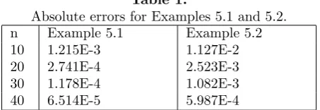
For comparing numerical and exact solutions, see Table1.
Example 5.2. [8] Consider the Volterra-Fredholm integral equation:
f(x) = cos (x)
(
1 2x−
1 4
)
+1
4cos (2−x) +
∫ x
0
sin (x−t)f(t)dt+
∫ 1
0
cos (x−t)f(t)dt,
The exact solution of this equation is as follows:
f(x) = sin (x).
Table 1.
Absolute errors for Examples 5.1 and 5.2.
n Example 5.1 Example 5.2
10 1.215E-3 1.127E-2
20 2.741E-4 2.523E-3
30 1.178E-4 1.082E-3
40 6.514E-5 5.987E-4
6
Conclusions
We used the composition of inverse and direct discrete F-transform to approximate the nu-merical solution of Volterra-Fredholm integral equations. The properties of basic functions and the F-transform provided us the possibility of reducing Volterra- Fredholm integral equation to a system of linear equations. The numerical and exact solutions are compared by considering the absolute error in two examples. The results show that the proposed approach can be a suitable method for solving Volterra-Fredholm integral equations nu-merically.
References
[1] GA. Anastassiou, SG. Gal, Approximation Theory: Moduli of Continuity and Global Smoothness Preservation, Birkhauser, Boston, Basel, Berlin, (2000).
[2] B. Bade, IJ. Rudas, Approximation properties of fuzzy transforms, Fuzzy Sets and Systems doi: 10.1016/j.fss.2011.03.001.
[3] M. Dankova, M. Stepnicka, Fuzzy transform as an additive normal form, Fuzzy Sets and Systems 157 (2006) 1024-1035.
[4] F. Di Martino, V. Loia, S. Sessa, Fuzzy transforms method and attribute dependency in data analysis, Information Sciences 180 (2010) 493-505.
[5] F. Di Martino, V. Loia, I. Perfilieva, S. Sessa, An image coding/decoding method based on direct and inverse fuzzy transforms, International Journal of Approximate Reasoning 48 (2008) 110-131.
[6] R. Ezzati, F. Mokhtari, Numerical solution of Fredholm integral equations of the second kind by using fuzzy transforms, International Journal of Physical Science, 7 (2012) 1578- 1583.
[7] R. Ezzati, S. Najafalizadeh,Numerical solution of nonlinear Voltra-Fredholm integral equation by using Chebyshev polynomials, Mathematical Sciences Quarterly Journal, 5 (2011) 14-22.
[8] R. Ezzati, S. Najafalizadeh, Numerical methods for solving linear and nonlinear Volterra-Fredholm integral equations by using CAS wavelets, To appear in World Ap-plied Sciences Journal.
[10] PG. Kauthen,Continuous time collocation methods for Voltra-Fredholm integral equa-tions, Numer Math 56 (1989) 409-424.
[11] K. Maleknejad, MR. Fadaei Yami, A computational method for system of Volterra-Fredholm integral equations, Appl. Math. Comput., 188 (2006) 589-595.
[12] K. Maleknejad, M. Hadizadeh, A new computational method for Volterra-Fredholm integral equation, J. Comput. Math. Appl. 37 (1999) 37-48.
[13] K. Maleknejad, Y. Mahmodi, Taylor polynomial solution of high-order nonlinear Volterra-Fredholm integro-differential equations, Appl. Math. Comput. 145 (2003) 641-653.
[14] K. Maleknejad, S. Sohrabi. Y. Rostami, Numerical solution of nonlinear Voltra inte-gral equation of the second kind by using Chebyshev polynomials, Appl. Math. Com-put. 188 (2007) 123-128.
[15] K. Maleknejad, M. Tavassoli, Y. Mahmoudi, Numerical solution of linear Fredholm and Volterra integral equations of the second kind by using Legendre wavelet, Kybern Int. J. Syst. Math. 32 (2003) 1530-1539.
[16] I. Perfilieva, Fuzzy transforms: theory and applications, Fuzzy Sets and Systems 157 (2006) 993-1023.
[17] I. Perfilieva,Fuzzy transforms: application to reef growth problem, in: R.B. Demicco, G.J. Klir (Eds.), Fuzzy Logic in Geology, Academic Press, Amesterdam, 13 (2003) 275-300.
[18] I. Perfilieva, Fuzzy transforms and their applications to data compression, In: Proc. Int. Conf. on FUZZ IEEE 2005, Reno, USA, May 22 (2005) 294-299.
[19] I. Perfilieva, E. Chaldeeva, Fuzzy transformation, in: Proc. Of IFSA’2001 World Congress, Vancouver, Canada, 2001.
[20] I. Perfilieva, Fuzzy transforms, in: J.F. Peters, et al. (Eds.), Transactions on Rough Sets II, Lecture Notes in Computer Science, 31 (2004) 63-81.
[21] I. Perfilieva, M. Dankova, Towards Fuzzy transforms of a higher degree, in: Proceed-ings of the IFSA-EUSFLAT Conference (2009) 585-588.
[22] D. Plskova, Fuzzy transform in geological applications, J. Electrical engineering, 105 (2006) 12-19.
[23] M. Stepnicka, R. Valasek, Numerical solution of partial differential equations with help of fuzzy transform, In: Proc. Int. Conf. on FUZZ IEEE 2005, NV. Reno, USA, June (2005) 1104-1109.
[24] S. Yalsinbas,Taylor polynomial solution of nonlinear Volterra-Fredholm integral equa-tions, Appl. Math. Comput. 127 (2002) 195-206.