Wiener
numbers
of
random
pentagonal
chains
HONGYONG WANG1,JIANG QIN1 AND IVAN GUTMAN2,
1School of Mathematics and Physics, University of South China, Hengyang 421001, Hunan,
P. R. China
2Faculty of Science, University of Kragujevac, P. O. Box 60, 34000 Kragujevac, Serbia
(Received April 7, 2013; Accepted April 25, 2013)
A
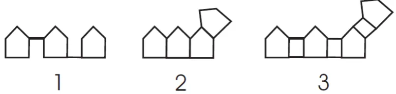
BSTRACTThe Wiener index is the sum of distances between all pairs of vertices in a connected graph. In this paper, explicit expressions for the expected value of the Wiener index of three types of random pentagonal chains (cf. Fig. 1) are obtained.
Keywords: Wiener index, pentagonal chain.
1.
I
NTRODUCTIONThe Wiener index is the oldest molecular structure descriptor, invented as early as in 1947 by Harold Wiener [18]. Initially it was ignored by the chemical community, and so it happened that Rouvray [16] independently re-invented it in 1975. The precise mathematical definition of the Wiener index (in terms of distance in graphs) was given in 1971 by Hosoya [9]. Mathematicians arrived at the very same idea somewhat later [5], but also independently.
Eventually, the Wiener index attracted the attention of chemists, due to its correlation with a large number of physico–chemical properties of organic molecules. It also attracted the attention of mathematicians due to its interesting and non-trivial mathematical properties.
Anyway, in the last 20-30 years an enormous amount of work was done on the study of the Wiener index. Ante Graovac also participated in these researches (see, for instance, [7, 11]). It is particularly worth noting that in the years that preceded his untimely death, the study of Wiener index and other distance–based structure descriptors, as well as
their applications to fullerenes and nanomolecules, was Ante Graovac’s main scientific interest [1–4, 6, 10, 12, 13, 17].
Let G be a connected graph with vertex set V = {v1, v2, … , vn}. The distance d(vr, vs)
between the vertices vrand vsin G is the number of edges of a shortest path between vrand
vs. The Wiener index is the sum of distances between all pairs vertices and is defined by
s r
n
r
n
r r
n
s r s
s
r v d v v d v G
v d G
W
1 1 1
) ( 2 1 ) , ( 2
1 ) , ( )
(
where d(vr|G) is the distance number of the vertex vr, defined by
. ) , ( )
(
1
n
s
s r
r G d v v
v d
Motivated by the works [8] and [19], in the present paper we establish explicit expressions for the expected value of the Wiener index of three types of random pentagonal chains, shown as Fig. 1.
Fig. 1. The three types of pentagonal chains (pentachains) examined in this paper: alpha
(1), beta (2), and gamma (3).
The following lemma is the main tool in the proof of our results.
Lemma 1. Let{tn}be a real number sequence satisfying
tn= q tn−1 + d n3 + a n2 + bn + c ; n ≥1 . (1)
If t0 = 0 and q1, then
tn= d I0 + a I1 + b I2 + c I3 (2)
where
] 4
) 1 3 3 (
) 4 6 3 ( ) 1 3 3 3 ( [ ) 1 (
1
3 2 1
3 2
3
2 2
3 2
3 3 4 0
n n
n q q
q q n n n
q n
] )
1 2 ( ) 1 2 2 ( [
) 1 (
1 2 2 2 2 1 2
3
1
n n n q n n q qn qn
q I
] )
1 ( [ ) 1 (
1 1
2
2
n n q qn
q I
. 1 1
3 q
q
I n
Proof.From (1), we have
tn= q tn−1 + d n3 + a n2 + bn + c
tn−1 = q tn−2 + d(n −1)3 + a(n −1)2 + b(n −1) + c tn−2 = q tn−3 + d(n −2)3 + a(n −2)2 + b(n −2) + c t2 = q t1 + d 23 + a 22 + 2b + c
t1 = q t0 + d 13 + a 12 + 1b + c .
The above formulas imply
tn= d n3 + d q(n −1)3 + d q2(n −2)3 + · · · + d qn−223 + d qn−113
+ a n2 + a q(n −1)2 + a q2(n −2)2 + · · · + a qn−222 + a qn−112 + b n + b q(n −1) + b q2(n −2) + · · · + b qn−22 + b qn−11
+ c + c q + c q2 + · · · + c qn−2 + c qn−1 = d I0 + a I1 + b I2 + c I3.
I3 is a geometric sequence with the common ratio q. Hence,
. 1 1
3 q
q
I n
(3)
From the definition of I2 , we have
I2 = n + q(n −1) + q2 (n −2) + · · · + qn−2 2 + qn−1 (4)
and
q I2 = qn + q2 (n −1) + q3 (n −2) + · · · + qn−1 2 + qn. (5)
Taking into account the difference between equations (5) and (4), we conclude that
. )
1 (
) 1 ( 1
1 ) 1
( 2
1 1
2
q q q n n q q
q q n I
n n
For I1 , we rewrite its expression as follows: . 1 1 ) 1 ( 1 ) 2 ( 1 2 1 1 2 ) 2 ( ) 1 ( 1 1 2 2 2 3 2 2 2 1 2 1 2 2 2 2 2 2 1 J q q n q n q n q q q q n q n q n I n n n n n n n
In order to compute J, consider the formula:
n k n n nk x n x n x n x
x k 1 1 2 2 2 3 2 2 2 1
2 1 2 ( 2) ( 1) .
Noticing that
k2 = k(k −1) + k
we have
n k n k n k k n k k kk k k k x k k x kx
x k
1 1 1
1 1
1 1
1
2 [ ( 1) ] ( 1) .
Furthermore, it is not hard to verify the identities:
3 1 2 2 1 2 1 3 2 1 2 ) 1 ( 2 ) ( ) 2 2 ( ) ( 1 1 ) 1 ( ) 1 ( x x n n x n x n n x x x x x x x k k n n n n n n k k
(7) . ) 1 ( ) 1 ( 1 1 1 ) 1 ( 2 1 1 1 1 2 1 x x n x n x x x x x x x k n n n n k n n k
(8)Combining (7) and (8) we arrive at
. ) 1 ( 1 ) 1 2 ( ) 1 2 2 ( 1 3 2 1 2 2 2 1 2
n k n n n k x x x n n x n n x n xk (9)
. ) 1 ( ) 1 2 ( ) 1 2 2 ( 3 2 1 2 2 2 2 1 q q q q n n q n n n
I n n (10)
For I0, we rewrite its expression as:
3 1 3 2 3 2 3 3
0 n q(n1) q (n2) qn 2 qn 1
I 3 3 3 3
1 1 2 1 ( 2) 1
n n q n q q
( 1) 1 1 1 .
1 3
2
3 q K
q n q n n n n
In order to compute K, consider the following representation
. ) 1 ( 3 ) 2 )( 1 ( ] ) 1 ( 3 ) 2 )( 1 ( [ 3 2 1 3 1 1 1 2 1 1 1 1 1 3 K K K x k x k k x k k k x k k k k k k x k n k n k k k n k k n k n k k k
By applying the following formulas, which are not hard to derive,
2 1 1 0 3 ) 1 ( 1 ) 1 ( 1 1 x x n nx x x x
K n n n n
k k
3 1 2 2 1 2 1 0 2 ) 1 ( 2 ) ( ) 2 2 ( ) ( 3 1 1 3 3 x x n n x n x n n x x x x x x K n n n n n k k
] 6 ) 6 3 3 ( ) 6 3 6 3 ( ) 2 3 [( ) 1 ( 1 1 2 2 3 2 3 1 2 3 4 2 ''' 1 2 1 n n n n x n n n x n n n x n n n x x x x x K]. 1 4 )
1 3 3 (
) 4 6 3 ( )
1 3 3 3 ( [
) 1 (
1
2 2
3
1 2
3 2 2
3 3 3 4
x x x n n n
x n
n x
n n n x
n x K
n
n n
n
(11)
Replacing x by 1/q in (11), we obtain
]. 4
) 1 3 3 (
) 4 6 3 ( ) 1 3 3 3 ( [ ) 1 (
1
3 2 1
3 2
3
2 2
3 2
3 3 4 0
n n
n q q
q q n n n
q n
n q n n n n q I
(12)
Eqs. (3), (6), (10), combined with Eqs. (12) lead to (2).
2.
A
LPHA-
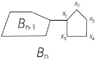
TYPE PENTACHAINSThe alpha-pentachains for n = 1 2, and n = 3 are depicted in Fig. 2. More generally, an
alpha-pentachain Bnwith n pentagons (see Fig. 3) can be obtained by attaching a pentagon,
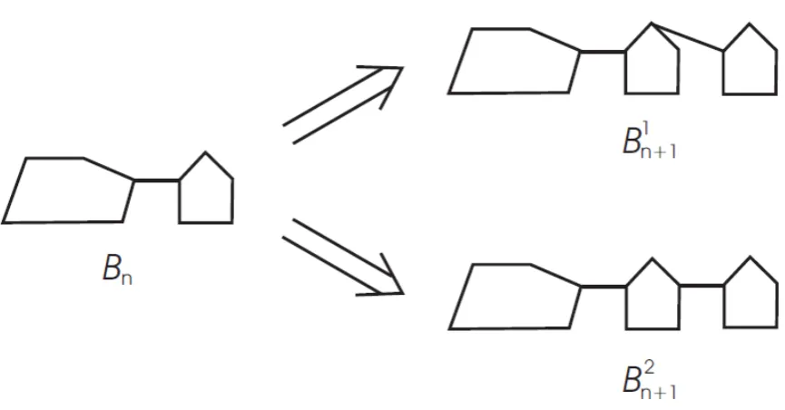
by means of an edge, to Bn−1 which has n −1 pentagons. However, for n ≥2, there are two
ways to arrange the terminal pentagon, leading to the local arrangementsB1n1 and Bn21as shown in Fig. 4.
Fig. 2. The alpha-pentachains with one, two, and three pentagons.
Fig. 4. The two types of local arrangements in alpha-pentachains.
Due to the random selection from Bk−1 to Bk , k = 3, 4, 5, . . . , we may regard an
pentachain obtained by stepwise addition of terminal pentagon as a random alpha-pentachain, denoted by Rn() if it has n pentagons, n > 2. Furthermore, at each step k = 3, 4, . . . , n, a random selection is emerged from one of the two possible constructions:
(1) Bk → B1k1 with probability p, and (2) Bk → Bk21with probability 1 − p. Here we
assume that the construction described is a zeroth–order Markov process, which means that the probability p is constant and independent of the step parameter k.
Denote by E(Ξ) the expected value of a random variable Ξ.
Theorem 1. For n ≥1,
. ) 3 25 2 5 ( ) 2 25 5 ( ) 5 15 ( 6 5 )) (
(W R( ) p n3 p n2 p n
E n (13)
Proof.As shown in Fig. 3, the pentachain Bnis constructed by adding a pentagon to Bn−1 by
means of a new edge. Based on this construction, it is easily to prove the following relations.
1◦. For any v ∈ Bn−1 ,
3 , 2 , 1 ,
) , ( ) ,
(x v d u 1 v k k
d k n
and
. 2 ) , ( ) , ( ,
3 ) , ( ) ,
(x4 v d u 1 v d x5 v d u 1 v
d n n
2◦. B
5
1
}. 5 , 4 , 3 , 2 , 1 { ,
6 ) , ( 3
i k i
k x
x d
Then we have
6 ) 1 ( 5 1 ) (
)
(x1B d u 1 B 1 n
d n n n (14)
6 ) 1 ( 5 2 ) (
)
(x2B d u 1 B 1 n
d n n n (15)
6 ) 1 ( 5 3 ) (
)
(x3B d u 1 B 1 n
d n n n (16)
6 ) 1 ( 5 3 ) (
)
(x4B d u 1 B 1 n
d n n n (17)
6 ) 1 ( 5 2 ) (
)
(x5B d u 1 B 1 n
d n n n (18)
and
W(Bn) = W(Bn−1) + 5d(un−1|Bn−1) + 55n −40 (19)
with the boundary condition W(B1) = d(u1|B1) = 15. Thus from (19), we obtain the recursive
relation
W(Bn+1) = W(Bn) + 5d(un|Bn) + 55 n + 15 . (20)
For a random chain Rn() , the distance number d(unRn()) is a random variable and we
denote its expected value by
)). (
( ( )
)
(
n n
n E d u R
U
There are two cases to be distinguished:
Case 1: Bn Bn11 . In this case, the vertex un coincides with the vertex labeled x2 or x5.
Then, d(un|Bn) is given by (15) or (18).
Case 2:Bn Bn21. In this case, the vertex un coincides with the vertex labeled x3 or x4 .
Then, d(un|Bn) is given by (16) or (17).
( ) 3 5( 1) 6
.) 1 (
6 ) 1 ( 5 2 ) (
) (
1 1
) (
1 1 )
(
n R
u d p
n R
u d p U
n n
n n n
(21)
Simplifying (21), the recursion formula for Un() becomes
9 5 ) 5 15 (
) (
1 )
(
p n p
U
Un n (22) with the boundary condition
6 2 1 2 1 ) (
( 1 1( )
) (
1 E d u R
U (23)
Eq. (22) combined with Eq. (23) provides the explicit expression of Un(), that is
. ) 3 5 ( 2 1 ) 5 15 ( 2
1 2
)
( p n p n
Un
By applying the expectation operator to equation (19), we get
15 55 )
3 5 ( 2 1 ) 5 15 ( 2 1 5 )) ( ( )) (
( ( 1) ( ) 2
E W R p n p n n
R W
E n n
with the boundary condition E(W(R1()))15. From the above recurrence relation, we arrive at Eq. (13), by which Theorem 1 is proven.
3
.
B
ETA-
TYPEP
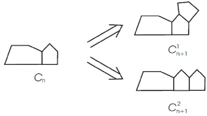
ENTACHAINSA beta-pentachain is a graph consisting of pentagonal rings, every two successive rings having a common edge, see Fig. 5. More generally, a beta-pentachain Cnwith n pentagons
(see Fig. 6) can be regarded as a beta-pentachain Cn−1 with n−1 pentagons to which a new
terminal pentagon {wn−1, vn−1, y1, y2, y3} has been adjoined. However, this terminal
pentagon can be added in two ways, resulting in the local arrangements described as C1n1
Fig. 5. The beta-pentachains with one, two, and three pentagons.
Fig. 6. A beta-pentachain with n pentagons.
Fig. 7. The two types of local arrangements in beta-pentachains.
process. Earlier, Rao and Prasanna considered the Wiener indices of beta-pentachains [14, 15]. In what follows, we provide an explicit formula for the expected value of the Wiener index of a random beta-pentachain.
Theorem 2. For n ≥1,
12 22 )
12 ( ) 2 (
) 2 6 ( ) 2 2 ( 3
2 3
3
2 1 1 1 1 1 1 0 1 ) (
1
n n
p n
p I
I c b a I b a I a Wn
(24)
with I0 , I1 , I2 , and I3 given in Lemma 1 whereas a1 , b1 , and c1 defined as
. 2 2 2 ,
3 2 7 ,
) 3 6 ( 2 1 ,
1 1 1 2 1 2
p a p p b p c p p
q
Proof. As seen from Figs. 5–7, the beta-pentachain is a graph consisting of pentagonal
rings, every two successive rings having a common edge. Taking into account this construction, we get the following basic relations:
1. For any v ∈ Cn−1,
d ( yk , v)=d ( wn-1 , v )+k , k=1,2 and d ( y3 , v ) = d ( vn-1 , v )+1 .
2. Cn−1 has 3n −1 vertices.
3.
3
1 2
3
1
. 2 ) , ( ,
} 3 , 1 { ,
3 ) , (
i i
i k i
y y d k
y y d
Then it is straightforward to establish that
3 ) 1 3 ( 1 ) (
)
(y1C d w 1C 1 n
d n n n (25)
2 ) 1 3 ( 2 ) (
)
(y2C d w 1 C 1 n
d n n n (26)
3 ) 1 3 ( 1 ) (
)
(y3C d v 1C 1 n
d n n n (27)
and
n C
v d C
w d C
W C
W( n) ( n1)2 ( n1 n1) ( n1 n1)12 (28) with the boundary conditions
. 0 ) ( ) (
)
(C0 d w0C0 d v0C0 W
Clearly, equation (28) implies
. 12 12 ) (
) (
2 ) ( )
(C 1 W C d w C d v C n
There are two cases to investigate:
Case 1:Cn C1n1. In this case, wn and vn coincide with x1 and x2 . Hence, d(wn|Cn) and
d(vn|Cn) are given by (25) and (26).
Case 2: Cn Cn21. In this case, wn and vncoincide with x2 and x3 . Hence, d(wn|Cn) and
d(vn|Cn) are given by (26) and (27).
If the expected values of d(wn Rn()) and d(vn Rn()) are denoted by,
respectively,
)) (
( ( )
)
(
n n
n E d w R
U and Vn()E(d(vn Rn()))
then the recursion formulas for Un() and Vn() are given by,
p n p U
n R
w d p n
R w d p U
n
n n n
n n
2 ) 3 6 (
6 ) (
) 1 ( 2 3 ) (
) (
1
) (
1 1 )
( 1 1 )
(
(30)
and
. 2 2 ) 3 3 ( )
1 (
2 3 ) (
) 1 ( 6 ) (
) (
1 )
( 1
) (
1 1 )
( 1 1 )
(
p n
p V
p pU
n R
v d p n
R w d p V
n n
n n n
n n
(31)
Meanwhile, from Eq. (29) we get
. 12 12 2
) ( )
(R(1) W R( ) U( )V( ) n
W n n n n (32) with the boundary conditions
. 0 ) (
) (
)
(C0() d w0C0() d v0C0() W
By applying the expectation operator to (32), and noting that
) ( ) ( )
(Un Un
E andE(Vn())Vn(), we get
12 12
2 ( ) ( )
) ( ) (
1
W U V n
Wn n n n (33)
where Wn()E(W(Rn())).
The aim of this subsection is to calculate the expected value of Wn() . To this end, usually
(31). Then, by making use of Eq. (33), one would arrive at the desired result. In what follows, instead of this usual way, we employ another direct approach to do so.
From Eq. (33) we conclude that Wn(1) can also be expressed as
). 1 2 1 1 ( 12 ) ( ) (
2 ( ) ( 1) 0( ) ( ) ( 1) 0( )
) ( 1 n n n V V V U U U
Wn n n n n
(34)
Hence, it remains to determine the values of the two sums in the bracket on the right–hand side of Eq. (34). Noting that U0() 0, by a direct calculation we find
n p n
p
Un )
2 1 3 ( 2 3 6 2 ) ( implying . 2 ) 2 1 3 ( ) 2 1 1
( 3 2
) ( 0 ) ( 1 )
( U U p n p n n
Un n (35)
On the other hand, Eq. (31) can be rewritten as
1 1 2 1 ) ( 1 )
( qV an bn c
Vn n (36)
where . 2 2 2 , 3 2 7 , ) 3 6 ( 2 1 ,
1 1 1 2 1 2
p a p p b p c p p
q
If we introduce an auxiliary quantity Hndefined by
) ( 0 ) ( 1 )
( V V
V
Hn n n
then Eq. (36) implies that Hnsatisfies the recursion relation:
. ) 2 6 ( ) 2 2 ( 3 ) 1 ( 2 ) 1 2 )( 1 ( 6 1 1 1 2 1 1 3 1 1 1 1 1 1 n c b a n b a n a H q nc n n b n n n a H q H n n n (37)
By virtue of Eq. (2) in Lemma 1, we obtain the following representation of Hn:
3 2 1 1 1 1 1 1 0 1 ) 2 6 ( ) 2 2 (
3 c I I
b a I b a I a
Hn (38)
where I0 , I1 , I2 , and I3 are defined in Lemma 1. Combining Eqs. (34), (35), and (38), one
4.
G
AMMA-
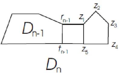
TYPE PENTACHAINSThe gamma-pentachains for n = 1,2, and n = 3 are depicted in Fig. 8. More generally, a gamma-pentachain Dnwith n pentagons can be obtained by attaching a pentagon by means
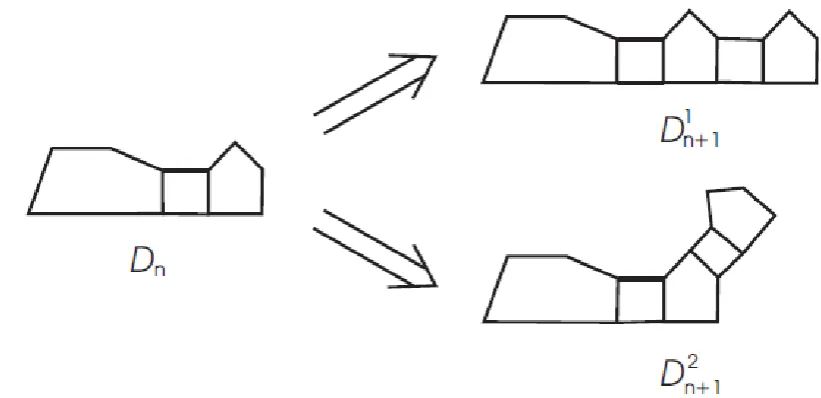
of two edges to Dn−1 which has n −1 pentagons (see Fig. 9). However, for n ≥2, three are
two ways to attach the terminal pentagon, leading to the local arrangements D1n1 and Dn21 shown in Fig. 10.
A random gamma-pentachain is constructed analogously to the above-described random alpha– and beta-pentachains.
Fig. 8. The gamma-pentachains with one, two, and three pentagons.
Fig. 10. The two types of local arrangements in gamma-pentachains.
Theorem 3. For n ≥ 1,
15 ) 2 5 39 ( 2 63
) 5 15 ( 2 1 2 ) 2 3
( ) (
3 2
2
3 3
2 2 2 2 1 2 2 0 2 ) (
1
n p n
n p I
I c b a I b a I a Wn
(39)
where I0, I1, I2, and I3 are given in Lemma 1and q, a2, b2, and c3 are given by
). 4 4 5 ( ,
10 2
23 2
15 ,
) 5 15 ( 2 1 ,
1 2 2 2 2 2 2
p a p p b p p c p p
q
Proof. As see from Figs. 8–10, the gamma-pentachain is a graph consisting of pentagonal
rings, every two successive rings connected by two edges. In view of this construction, we find the following basic facts:
1◦. For any v ∈ Dn−1,
d(zk, v) = d(rn−1,v) + k , k = 1, 2, 3 d(z4, v) = d(tn−1,v) + 2
d(z5, v) = d(tn−1, v) + 1 .
2◦. D
n−1 has 5(n −1) vertices.
3◦.
5
1
6 ) , (
i k i
z z
d , ∀k ∈{1, 2, 3, 4, 5}.
6 ) 1 ( 5 1 ) ( )
(z1D d r 1D 1 n
d n n n (40)
6 ) 1 ( 5 2 ) ( )
(z2 D d r 1D 1 n
d n n n (41)
6 ) 1 ( 5 3 ) ( )
(z3D d r 1D 1 n
d n n n (42)
6 ) 1 ( 5 2 ) ( )
(z4 D d t 1D 1 n
d n n n (43)
6 ) 1 ( 5 1 ) ( )
(z5D d t 1D 1 n
d n n n (44) and
W(Dn) = W(Dn−1) + 3d(rn−1|Dn−1) + 2d(tn−1|Dn−1) + 45 n −30 (45)
with the boundary conditions
W(D0) = d(r0|D0) = d(t0|D0) = 0 .
Replacing n by n + 1, we get from Eq. (45)
W(Dn+1) = W(Dn) + 3d(rn|Dn) + 2d(tn|Dn) + 45 n + 15 . (46)
There are two cases to be considered:
Case 1: DnD1n1 . In this case, rn and tn coincide with z2 and z3. Hence, d(rn|Cn) and
d(tn|Cn) are given by Eqs. (40) and (41).
Case 2: Dn Dn21 . In this case, rn and tn coincide with z3 and z4. Hence, d(rn|Cn) and
d(tn|Cn) are given by Eqs. (41) and (42).
If we introduce the notation
)) ( ( , )) ( ( ( ) ( ) ( ) ) ( n n n n n
n E d r R V E d t R
U
then we can obtain the following recursions for Un() and Vn() :
9 5 ) 5 15 ( 6 ) 1 ( 15 ) ( ) 1 ( 6 ) 1 ( 10 ) ( ) ( 1 ) ( 1 1 ) ( 1 1 ) ( p n p U n R r d p n R r d p U n n n n n n (47)
. 5 4 ) 10 5 ( ) 1 ( 6 ) 1 ( 10 ) ( ) 1 ( 6 ) 1 ( 15 ) ( ) ( 1 ) ( 1 ) ( 1 1 ) ( 1 1 ) ( p n p V p U p n R t d p n R r d p V n n n n n n n (48)15 45 2
3 ( ) ( )
) ( ) (
1
W U V n
Wn n n n (49)
with the boundary conditions
. 0
) ( 0 ) ( 0 ) (
0 V W
U
Noticing that Eqs. (47), (48), and (49) differ from Eqs. (31), (32), and (34) only by the coefficients, the remaining discussion and calculations follows closely the proof of the Theorem 2, and the final result, Eq. (39), is obtained in a similar way.
R
EFERENCES1. F. M. Brückler, T. Došlić, A. Graovac and I. Gutman, On a class of distance–based molecular structure descriptors, Chem. Phys. Lett., 503 (2011), 336–338.
2. F. Cataldo, O. Ori and A. Graovac, Wiener index of 1-pentagon fullerenic infinite lattice, Int. J. Chem. Model., 2 (2010), 165–180.
3. T. Došlić, A. Graovac, F. Cataldo and O. Ori, Notes on some distance–based invariants for 2-dimensional square and comb lattices, Iran. J. Math. Sci. Inf., 5
(2010), 61–68.
4. T. Došlić, A. Graovac, D. Vukičević, F. Cataldo, O. Ori, A. Iranmanesh, A. R. Ashrafi and F. Koorepazan Moftakhar, Topological compression factors of 2-dimensional rhombic lattice, Iran. J. Math. Chem., 1(2) (2010), 73–80.
5. R. C. Entringer, D. E. Jackson and D. A. Snyder, Distance in graphs, Czech. Math. J., 26 (1976), 283–296.
6. A. Graovac, O. Ori, M. Faghani and A. R. Ashrafi, Distance property of fullerenes, Iran. J. Math. Chem., 2(1) (2011), 99–107.
7. A. Graovac and T. Pisanski, On the Wiener index of a graph, J. Math. Chem., 8 (1991), 53–62.
8. I. Gutman, J. W. Kennedy and L. V. Quintas, Wiener numbers of random benzenoid chains, Chem. Phys. Lett., 173 (1990), 403–408.
9. H. Hosoya, Topological index. A newly proposed quantity characterizing the topological nature of structural isomers of saturated hydrocarbons, Bull. Chem. Soc. Japan, 44 (1971), 2332–2339.
11.M. Juvan, B. Mohar, A. Graovac, S. Klavžar and J. Žerovnik, Fast computation of the Wiener index fasciagraphs and rotagraphs, J. Chem. Inf. Comput. Sci., 35
(1995), 834–840.
12.O. Ori, F. Cataldo and A. Graovac, On topological modeling of 5/7 structural de fects drifting in graphene, in: M. V. Putz (Ed.), Carbon Bonding and Structures: Advances in Physics and Chemistry, Springer, Dordrecht, 2011, pp. 43–55.
13.O. Ori, F. Cataldo, D. Vukičević and A. Graovac, Wiener way to dimensionality, Iran. J. Math. Chem., 1(2) (2010), 5–15.
14.N. P. Rao and A. L. Prasanna, Wiener indices of pentachains, presented at National Conference on Discrete Mathematics and Its Applications, NCDMA 2007, Madurai, India.
15.N. P. Rao and A. L. Prasanna, On the Wiener index of pentachains, Appl. Math. Sci., 49 (2008), 2443–2457.
16.D. H. Rouvray, The value of topological indices in chemistry, MATCH Commun.
Math. Chem. 1 (1975) 125–134.
17.J. Sedlar, D. Vukičević, F. Cataldo, O. Ori and A. Graovac, Compression ratio of Wiener index in 2D-rectangular and polygonal lattices, Ars Math. Contemp., 7(1)
(2014), 1–12.
18.H. Wiener, Structural determination of paraffin boiling points, J. Am. Chem. Soc.,
69 (1947), 17–20.