Vol. 10, No. 4, 2018 Article ID IJIM-01034, 11 pages Research Article
Weak Disposability in Integer-Valued Data Envelopment Analysis
A. Amirteimoori ∗†, M. Maghbouli ‡
Received Date: 2017-02-26 Revised Date: 2017-10-22 Accepted Date: 2018-02-01 ————————————————————————————————–
Abstract
Conventional data envelopment analysis (DEA) models normally assume all inputs and outputs are real valued and continuous. However in most application- related problems some inputs and outputs can only take integer values, also, both desirable and undesirable outputs can be generated (e.g., the number of traffic accidents and deaths in a transportation system). In this paper the effect of undesirable outputs in integer DEA model is discussed. The proposed model distinguishes weak disposability of outputs imposing non-uniform abatement factor. Compared with radial models, a non radial model that directly deals with slacks is developed to calculate efficiency for integer-valued data set. An empirical application is used to illustrate the approach.
Keywords : Data Envelopment Analysis (DEA); Weak-Disposability; Undesirable factors; Integer-valued data; DMU; Efficiency.
—————————————————————————————————–
1
Introduction
F
o(DEA) has been serving as a methodology tor a long time, Data Envelopment Analysis evaluate the performance of various decision mak-ing units (DMU) that consumes multiple inputs to generate multiple outputs. Conventional DEA models have been created according to applica-tion, radial models as CCR (Charnes et.al [3]) and BCC (Banker et.al [1]) or non-radial models as SBM (Tone, [20]) and so on. These models take real-valued desirable inputs and outputs. A contribution of the conventional DEA model is that some of the input and/or output data are∗Corresponding author. [email protected], Tel: +(98)9113330785.
†Department of Mathematics, Islamic Azad University, Rasht Branch, Rasht, Iran.
‡Department of Mathematics, Islamic Azad University, Hadishahr Branch, Hadishahr, Iran.
characteristically integer- valued. Making use of categorical or ordinal data usually allows includ-ing integer-valued data into the analysis can be seen in articles such as Banker and Morey [2]; Kamakura [10] and Rousseau and Semple [18] among authors. The first DEA model allows explicit integrality constraints was developed by Lozano and Villa ([16],[17]). They proposed a mixed linear programming (MILP) DEA model which restricted the computed targets to inte-gers. However, as later argued by Kuosmanen and Kazemi Matin [11] this model does not com-ply with the minimum extrapolation principle (Banker et.al [1])which is the theoretical foun-dation of DEA models. Furthermore, the pro-posed model tends to overestimate the efficiency score. To address these issues, Kuosmanen and Kazemi Matin [14] developed an alternative pro-gramming problem with constant return to scale technology (CRS) based upon a new axiomatic
foundation of natural disposability and natural divisibility for production possibility set involv-ing integers. To be in line with different technolo-gies, the CRS framework was extended to other situations like variable, decreasing and non-increasing return to scale environments. Kuos-manen and Kazemi Matin [14] established a new notion of natural convexity, which restricts the feasible convex combination to the subset made up of integer-valued points, but the NDRS vari-ant requires a new postulate of natural augment-ability. The connection to NIRS technology is characterized by making use of the earlier nat-ural divisibility axiom. Recently, Kazemi Matin and A. Emrouznejad [11] introduced the notion of boundedness on the subset of output variables in an integer-valued DEA model in an axiomatic approach. Based on the new introduced axiom of ”outputs bounded scale,” the associated minimal extrapolation PPS is constructed. A mixed inte-ger linear programing (MILP) formulation similar to integer-valued DEA models was suggested for computing output efficiency scores of the units. In a paper presented by D. Khezrimotlagh on DEA conferences in 2015, committed that lin-ear integer DEA models does not mathemati-cally represent the Integer Production Possibil-ity Set (IPPS). Therefore, the benchmarking may not be appropriate. The paper was clearly eluci-dated this gap and the proposed model can re-move the gap. Also, the validity of the method is mathematically proved. A real-life application on university efficiency was examined to depict the differences of several integer DEA models in benchmarking decision making units. G. R. Ja-hanshahloo and M. Piri [9] proposed a modified model to evaluate the main units in the presence of negative integer data. First, the semi-oriented radial measure (SORM) based on negative data is depicted. After distinguishing the drawbacks of the model, the modified model is introduced, then the model reformed in presence of negative inte-ger values. On the other hand, in recent years, there has been serious attention to modeling un-desirable inputs/outputs in DEA literature. Fare et.al [6] developed a non linear DEA model uti-lizes Farrell -type of efficiency measure to simul-taneously increasing of desirable outputs and de-creasing the undesirable outputs by the same
slack results, directions for improvement are eas-ily obtained for each input and output measure. Equipped with proposed set of axioms, we gener-alize the method to the hybrid case where both real and integer valued inputs and outputs are present. Being able to distinguish weak dispos-ability in current context, the modified Russell measure of efficiency is proposed and a MILP for-mulation for computing is derived. The specifica-tion of weak disposability in this advocated model not only provide decision maker with better in-sight into the performance of peer DMUs but also help carry out further analysis for managerial de-cisions. The results are directly applicable to all areas of economics where activity analysis mod-els are employed. The remainder of this study is going to be unfolded as follows: the next section summarizes strategic concepts and previous DEA works, which are clearly related to this study. The weak disposability technology and integer-based DEA models are fully covered in this sec-tion. Section 3 describes in detail the concep-tual and mathematical framework to measure ef-ficiency under weak disposability assumption for a hybrid case where some of data sets are deemed to be integer while the others are not. An empir-ical application to a real case is represented in section??. The contribution is summarized with a conclusion.
2
Preliminaries
2.1 weakly disposable technology
In this section a brief aspect of weak disposability of outputs is introduced. Using the same notation of Kuosmanen [13] the input vector is denoted by
x= (x1, ..., xN)∈R+N , desirable or good outputs by v = (v1, ..., vM) ∈R+M and the undesirable or bad outputs by w = (w1, ..., wJ) ∈ R+J . Data for firmk∈ {1, ...K}is represented by the vector (vk, wk, xk) , the production technology is char-acterized by production set Y = {(v, w, x)|x ∈ R+N can produce (v, w)}, or alternatively, by the output setP(x) ={(v, w)|(v, w, x)∈Y}. Follow-ing Shephard [19], weak disposability of outputs is defined as if (v, w)∈P(x) and 0≤θ≤1 then (θv, θw)∈P(x), x ∈RN+. In case of variable re-turn to scale, the production technology satisfies
the following requirements:
A1) Envelopment: (vk, wk, xk)∈Y, k∈K.
A2) Weak disposability for good and bad outputs:
(v, w, x)∈Y,0≤θ≤1 then (`v,`w,x)∈Y.
A3) Free (strong) disposability of inputs and good outputs:
(v, w, x)∈Y,(α, β)∈RM++N, v≥β, ⇒(v−β, w, x+α)∈Y
A4) Convexity;Y is closed and convex.
Equipped with these sets of axioms, Fare and Grosskopf [7] have formulated weak-disposable technology in terms of single, scalar valued abate-ment factorθ as:
TF G=
{
(v, w, x)| ∑K
k=1θzkvmk ≥vm m= 1, ..., M
∑K
k=1θzkwjk=wj j = 1, ..., J
∑K
k=1zkxkn≤xn n= 1, ..., N
∑K
k=1zk= 1
zk≥0, 0≤θ≤1 k= 1, ..., K
}
(2.1)
Note that the variables z = (z1, ..., zk) are re-ferred to intensity weights. To allow for non- uni-form abatement factors across firms, Kuosmanen [13] denotes the abatement factor of firmkbyθk.
The author argued the empirical output set as
TK ={(v, w, x)|
∑K
k=1θkzkvmk ≥vm, m= 1, ..., M,
∑K
k=1θkzkwkj =wj j= 1, ..., J,
∑K
k=1zkxkn≤xn n= 1, ..., N,
∑K
k=1zk= 1,
zk≥0, 0≤θk≤1k= 1, ..., K}
(2.2)
Note that formulation (2.1) is a constrained case of formulation (2.2) imposing θ1 = θ2 = ... =
θk =θ.
In particular, the non linear above technology can be restated in an equivalent linear form with a simple substitution of Kuosmanen [13]
Then we must have
λk =θkzk, µk= (1−θk)zk
Rearranging the terms, the activity analysis tech-nology (2.2) can be rewritten as:
TK(L)={(v, w, x)| ∑K
k=1λkvmk ≥vm, m= 1, ..., M
∑K
k=1λkwjk=wj, j = 1, ..., J
∑K
k=1(λk+µk)xkn≤xn, n= 1, ..., N
∑K
k=1(λk+µk) = 1
λk, µk≥0 k= 1, ..., K}
(2.3)
The above formulation (2.3) is now a linear form and the right hand sides of the envelopment con-straints are faced up with scaling variables.
2.2 Integer-Valued DEA
In conventional DEA, each observed data is pre-sented by a pair of non negative input and output vector (Xk, Vk)∈R+N+M, k∈ {1, ..., K}. Lozano and Villa [16] assumed that some observed data of DMUs are integer and they partitioned the set of input variables as I = II∪IN I and the set of output variables as V = VI∪VN I, where II
and VI are the subsets of the corresponding di-mensions that must be integer while the others are not. Subsets II and IN I as well as VI and
VN I are mutually disjoint also |II|=p≤N and
|VI|=q ≤M. The authors proposed the follow-ing possibility set:
T = {
(ˆx,vˆ)|xˆk≥
∑K
k=1zkxki ∀i,
ˆ
vk≤
∑K
k=1λkvkr ,∀r,
ˆ
xk,ˆvk∈Z≥0, ∀i∈II,∀r∈VI
}
Kuosmanen and Kazemi- Matin ([14], [15]) pro-posed the axioms for the scope of integer-valued input-output variables as:
B1) Natural disposability:
(x, v)∈T, (α,β)∈ZN++M, y≥β ⇒(x+α, v−β)∈T.
B2) Natural divisibility:
(x, v)∈T, ∃λ∈[0,1], (λx, λv)∈Z+N+S ⇒(λx, λv)∈T.
B3) Natural Convexity:
(x, v),(x′, v′)∈Y ⇒
(˜x.v˜) =λ(x, v) + (1−λ)(x′, v′)
, 0≤λ≤1 (˜x,v˜)∈Z+N+M ⇒(˜x,˜v)∈Y
B4) Integrality:(x, y)∈T ⇒(x, y)∈Z+N+S
B5) Natural augment ability:
(x, v)∈T,∃λ≥1, (λx,λv)∈Z+N+M ⇒(λx, λv)∈T.
B6)Minimum Extrapolation: T is the intersection of all sets satisfying(B1)−(B5).
Based on the mentioned notations a hybrid setting involving both real and integer valued data set offers a generalized frameworks, which refers to hybrid integer DEA (HIDEA) model. The axiomatic foundation starting from free disposability(A2) and convexity (A4)of real val-ued variables(IN I, VN I) and corresponding ax-ioms of natural disposability(B1) and natural convexity (B3) of integer-valued variables, also axiom (A1) is jointly satisfied by all observed data, the following reference technology for the VRS case may be restated as:
THIDEA V RS =
(
xI vI
xN I vN I
)
; (xI, yI)∈Zp+q + ;
( xI
xN I
) ≥∑K
k=1z k
( xI
k
xN I k
) ; (
vI vN I
) ≤∑K
k=1zk
( vIk vN Ik
) ; ∑K
k=1z
k = 1, zk ≥0 ∀k
(2.4)
format proposed by Kuosmanen and Kazemi-matin ([14], [15]) as :
Min `−”(∑Sr=1s+ r +
∑N n=1s−n +
∑p n=1s
I n)
s.t vo
r+s+r =
∑K k=1z
kvk
r, r∈V
θxo
n−s−n =
∑K
k=1zkxkn, n∈IN I
˜
xn−s−n =
∑K
k=1zkxkn, n∈II
θxon−sIn = ˜xn n∈II
˜
xn∈Zp+ n∈II
zk≥0, k = 1, ...,K s+
r ≥0,
∀r∈O, s−n ≥0, ∀n∈I, sI
n≥0, ∀n∈II.
(2.5)
Symbol ε denote a non-Archimedean infinites-imal and variables s+r, s−n and sIn represent the non-radial slacks and ˜xn ∈ Z+p is the integer-valued reference points for inputs II. DM Uo is
efficient if the optimal value ofθequals one. It is worth noting that (HIDEA) model above distin-guishes between two input slacks. The first type denoted by s−n(n ∈ II) and s−n(n ∈ IN I) repre-sents the absolute differences between the con-vex combination ∑Kk=1zkxk
n(or
∑K
k=1zkxnk) and
the reference points θxon( or ˜xn), while the
sec-ond type sIn(n ∈ II) represents the absolute dif-ferences between the reference point ˜xn and the
projection θxon for integer -restricted inputs.
3
Weak
Disposability
with
Integer-valued DEA
The purpose of this section is to show how weakly disposable technology can be modeled whenever some inputs and outputs are restricted to be integer. Based on preceding notations, each feasible activity -which was characterized by a triple non negative input and output vector (vk, wk, xk) k = 1, ..., K can be rewritten as
x= (xI, xN I) v= (vI, vN I) andw= (wI, wN I).
Without a less of generality, xI(I ∈ II), vI(I ∈ VI) and wI(I ∈WI)are the dimensions satisfies
integrality assumptions (B4). Suppose that
|II|= p ≤ N,|VI|= q ≤ M and |WI|= α ≤ J. In order to deal with weak disposability in a systematic fashion in hybrid setting- involving both real and integer valued data- a revised set of axioms is needed. Commencing from free disposability of inputs and good outputs (A3), weak disposability of good and bad outputs (A2) and convexity (A4) for real-valued data (xN I, vN I, wN I), the corresponding axioms of integer-valued variables are proposed as:
B1) Natural disposability of inputs and good outputs:
(x, v, w) ∈ T,(α,β) ∈ ZN++M, v ≥ β ⇒
(x+α, v−β, w)∈T.
B2) Integer weak disposability for good and bad outputs:
(x, v, w) ∈ T, ∃θ ∈ [0,1],(x, θv, θw) ∈ Z+M+J ⇒
(x, θv, θw)∈T.
B3) Natural convexity:
(x, v, w),(x′, v′, w′) ∈ T(˜x,˜v,w˜) = λ(x, v, w) + (1−λ)(x′, v′, w′), 0 ≤ λ ≤ 1,(˜x,v,˜ w˜) ∈ Z+ ⇒
(˜x,v,˜ w˜)∈T.
B4) Natural divisibility:
(x, v, w) ∈ T, ∃λ ∈ [0,1],(λx, λv, λw) ∈
Z+N+M+J ⇒(λx, λv, λw)∈T
B5) Natural augment ability:
(x, v, w) ∈T,∃λ≥1,(λx, λv, λw)∈ Z+N+M+J ⇒
(λx, λv, λw)∈T
alternative variants of return to scale axioms. Equipped with these sets of assumptions, the hy-brid integer DEA (HIDEA) reference technology for the VRS case can be stated as:
TV RSHIDEA = x
I vI wI
xN I vN I wN I
;
(xI, vI, wI)∈Z+N+M+J,
xI ≥∑Kk=1zkxkn, n∈II,
xN I ≥∑K
k=1zkxkn, n∈IN I,
vI ≤∑Kk=1θkzkvkm, m∈VI
vN I ≤∑K
k=1θkzkvkm, m∈VN I
wI=∑Kk=1θkzkwjk, j∈WI
wN I =∑K
k=1θkzkwjk, j ∈WN I
∑K
k=1zk= 1
0≤θk≤1
zk≥0
(3.6)
The following theorem establishes the axiomatic foundation of this reference technology un-der revised sets of assumptions to the subsets (IN I, VN I, WN I) and (II, VI, WI) respectively.
Theorem 3.1 Production set TV RSHIDEA is the minimum extrapolation production possibility set if subsets (IN I, VN I, WN I) Satisfy axioms(A2−
A4) and subsets (II, VI, WI) satisfy natural dis-posability of inputs and good outputs (B1), in-teger weak disposability of good and bad outputs (B2′) and natural convexity (B3) also axiom (A1) is jointly satisfied by all observed data set.
Proof. It suffices to show that the axioms (B1), (B2′) and (B3) are simply integrality re-stricted cases of (A3), (A2) and(A4). More-over, the same intensity variable z apply to both subsets (IN I, VN I, WN I) and (II, VI, WI). The minimum extrapolation theorem for the case of
real-valued data (IN I, VN I, WN I) with axioms (A1 −A4) has been formally proved by Banker et.al [1], the case of (II, VI, WI) with axioms
B1, B2′ and B3 was proved in Kuosmanen and Kazemi-Matin[15].
In spirit of alternative return to scale specifica-tion in IDEA framework, the axioms of natu-ral divisibility (B4) and natural augment -ability (B5) along with other postulates can interpret NIRS and NDRS variants of IDEA technology respectively. Moreover, the multiplier θk used in this VRS technology enables the reduction of the level of bad outputs if accompanied by the reduc-tion of desirable outputs in the same proporreduc-tion across all firms. To linearize reference technology
TV RSHIDEA, the intensity weight of firm k can be partitioned into two components zk = λk+µk. Using this substitution from Kuosmanen [13] the production technology (3.6) converts into the fol-lowing linear form:
THIDEA V RS =
x
I vI wI
xN I vN I wN I
;
(xI, vI, wI)∈Z+N+M+J,
xI≥∑K
k=1(λk+µK)xkn, n∈II
xN I≥∑K
k=1(λk+µK)xkn, n∈IN I
vI≤∑K
k=1λkvmk, m∈VI
vN I≤∑Kk=1λkvkm, m∈VN I
wI=∑K
k=1λkwkj, j∈WI
wN I=∑Kk=1λkwjk, j∈W N I
∑K
k=1(λk+µK) = 1
λk, µk≥0
(3.7)
problem:
σ=M inN1+J[∑Nn=1θn+
∑J j=1φj
]
s.t ∑K
k=1(λ
k+µk)xk
n= ˜xn−s−n, n∈II
˜
xn =θnxon−sIn, n∈II
∑K k=1(λ
k+µk)xk
n=θnxon−s−n, n∈IN I
∑K k=1λ
kvk
m= ˜vm+s+m, m∈VI
˜ vm=vo
m+sIm, m∈VI
∑K k=1λ
kvk
m=vmo +s+m, m∈VN I
∑K k=1λ
kwk
j = ˜wj, j∈WI
˜
wj =φjwjoI −sIj, j∈WI
∑K k=1λ
kwk
j =φjwOjo, j∈W N I
∑K k=1(λ
k+µk) = 1
λk, µk ≥0
˜
xn,v˜m,w˜j∈Z+
φj≥1 j= 1, ..., J
0≤θn≤1 n= 1, ..., N
s−n, s+ m≥0
sI
n, sIm, sIj ≥0, n∈II, m∈VI, j∈WI.
(3.8)
The MILP formulation above measures the ef-ficiency score of firm 0 in terms of the abate-ment potential factor in integer and real val-ued inputs and outputs. Also, the constraint
φj ≥1 j= 1, ..., J and 0≤θn≤1 n= 1, ..., N
are the requirements for dominance. It is worth to note both data set exhibit that variable re-turn to scale (VRS) and the objective function
can be represented as N1+J[∑Nn=1θn+
∑J j=1µj
]
, the Russell-input and bad output measure of efficiency. So, the optimal value of model (3.8) is equal to the Russell efficiency measure defined with respect to theTV RSHIDEAreference technology. In essence, model (3.8) and its constraints im-posed both integer and real restrictions on inputs and undesirable outputs whilst weak disposability influences the output set. In terms of efficiency measurement, we scope on minimizing the poten-tial changes in inputs and undesirable outputs. Top of all in the context of discrete set of points, the evaluated DMU can be projected optimally close to the non -negative integer feasible point through solving MILP formulation above.
4
Application
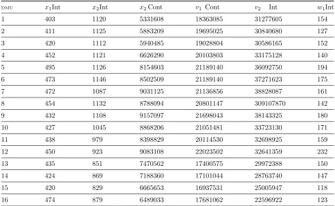
In order to see how weak disposability influences the hybrid output set, let us consider sixteen decision making units with three inputs which
is denoted by x1 and x2as integer valued and
x3as real-valued and four outputs. The last out-put componentw1 is characterized as undesirable one. w1 Is represented integer-values. The other componentsv1 and v2 are considered to be the number of desirable production. The first is inte-ger and the last indicates real valued. Table (1) summarizes all data set which was taken from Chen et.al [4]. In order to shed a light on pro-posed approach, the modified additive model in-troduced by Chen et.al [4] is recorded here. Again assume that, |II|= p ≤ N , |VI|= q ≤ M and
|WI|= α ≤ J. Also, according to the attributes the input vectorx= (xI, xN I) is categorized into desirable and undesirable integer-valued and real-valued. The notation xGn, xBn(n ∈ IN I) presents the real-valued input quantities and xGn, xBn(n ∈ II) depicts integer-valued desirable and
undesir-able inputs. Also the number of desirundesir-able and un-desirable integer-valued input sets can be shown as the index p1 and p2 with p = p1+p2. Based on preceding notations, the model has the format as follows:
ρ=M ax (N−p)+p 1
1+p2+q+(M−q)+α+(J−α)
× [∑
soGn − xGo
n
+soBn −
xBo n
+soGIn −
xGo n
+soBIn −
xBo n
+soIm+
vo m +
soN Im + vo
m +
soIj + wo
j +s
oN I+
j wo j ] s.t. ∑K
k=1λkxGkn =xnGo−soGn −, n∈IN I
∑K
k=1λkxBkn =xnBo+soBn −, n∈IN I
∑K k=1λ
kxGk n ≤x
Go n −s
oGI−
n , n∈I I
∑K
k=1λkxBkn ≥xnBo+soBIn −, n∈II
∑K
k=1λkvkm≥vmo +soIm+, m∈VI
∑K k=1λ
kvk m=v
o m+s
oN I+
m , m∈V N I
∑K k=1λ
kwk j ≤w
o j−s
oI+
j , j∈W I
∑K k=1λ
kwk j =w
o j−s
oN I+
j , j∈W N I
∑K k=1λ
k = 1
λk ≥0, k= 1, ..., K,
soG−
n , soBn −, soN Im +, s oN I+ j ≥0
soGI− n ∈Z
P1
+ , soBIn −∈Z P2 + ,
soI+ m ∈Z
q +, s
oI+ j ∈Z+α
Table 1: Efficiency Score and Dominance Factors.
DMU x1Int x2Int x2Cont v1 Cont v2 Int w1Int
1 403 1120 5331608 18363085 31277605 154
2 411 1125 5883209 19695025 30840680 127
3 420 1112 5940485 19028804 30586165 152
4 452 1121 6626290 20103803 33175128 140
5 495 1126 8154603 21189140 36092750 194
6 473 1146 8502509 21189140 37271623 175
7 472 1087 9031125 21136856 38828087 161
8 454 1132 8788094 20801147 309107870 142
9 432 1108 9157097 21698043 38143325 180
10 427 1045 8868206 21051481 33723130 171
11 438 979 8398829 20114530 32698925 159
12 450 923 9083108 22023502 32641359 232
13 435 851 7470562 17400575 29972388 150
14 424 869 7188360 17101044 28763740 147
15 420 829 6665653 16937531 25005947 118
16 474 879 6489033 17681062 22596922 123
In the above model, soGn − , soBn − ,soN Im +,soN Ij +
and
soGIn − ∈ZP1
+
,
soBIn −∈ZP2
+
,
soIm+∈Z+q
,
soIj +∈Z+α
are non-radial slack vectors of inputs and outputs of under evaluated DMU. Although the optimal value of the model does not depend on the units of measurement in inputs and outputs. Top of all, this additive model provides a closer on which variables cause a specific DMU to be inefficient by a certain amount. With these slack results, directions for improvements are easily obtained for each input and output measure. It is worth noting that the inequality is used in model (4.9) for integer-restricted inputs and outputs because the convex combinations for frontier DMUs are not necessarily integer-valued.
Therefore, xGon −soGIn −(n∈II),xBon +soBIn −(n∈ II), vom+soIm+(m ∈ VI) and woj −soj,(j ∈ WI) , the reference target for integer factors may or may not be equal to the their projections on the efficient frontier, but must be dominated by their convex combinations of frontier DMUs. To obtain an efficiency score between zero and one, let the optimal solution of the model is (λk∗, s∗noG−, s∗noB−, sm∗oN I+, s∗joN I+, s∗noGI−,
s∗noBI−, s∗moI+, s∗joI+) , the efficiency score of
DM Uo can be computed as below:
ρ∗o = 1− (∑
s∗noG− xGon +
s∗noGI− xGon +
s∗joI+ woj +
s∗joN I+ woj
)
(N−p)+p1+(J−α)+α
1 + (∑
s∗noB− xBon +
s∗noBI− xBon +
s∗moI+ vom +
s∗moN I+ vom
)
(M−q)+q+(N−p)+p2
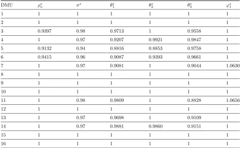
Table 2: Efficiency Score and Dominance Factors.
DMU ρ∗o σ∗ θ∗1 θ∗2 θ3∗ φ∗1
1 1 1 1 1 1 1
2 1 1 1 1 1 1
3 0.9397 0.98 0.9713 1 0.9558 1
4 1 0.97 0.9207 0.9921 0.9847 1
5 0.9132 0.94 0.8816 0.8853 0.9758 1
6 0.9415 0.96 0.9087 0.9393 0.9661 1
7 1 0.97 0.9081 1 0.9044 1.0630
8 1 1 1 1 1 1
9 1 1 1 1 1 1
10 1 1 1 1 1 1
11 1 0.98 0.9809 1 0.8828 1.0656
12 1 1 1 1 1 1
13 1 0.97 0.9698 1 0.9109 1
14 1 0.97 0.9881 0.9860 0.9151 1
15 1 1 1 1 1 1
16 1 1 1 1 1 1
model (4.9) are presented in the second column of Table 2. Applying linear program (3.8), the obtained efficiency score is presented in Table 2. When weak disposability is introduced, employ-ing the model based on technology (3.7) presents the following scores. The first column of Table 2
reports the efficiency score of the additive model (4.9) . Compared with the thirteen efficient units which were reported in model (4.9), the proposed approach records only eight efficient DMUs. For this application, the additive model (4.9) is not too helpful. Because model (4.9) considers un-desirable factors behaving like inputs. There-fore, in this computation effort through applying weak disposable assumption for undesirable out-puts the number of efficient unit decreases. It is worth to stress that the dominance factor which indicates weak disposability of undesirable out-puts and inout-puts play notable role in these results. The rest columns of Table 2 report the optimal values for non uniform dominance factors across all firms. As regards, the proposed formulations can be fallen beyond the scope of hybrid return to scale environments in efficiency measurement
contexts.
5
Conclusion
situations.
References
[1] R. J. Banker, A. Charnes, W. W. Cooper, Some models for estimating technical and scale inefficiencies in data envelopment anal-ysis, Management Science 9 (1984) 1078-1092.
[2] R. J. Banker, R. C. Morey, The use of cat-egorical variables in data envelopment anal-ysis, Management Science 32 (1986) 1613-1627.
[3] A. Charnes, W. W. Cooper, E. Rhodes, Measuring the efficiency of decision making units, European Journal of Operation Re-search 2 (1978) 429-444.
[4] Chien-M. Chen, J. Du, J. Huo, J. Zhu, Unde-sirable factors in integer-valued DEA: Eval-uating the operational efficiencies of city bys systems considering safety systems,Decision Support Systems 54 (2012) 330-335.
[5] K. H. Dakpo, P. Jeanneaux, L. Latruffe, Inclusion of undesirable factors in produc-tion technology modeling: The case of green-house gas emissions in French meat sheep farming, Working Paper SMART-LERECO 14 (2014) 1-47.
[6] R. Fare, S. Grosskopf, K. Lovell, C. Pasurka, Multilateral productivity comparisons when some outputs are undesirable: a non para-metric approach, The review of Economics and Statistics 71 (1989) 90-98.
[7] R. Fare, S. Grosskopf, Non parametric Pro-ductivity Analysis with Undesirable outputs: Comment, American Journal of Agriculture Economics 85 (2003) 1070-1074.
[8] R. Fare, S. Grosskopf, New Directions: Ef-ficiency and Productivity, Kluwer Academic Publishers,Boston, (2004).
[9] G.R. Jahanshahloo, M. Piri, Data Envelop-ment Analysis (DEA) with integer and neg-ative inputs and outputs,Data Envelopment Analysis and Decisions Science (2013) 1-15.
[10] W. A. Kamuraka, A note on the use of cat-egorical variables in data envelopment anal-ysis, Management Science 34 (1988) 1273-1276.
[11] R. Kazemi-matin, R. Emrouznejad, An Integer-valued data envelopment analysis model with bounded outputs, International Transactions in Operational Research 18 (2011) 741-749.
[12] D. Khezrimotlagh, Benchmarking decision making units with integer values in Data En-velopment Analysis, International Confer-ences on DEA in Economics and Finance, Technical University of Ostrava (2015).
[13] T. Kuosmanen, Weak disposability in non-parametric analysis with undesirable out-puts, American Journal of Agriculture Eco-nomics 87 (2005) 1077-1082.
[14] T. Kuosmanen, R. Kazemi-matin, Theory of integer-valued data envelopment analysis, European Journal of Operation Research218 ( 2009) 186-192.
[15] T. Kuosmanen, R. Kazemi-matin, Theory of integer-valued data envelopment analysis under alternative returns to scale axioms, Omega 37 (2009) 988-995.
[16] S. Lozano, G. Villa, Data Envelopment Analysis for integer-valued inputs and out-puts, Computers and Operations Research 33 (2006) 3004-3014.
[17] S. Lozano, G. Villa, Integer DEA models. In: Zhu, J., Cook, W. D., Modeling Data Irregularities and Structural Complexities in Data Envelopment Analysis, Springer, New York,(2007) 271-290.
[18] J. J. Rousseau, J. H. Semple, Categorical outputs in data envelopment analysis, Man-agement Science 39 (1993) 384-386.
[20] K. Tone, A slacks-based measure of effi-ciency in data envelopment analysis, Euro-pean Journal of Operational Research 130 (2001) 498-509.
Alireza Amirteimoori is a profes-sor in Applied Mathematics Op-erations Research group in Islamic Azad University in Rasht, Iran. His research interests lie in the broad area of performance man-agement with special emphasis on the quantitative methods of performance mea-surement, and especially those based on the broad set of methods known as data envelopment anal-ysis (DEA). Amirteimoori’s papers appear in journals such as International Journal of Math-ematics in Operations Research, IMA Journal of Management Mathematics, Applied Mathemat-ics and Computation, Journal of the Operations Research Society of Japan, Journal of Applied Mathematics, Expert Systems, Journal of Global Optimization, Decision Support Systems, Opti-mization, Central European Journal of Opera-tions Research, Expert Systems with Applica-tions, Transportation Research Part D: Trans-port and Environment, International Journal of Advanced Manufacturing Technology, RAIRO-Operations Research, Applied Mathematical Let-ters, International Journal of Production Eco-nomics, Measurement and the like.