Rapid Estimation of Water Flooding Performance and Optimization
in EOR by Using Capacitance Resistive Model
A.R. Bastami1, M. Delshad2, P. Pourafshary3
1- Graduate Student, Institute of Petroleum Engineering, University of Tehran 2- Graduate Student, Institute of Petroleum Engineering, University of Tehran 3- Assistant Professor, Institute of Petroleum Engineering, University of Tehran
Abstract
Water flooding, the oldest and most common EOR method, increases the displacement efficiency in a reservoir and also maintains the reservoir pressure for a long period of time. In Iran, water injection is widely used as a method to enhance recovery from oil reservoirs. Defining the optimized injection rates and injection patterns, dependent on the geological structure of the reservoir, is essential in operational and economical decisions for reservoir management.
In this paper, the Capacitance-Resistive Model is used to find interwell connectivity, and optimized injection rates in a synthetic field. In this approach, the reservoir receives injector rate variations as an input signal, while the producer responses determine the injector/producer pair connectivity quantitatively. This model is used to predict oil production for a specific reservoir, if the production/injection rate and bottomhole pressure data are available. The results show that the Capacitance-Resistive model has the capability to be used for the production history matching and to optimize the injection rate in different wells of a reservoir during the immiscible flooding to maximize the oil production. Moreover, they show that any change in oil and water prices can significantly influence the optimized water injection rates.
Keywords: Waterflooding, Water Injection, Production Forecast, Optimization, Capacitance Resistive Model
Corresponding author: [email protected] 1. Introduction
Oil recovery operations have traditionally been subdivided into three stages: primary, secondary, and tertiary. Historically, these stages described the production from a reservoir in a chronological sense. Primary production, the initial production stage, resulted from the displacement energy naturally existing in a reservoir. Secondary
recovery, the second stage of operations, was
usually implemented after primary
waterflooding (or whatever secondary process was used). Tertiary processes used miscible gases, chemicals, and/or thermal energy to displace additional oil after the
secondary recovery process became
uneconomical [1, 2].
2. Capacitance resistive model
The idea of this model is similar to the electrical current in the electrical circuits, including a network of capacitors and resistors. Hence, by considering flow stream, storage capacity in porous media, pressure difference and permeability similar to electrical current, capacitance, potential difference and resistance, respectively, the mathematical relations in electrical circuits can be used in the reservoir. In this model, a reservoir is supposed to receive a signal (injection) and deliver a reaction signal (production) to what it receives. Historical injection and production rates are the main input data for this model. Analyzing these data could provide a great deal of useful information about the reservoir and reduce the uncertainties in reservoir modeling. The final purpose is the economical and operational optimization in waterflooding projects to maximize the oil recovery [4]. Albertoni et al. used a simple model to find the interwell connectivity. He showed that even the injection rates of injectors which are far away from producers can affect their production rates. He estimated the interwell connectivity by a linear model and estimated
coefficients by using MLR1[5]. Yousef et al.
added a new parameter and developed the model to consider both capacitance and
1. Multiple Linear Regression
resistance effects by using compressibility and transmissibility concepts, respectively [6, 7]. Sayarpour et al. defined three different simplified models and presented analytical solutions for each and validated these solutions by applying them for some real fields [8, 9]. Weber et al. reviewed the problems of using this model in large scale fields with a large number of wells and suggested some solutions for minimizing the error caused by these problems [10]. Delshad et al. used this model to detect the presence of fractures in a reservoir and calculate the fracture permeability [11].
3. Mathematical developments
The material balance for a simple reservoir including one injector/producer pair as shown in Fig. 1, is as follows:
Figure 1.A control volume including one injector/ producer pair
t p dP
cV i ( t ) q( t )
dt (1)
To find an equation based on only injection and production rates, linear productivity index can be used.
) (P Pwf J
q (2)
By replacing average pressure form equation
(2) in equation (1), dt dP J t i t q dt
dq wf
() () (3)
where
is time constant. The solution of thisfirst order differential equation is as follows:
0 0 0 0 0 0 t t ( t t )
t
t t ( t t )
wf wf wf
t
e
q( t ) q( t )e e i ( )d J
e
P ( t )e P ( t ) e P ( )d
(4)This is the basic formulation of this model. Now, assume that the reservoir consists of different control volumes with a producer and 1 injector around it. [12]. A schematic representation of this approach is illustrated in Fig. 2.
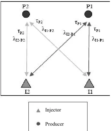
Figure 2. A schematic view of a reservoir with 2 injectors and 2 producers which describe the parameters of CRM in this modified approach.
In this approach, there is a time constant for
each producer and a weight coefficient for each pair of injectors and producers. Hence, the equations which describe the relations between injectors and producers are different in this approach:
dt dP J t i t q dt t
dq wfj
j i I i ij j j j
j
) ( . 1 ) ( 1 ) ( 1 (5)
where the time constant is defined as:
j p t j J V c (6)
The solution of the above equation is as follows: 0 1 0 0 0 1
( t t )
j j
t t I t t
wf , j
ij i j
i j
t t
j
j j j j
q ( t ) q ( t )e
dp
e e i ( )d e J e d
d
(7)Integration of the above equation leads to:
0 0
1
1
0 0
0
( t t ) I ( t t )
j j ij i i
i
t t I
wf , j i ij j i t j j j j
q ( t ) q ( t )e i ( t ) e i ( t )
dp di ( )
e e J d
d d
(8)By assuming that during the production intervals, the bottomhole pressure is varying linearly and the injection rates are constant, the describing equation would be as follows:
(5)
(6)
Injector
0 1 1 0 0 1 1 2
( t t )
j j
( t t ) t ( k )
n I
wf , j ( k )
ij i j j
k i k
j
k
j j
q ( t ) q ( t )e
p
e ( e ) I J
t j ( , ,...,I )
(9)4. Oil production model
To estimate the oil fractional flow in the production stream, an oil fractional flow model should be used in association with Capacitance Resistive Model. One of the suggested models is a power law relation between instantaneous water/oil ratio,Fwo,
and cumulative water injection rate, Wi [13].
Hence, the estimated water/oil ratio can be calculated from eq. 10.
i
wo W
F (10)
For a balanced system, total injection and total production are equal; hence, Wi is equal
to the total liquid production. This equation can be used for each well separately. By using eq.10 as the oil fractional flow model, we have: j j i j j wo wj oj wj oj oj
oj F W
q q q q q t f , , , 1 1 1 1 1 1 ) ( (11)
In this equation, cumulative water injection is as follows: ds s i ds s i
W inj Ninj
k t t k kj t t N
k kj k j
i [ ( ).] ( .)
1 1 , 0 0
(12)
where is the connectivity between an
injector/producer well pair or weight coefficient.
On the other hand, oil production rate from producer j is equal to the oil fraction,foj,
multiplied by total production, qj(t)as
follows: ) ( ) ( )
(t f t q t
qoj oj j (13)
The combination of eq. 11, eq. 12 & eq. 13 leads to the oil production rate from each producer:
1 0
1
1 2
j
oj N t
j kj k
k t
pro
inj
j
q ( t ) q ( t )
( i ( s ).ds )
( j , ,...,N )
(14)Hence, after estimating the CRM parameters (time constants & weight coefficients), the oil fractional flow parameters (j,j)
should be estimated by minimizing the difference between real and estimated values during history matching.
Since the direct application of eq. 10 in this form for finding model parameters is very difficult, a logarithmic form of this equation is suggested here.
) log( )
log( )
log(Fwo,j j j Wi,j (15)
By using a linear regression and minimizing the difference between real and estimated values, log(j)and j can be calculated.
This linear form of power law relation shows the limitations of using this model in
(13)
(14)
predicting oil production rate. In other words, this model can be applied if the logarithmic plot of water/oil ratio versus cumulative water injection is linear.
5. Optimization algorithm
The most important part of an optimization problem is determining the objective function. Depending on the purpose of the optimization, different objective functions can be defined. Some of these objective functions are as follows:
1. Maximizing cumulative oil production during a definite time interval
2. Minimizing cumulative water
production during a definite time interval
3. Maximizing net present value of the project by considering injection costs 4. Maintaining the oil production rate
from a specific field
Hence, the purpose of optimization can be to maximize ultimate oil production rate or to maximize the profit of the waterflooding in a reservoir. To maximize the profit of a waterflooding project during a specific time interval [t0,t], the suggested objective function is as follows:
pro Ninj
k t
t k w N
j t
t oj
o q s ds p i s ds
p R
1
1 0 ( ). . 0 ( ).
. (16)
where, poand pware oil and water price per
barrel, respectively.
Furthermore, decision variables are
production and injection rates. An upper and a lower boundary for injection through injectors can be defined according to the conditions of the reservoir.
The overall procedure of this optimization by using capacitance resistive model and oil fractional flow model is illustrated in Fig. 3. In this paper, the Microsoft Excel Solver is used to determine the CRM and fractional flow parameters. Moreover, it is used to solve the nonlinear mathematical equation to determine injection rates. Microsoft Excel Solver uses the Generalized Reduced Gradient (GRG2) Algorithm for optimizing nonlinear problems.
Figure 3. Workflow for the CRM application in history-matching and optimization [14]
6. Case study 6-1. 1*1 Model
0 1000 2000 3000 4000 5000 6000 7000 8000 9000
0 500 1000 1500 2000 2500 3000 3500
Ra
te
(b
bl
/d
ay
)
Time (day)
Injection Rate
Injection
Fig. 4.The injection rate versus time
Table 1.CRM parameters
τ λ q0,
RB/T
qtError,
RB/T
qtCorrelation
ratio P
1 0.5
9 1 15657 267 0.97
In Fig. 5, the real production rate is compared to the estimated production rate which is calculated by CRM. Hence, CRM is able to estimate liquid (water + oil) production rate accurately. In addition, by using CRM parameters we are able to forecast the production rate by accounting any change in the injection rate. In Fig. 6, the calculation procedure to find fractional flow model parameters (power low model) is illustrated.
0 1000 2000 3000 4000 5000 6000 7000 8000 9000
0 500 1000 1500 2000 2500 3000 3500
Ra
te
(b
bl
/d
ay
)
Time (day)
Production Rate
Real Estimated
Figure 5.The real production rate in comparison with estimated production rate
Using power low model parameters and selecting the desired objective function which is discussed in the previous section, injection rate optimization is possible. The
objective function in this study is to maximize the profit by considering the water injection cost equal to 1-3 $/bbl and different oil prices. In addition, the minimum and maximum limits of injection rate are supposed to be 0, 10000 bbl/day, respectively.
Figure 6. The graph of fractional flow model calculation
Table 2.Power low parameters
α β qoCorrelation ratio
6.412E-13 1.857 0.91
According to these results (Table 3, 4 & 5), if water injection costs 1$/bbl, for oil prices less than 18 $/bbl, water injection is not feasible. Also, if each oil barrel is worth $19, optimized water injection rate is equal to 5100 bbl/day. Finally, if each oil barrel is worth $20, optimized water injection rate is equal to 10000 bbl/day. These calculations for different water injection costs and oil prices are presented in the tables below.
Table 3. Optimized injection rate dependent on oil price, and water injection cost equal to 1 $/bbl
Oil Price ($)
Water Price ($)
Optimized Injection rate (RB/D)
18 1 0
19 1 5100
Table 4. Optimized injection rate dependent on oil price, and water injection cost equal to 2 $/bbl
Oil Price ($)
Water Price ($)
Optimized Injection rate (RB/D)
36 2 0
37 2 774
38 2 5100
39 2 9329
40 2 10000
Table 5. Optimized injection rate dependent on oil price, and water injection cost equal to 3 $/bbl
Oil Price ($)
Water Price ($)
Optimized Injection rate (RB/D)
55 3 0
56 3 2227
57 3 5100
58 3 7930
59 3 10000
6-2. 5*4 Model 6-2-1. Introduction
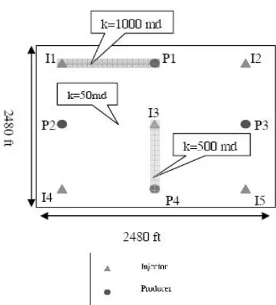
In this case, a synfield with 5 injectors, 4 producers and two high permeable streaks is considered. It is assumed that all the wells are vertical and they are perforated in all layers. The most important rock and fluid properties are presented in Table 6 and a schematic view of this reservoir is illustrated in Fig. 7. This model consists of 31*31*5 grids in X, Y and Z direction, respectively.
6-2-2. History matching
In this study, Capacitance Resistive Model parameters are used to forecast the production rate and to estimate the waterflooding performance quickly. In this case, 3051 days of operation in the form of 120 injection/production data are put into the model, and the model parameters, as presented in Table 7, are obtained after history matching.
Figure 7. A schematic view of a synfield with 5 injectors, 4 producers and two high permeable streaks
Table 6.Rock and fluid properties of 5*4 Model Value Parameter
80 X direction
Grid Size, ft Y direction 80
40 Z direction
0.18 Porosity, fraction
50 Permeability, md
2.0 Oil
Viscosity, cP
0.5 Water
5×10⁻⁶
Oil
Compressibility, psi-1 Water 1×10⁻⁶
1×10⁻⁶
Rock
Table 7.CRM parameters for 5*4 Model
Sum P4 P3 P2 P1 Parameters
0.566 2.517 5.324 0.503 τ
1 0.100 0.024 0.069 0.807 λ1j
1 0.246 0.198 0.034 0.522 λ2j
1 0.561 0.088 0.074 0.277 λ3j
1 0.520 0.062 0.202 0.217 λ4j
9.96 10.60 10.09 6.20 Error %
6-2-3. Production forecast
By using CRM parameters which are
obtained through history matching,
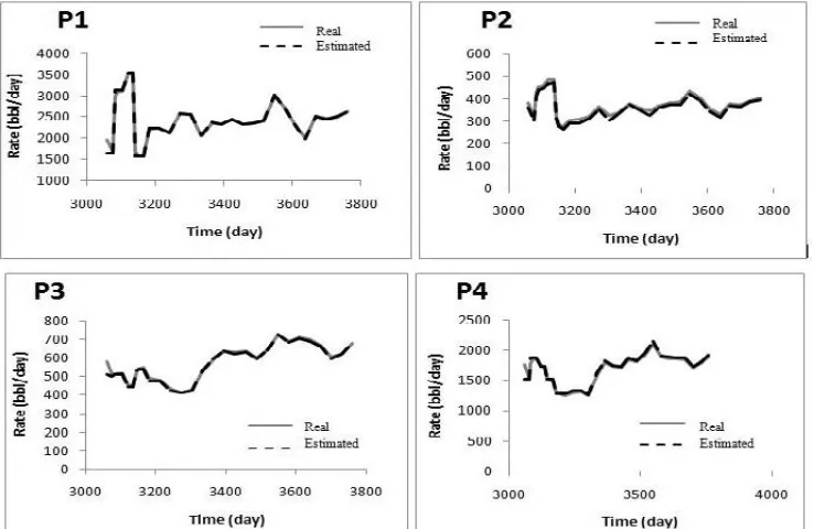
production has been predicted for 700 days. Hence, it is possible to study the capability of capacitance resistive model in predicting future production of the reservoir by comparing the predicted production rates with rates calculated by fine grid simulators (Eclipse). Fig. 8 shows the comparison between the values obtained by CRM and Eclipse for each producer. In this figure, “Real” represents the Eclipse results and the CRM results are shown as “Estimated”. The results show the estimated values of CRM are in agreement with the calculated values by Eclipse. Hence, CRM is capable of forecasting the future production even for reservoirs with more complexity and heterogeneities.
6-2-4. Optimization of the injection rates
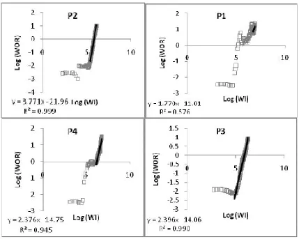
In this section, the calculation of injection rate optimization by using CRM is presented. Fig. 9 shows the oil fractional flow model (Power law) graphs in which parameters of models can be calculated for each producer and the interval that this model can be applied. Minimizing the error between estimated values and real values (like history matching) results in oil fractional flow model parameters, as it is presented in Table 8 for each producer.
Table 8.Estimated values for oil fractional flow model parameters
Wells
1.771 9.65E-12
P1
3.771 1.09E-22
P2
2.397 8.59E-15
P3
2.377 1.78E-15
Figure 9.The graphs based on power law model for estimating the fractional flow model parameters
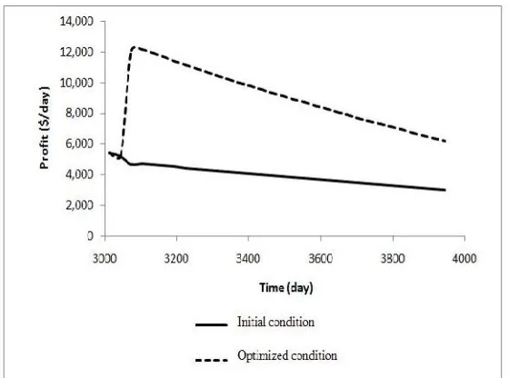
To optimize the injection rate, it is assumed that the rate of all injectors is constant and equal to the last value of the history for 30 months. Moreover, it is assumed that the minimum and maximum injection rates are 10 and 4000 STB/D, respectively. Thus, using CRM and fractional flow model parameters, with an assumption of 2 and 70 dollars cost per barrel for water and oil, respectively, the optimization based on maximizing the ultimate profit can be accomplished. Table 9 compares the rates of injectors before and after optimization. Using fine grid simulators provides us with a
measuring tool to compare the difference between production rates either by the initial injection rates or the optimized rates. This comparison for total production rate and profit is illustrated in Fig. 10 and Fig. 11, respectively.
Table 9. Comparison between the rates of injectors (bbl/day) before and after optimization
I1 I2 I3 I4 I5 InjectionTotal
Initial
rates 3001 1540 1291 963 1097 7892
Optimized
Figure 10.Comparison between the total production before and after optimization
Figure 11.Comparison between the profit before and after optimization
7. Conclusions
Nowadays, waterflooding is known as one of the most common EOR methods and also as a method to maintain the reservoir pressure in order to increase the ultimate oil recovery in the oil industry. Therefore, optimized water injection rate as an operational factor
that it is possible to calculate optimized injection rate by using this model for different reservoir and well geometries.
Nomenclature
Model coefficient Model coefficient
Weight coefficient
Integrating variable
Time constantt
c L2/F Total compressibility
wo
F Water/oil ratio
) (t
i L3/day Total injection rate
J L5/F-t Productivity index
P F/L2 Average pressure in the pore
volume
wf
P F/L2 Bottomhole pressure
) (t
q L3/day Total production rate
p
V L3 Pore volume
i
W L3 Cumulative water injection
Appendix
To derive the analytical solution of eq. 3, we first express the differential equation in a general form, or:
t r q dtdq
1 A-1
where,
dt dp J t i t r wf A-2This first-order differential equation can be generally solved by using the integrating factor technique. For this equation, the
integrating factor is given by:
t e dt etf 1 A-3
Then, by multiplying eq. A-1 by the integrating factor, or:
r t e q dt dqet t
1 A-4
it immediately follows that
r t e q e dtd t t
A-5
We now separate and integrate this equation with respect to t,
c e rt dt q
et t A-6
where c is the constant of the integration. By
dividing both sides by
t e ,
dt t r e e ceq t t t A-7
The constant of the integration c can be estimated by using the initial condition
tt0qt q t0
. Then Eq. A-7becomes,
dt t r e e e t qq tt0 t t
0 A-8
By substituting for r
t in the aboveequation, we get
0 0 0 t t t t wf t q q t edp
e e i J d
0 0 0 0 t t tt t t
wf
t t
q t q t e
dp
e e i d Je e d
d
A-9where, i is a variable of integration. The third term on the right of Eq. A-9 can be simplified by using integration by parts. The final analytical solution for Eq. 3 is,
0 0 0 0 0 0 tt t t
t
t
t t t
wf wf wf
t
e
q t q t e e i d
e
J p t e p t e p d
References[1] Latil, M., Enhanced oil recovery, 1st
edition, Technip, Paris, France, p. 1-2 (1980).
[2] Green, D. W. and Willhite, G. P., Enhanced oil recovery, SPE Textbook
Series VOL. 6, 2ndedition, Texas, USA,
p. 1 (2003).
[3] Bruce, W. A., "An electrical devices for analyzing oil reservoir behavior", Trans. AIME, p. 113-124, (1943). [4] Liang, X., Weber, D. B., Edgar, T. F.,
Lake, L. W., Sayarpour, M., and Yousef, A. A., "Optimization of oil production based on a capacitance model of production and injection rates", SPE 107713, Hydrocarbon Economics and Evaluation Symposium, Dallas, Texas, U.S.A (2007).
[5] Albertoni, A., and Lake L. W.,
"Inferring connectivity only from well-rate fluctuations in waterfloods", SPE Reservoir Evaluation and Engineering Journal, 6(1), 6 (2003).
[6] Yousef, A. A., Gentil, P., Jensen, J. L., and Lake, L. W., "A Capacitance model to infer interwell connectivity from
production and injection rate
fluctuations", SPE 95322, SPE Annual Technical Conference and Exhibition, Dallas, Texas, U.S.A. (2005).
[7] Yousef, A. A., Jensen, J. L., and Lake, L. W., "Analysis and interpretation of interwell connectivity from production and injection rate fluctuations using a capacitance model", SPE 99998, SPE/DOE Symposium on Improved Oil Recovery, Tulsa, Oklahoma, U.S.A. (2006).
[8] Sayarpour, M., Zuluaga, E., Kabir, C. S. and Lake, L. W., "The use of capacitance-resistive models for rapid estimation of waterflood performance", SPE 110081, SPE Annual Technical Conference and Exhibition, Anaheim, California, U.S.A. (2007).
[9] Sayarpour, M., Kabir, C. S., and Lake,
L. W. "Field applications of
capacitance-resistive models in
waterfloods", SPE 114983, SPE Annual Technical Conference and Exhibition, Denver, Colorado, U.S.A (2008). [10] Weber, D. B., Edgar, T. F., Lake, L. W.,
Lasdon, L., Kawas, S., and Sayarpour, M., "Improvements in capacitance-resistive modeling and optimization of large scale reservoirs", SPE 121299, SPE Western Regional Meeting, San Jose, California, U.S.A (2009).
[11] Delshad, M., Bastami, A. and
capacitance-resistive model for estimation of fracture distribution in the hydrocarbon reservoir", SPE 126076, SPE Saudi Arabia Section Technical Symposium, Khobar, Saudi Arabia, (2009).
[12] Bastami, A., The use of capacitance-resistive method for rapid estimation of immiscible flooding in enhanced oil recovery, M.Sc. thesis in petroleum engineering, University of Tehran, Iran, (2009).
[13] Gentil, P. H., The use of multilinear
regression models in patterned
waterfloods: Physical meaning of the regression coefficients, M.Sc. thesis in petroleum engineering, The University of Texas at Austin, Texas, (2007). [14] Sayarpour, M., Development and
application of capacitance-resistive
models to water/CO2 floods, Ph.D.
![Figure 3. Workflow for the CRM application inhistory-matching and optimization [14]](https://thumb-us.123doks.com/thumbv2/123dok_us/8887748.1823412/5.612.328.530.274.465/figure-workflow-crm-application-inhistory-matching-optimization.webp)