ISSN: 2333-6064 (Print), 2333-6072 (Online) Copyright © The Author(s). All Rights Reserved. Published by American Research Institute for Policy Development DOI: 10.15640/jfbm.v3n2a5 URL: http://dx.doi.org/10.15640/jfbm.v3n2a5
Modeling the Casual Link between Financial Development and Economic Growth in Sierra Leone
Isata Tarawally
1, Zhina Sun
2, Alimamy Amara Kargbo
3& Mohamed Kargbo
4Abstract
Slow growth has been the case in many Sub Saharan Africa (SSA) Countries in the 1970s and 1990s. The financial sector performance of most SSA countries in the 1990s to early 2000s has been dismally limited, with uneven reforms in the financial sector. This situation is the case for Sierra Leone; the financial sector performance is mixed and largely attributed to weak intermediation, inadequate legal and judicial environment, institutional and administrative bottlenecks in conducting banking and financial services. Given the role of finance on growth, this study investigates the link between financial development and economic growth in Sierra Leone from 1985-2010, using the Granger Causality test. This study shows that the overall financial depth and credit to the private sector have positive impact on growth. While, the interest rate spread and inflation negatively affect growth. The policy implication is that the real sector growth policy should be emphasized. Therefore, the government should strive to attain sound macroeconomic stability. This study contributes to current literature by providing an econometric understanding of relationship in finance and economic growth for SSA countries. This understanding is important for academics, policy makers and development organizations in shaping the future financial sector infrastructure and economic growth.
Keywords: Financial Development, Economic Growth, Sub Saharan Africa, Causality Test and Sierra Leone.
Introduction
The nature of the relationship between finance and economic growth has been one of the most debated in the recent past, yet with little consensus. Central to this debate is the question of whether strong economic performance is finance-led or growth driven. The question is because the determination of the causal pattern between finance and growth has important germane implications for policy-makers’ decisions about the appropriate growth and development polices to adopt. The fact that strong correlation exists between finance and economic growth has been well documented in the economic development literature.
However, previous empirical studies have produced mixed and conflicting results on the nature and direction of the causal relationship between finance and economic growth. Despite advances in the growth literature, the question as to whether financial systems play a causal role on economic growth remains an unsettled puzzle. Schumpeter (1969) argues that financial systems are important in promoting innovations and that economies with more efficient financial systems grow faster relative to those without. The view that the development of a country’s financial system fosters economic growth is consistent with the “supply-leading” view of the finance-growth relationship (Patrick 1966). The philosophy underpinning this view argues for the existence of a positive causal relationship flowing from financial development to economic growth. The “supply-leading” argument of the finance-growth literature states that the development of a viable financial sector is a pre-requisite for economic finance-growth.
1 Department of International Business and Management, Zhejiang Normal University (Jihua), China. 2 Department of International Business and Management, Zhejiang Normal University (Jihua), China. 3 Department of Finance, School of Economics, Jilin University, China.
It is generally believed that the financial system in Sub-Saharan Africa is relatively less developed and diversified compared to other regions of the world (World Bank, 1994). Sub-Saharan African countries lagged behind in all the measures of financial development when compared to the various regions of the world. The interest rate spread which measures the efficiency of financial intermediation is equally high compared to other regions. The two countries with single digit figure are Kenya and Nigeria. Until the implementation of the reforms in most African countries in the mid 80s, commercial banks dominated the banking system. These commercial banks were largely owned by the government.
It is important to note that the instability of the financial sector including banks offer important theoretical insights and policy recommendation that are particularly valuable in areas of the world suffering from banking and financial crisis and low level of domestic mobilization of capital for investment and economic growth. Consistent with this notion, on building a safe, sound and stable banking system and promote financial and economic growth, Sub-Saharan African region have suffered tremendously from low level of capital accumulation due to limited level of capital inflows, declining export receipt due to deteriorating terms of trade and mounting external debt leading to severe constraints on resources used for development of the banking sector and consequently posed difficulty of maintaining financial sector stability and economic growth. Flamimi et al., (2009)
Given the growing concern by African countries to improve on the poor growth episodes of the 1970s, development of the financial sector attracted considerable attention from policymakers across the continent. Since the mid-1980s, most African countries have experimented with policies of financial sector reforms partly motivated by the Structural Adjustment Programs (SAP) articulated by the World Bank and International Monetary Fund (IMF), as well as efforts to catch up with the pace at which other developing economies have been growing, particularly the East Asian Countries. The focus of the reform agenda in most of these countries aims at accomplishing extensive liberalization of interest rates, deregulation of the financial sector, strengthening the banking system, introduction of new financial instruments, and development of securities markets, particularly the stock market. Emphasis has also been placed on the establishment as well as the expansion of already existing stock markets in an effort to expedite domestic resource mobilization as well as attracting foreign capital so as to boost domestic investment and hence growth. World Bank (1994)
However, with the reforms in 1980s, new structure has started to emerge. The number of banks in the region has increased. As an illustration, the number of commercial banks increased from 213 in 1982 to 245 in 1992. In addition, government ownership of the bank has decreased significantly in most Sub-Saharan African (SSA) countries. Moreover, non-bank financial institutions have begun to play an increasingly important role in saving mobilization. However, owning to limited range of financial instruments and investment opportunities, their assets have typically been concentrated in government securities or deposited at banking institutions, where they have not been mediated for productive investment owing to banks’ limited lending operation and portfolio management. Most governments in SSA region embarked on financial sector liberalization in the mid 80s as their financial sector were highly repressed before the reform with selected credit controls and fixed interest rates (Gelbard and Leite, 1999)
This situation is the case for Sierra Leone, the banking sector dominates the financial sector and as such any failure in the sector has an immense implication on the economic growth of the country. The economy experienced moderate growth in the 1970s, and growth performance in the 1990s and 2000s was mixed. The poor performance of the economy is partly blamed to the ineffective functioning of the financial system as demonstrated by inadequate bank supervision, weak coordination among banks, inadequate payment system infrastructure and the subjective assessments of credit creation not consistent across banks and leading to high volume of non-performing loans and liquidity problem and impacts negatively on the financial sector and hence growth (Financial Sector Development Plan, 2009).
The Bank of Sierra Leone was now better placed to pick up early warning signals of weaknesses in the financial sector, because of this; commercial banks were able to survive the devastating events of the 1997 and 1998 rebel incursion. The regulatory and supervisory role was extended to other financial institutions, which led to the enactment of the financial services Act in 2010. One fundamental intermediation gap that requires attention, in the context of providing appropriate financing for poverty reduction is the lack of medium to long term lending facilities by commercial banks in particular (Bank of Sierra Leone Annual Report, 2011)
Despite the widespread financial sector reforms that have taken place, the financial systems in Sierra Leones exhibit some level of inefficiency, illiquidity, and thinness. Owing to widespread over-regulation of the financial systems, the country continues to experience high levels of capital flight. It is more imperative to gather theoretical and empirical ideas at a time when the nation has set its sight on growth and development; the financial sector development is one key area for growth and development (Sierra Leone Agenda for Change, 2008)
Now that growth promotion in the financial sector is being actively supported by the IMF, World bank, and other international institutions and the Government, all these effects requires research to find out how the growth in the financial sector would impact on the economic growth. The Sierra Leone economy provides a good test laboratory. Reliable and a long term time series data is available for Sierra Leone that allows for an econometric analysis to make reasonable conclusions about the relationship between financial development and economic growth. Studies thus, far have looked at some of the key determinants to sustained economic growth, but studies on how financial development can impact on the economic growth of developing country like Sierra Leone are scant.
Despite the introduction of the IMF and World Bank programs, growth in Sierra Leone has been bad. To address these issues, this study therefore, endeavors to carry out a systematic examination on the extent to which financial development has affected growth in Sierra Leone. Specifically, the study seeks to; (i) empirically determine the effect of specific measures of financial development on economic growth in Sierra Leone; (ii) examining the direction of causality between financial development and economic growth; and (iii) providing policy recommendations to academics, policy makers and development organizations in shaping the future financial sector infrastructure and hence economic growth. These specific characteristics of Sierra Leone’s growth process offer us the test case to investigate the link between financial development and economic growth in Sierra Leone, and are one of the motivations of this study.
Therefore, we propose the following hypotheses that can be tested. This is because hypotheses are statements that can be proven or disproven. Hence, we test the Null hypothesis against the alternative hypothesis thus; Null Hypothesis( ): There exist positive correlation between financial development and economic growth
Alternative Hypothesis( ): There exist negative correlation between financial development and economic growth : Causal relationship exists between financial sector development and economic growth in Sierra Leone
Alternative Hypothesis( ): Causal relationship does not exist between financial development and economic growth. The attempt to provide logical explanations on the above issues constituted major challenges of the current study. Data on annual growth variables such as Real Gross Domestic Product, and financial data on an annual basis such as Broad Money to GDP, Domestic Credit to the Private Sector by Banks, Interest Rates Spread, Real Exchange Rates, Inflation, Investment to GDP and Gross National Savings to GDP were collected from the International Financial Statistics, the World Bank, over the period 1985-2010. The Ordinary Least Square (OLS) regression estimation with the help of the Error Correction Model (ECM) technique is applied in the study. The Pair-wise correlation matrices are also applied to test the first hypothesis and the Granger Causality test is used to test the second hypothesis. E-views 6, software is applied in the analysis.
Analysis is therefore, restricted to a smaller number of variables than desired because of these restrictions. However, sufficient data is available for the purpose of this research.The rest of this paper is organized as follows: section 2 is literature review, followed by section 3, theoretical model and methodology. Section4 is results and discussions of the study. Finally, section 5 provides conclusion.
2. Literature Review
This section reviews the theoretical underpinnings and empirical literature in the context of developing and developed countries and to review a broader literature strand on the connection between financial development and economic growth. This understanding is crucial and important for carrying out an empirical analysis on the link between financial development and economic growth for the Sierra Leone economy.
2.1 Theoretical Literature
Available literature is presented between interest rates and economic growth, financial liberalization and economic growth and financial intermediation and economic growth.
2.1.1 Interest rates and Economic Growth
Policies of financial sector reforms were largely motivated following the financial repression argument popularized in the early 1970s by McKinnon (1973) and Shaw (1973) who underscored the appalling outcome of government failure in the financial sector. Advocates of the McKinnon-Shaw hypothesis argued that many financial systems in Africa have been subjected to financial repression characterized by low or negative real interest rates, high reserve requirements; mandatory credit ceilings; directed credit allocation to priority sectors; and heavy government ownership and management of financial institutions.
Financial repression refers to the distortion of domestic financial markets through measures such as ceiling on interest rates and credit expansion, selective allocation of credit and high reserve requirements, they pointed out that such misguided policies have damaged the economies of many developing countries by reducing savings and encouraging investment in inefficient and unproductive activities. The standard recommendation is then positive real interest is established on deposit and loans by eliminating interest rate ceiling, stopping selective credits allocation and lowering reserve requirements. The true scarcity prices of capital could then be seen by savers and investors leading to improved allocative efficiency and foster output growth.
On the other hand, Stiglitz (1993) observed that raising interest rates have favourable effects on financial intermediation and on growth. However, they noted also that excessively high real interest rates have adverse economic effects, this is the case extremely high interest rates will not permit the financing of investments projects that otherwise have good economic rational and will favour projects that have a high risk. The latter problem has become known as the heat of “adverse risk selection” on the assumption that risk tends to rise with the rate of return. 2.1.2 Financial Liberalization and Economic Growth
DornBusch and Reynoso (1989) underscored the importance of attaining macroeconomic stability prior to financial deepening. They noted that high and unstable inflation often increases the demand for financial deepening, but this might trigger further increases in inflation especially if fiscal deficits are large and the exchange rate is depreciating rapidly. As the government finances its deficits it will substantially reduced and the exchange rate stabilized before financial expansion is embarked upon.
Thus, the first phase of financial sector reforms in West Africa was characterized by the withdrawal of monetary authorities from directly interfering in the determination of lending and deposit rates of interest. As a result, commercial banks were given the freedom to set the lending and deposit rates on the basis of market conditions of demand and supply for credit.
2.1.3 Financial Intermediation and Economic Growth
Diamond and Dybvig 1993, noted that financial intermediaries are to provide liquidity to individual investors, unless financial intermediaries or financial markets exist, households can invest only in illiquid assets (for production). However, their precautions against an idiosyncratic liquidity shock might discourage them from investing in higher-yield, but more illiquid assets, financial intermediaries can reduce such inefficiency by pooling the liquidity risks of depositors and invest funds in more illiquid and more profitable projects.
Financial intermediaries can foster an efficient use of borrowed funds better than savers acting individually. Financial intermediaries can also improve managerial efficiency by promoting competition through effective takeover or threat of take over. Demirguc-Kunt and Maksimvonic (2005) argue that financial intermediaries and securities markets enable particular entrepreneurs to undertake innovative activity, which affects growth through productivity enhancement, and viewed financial intermediation as playing an important role in dampening the impact of external shocks on the domestic economy, concluding that financial systems without the necessary institutional development has lead to a poor handling or even magnification of risk rather than mitigation. These relationships provide the theoretical underpinnings for the current study
2.2 Empirical Literature
The next question concerns the empirical evidence of financial development and economic growth. Available evidence are presented on the relationship between interest rates and financial intermediation, between financial intermediation and economic growth and between financial deepening and economic growth
2.2.1 Interest Rates and Financial Intermediation
Lanyi and Saracogulu (1989) provide evidence on the relationship between interest rates and the growth of broad money supply (M2), measures as the real value of the sum of monetary and quasi-monetary deposits with the banking sector in a cross section relationship of 21 countries for the period 1971-1980 classifying countries according to whether they had positive real interest rates, moderates negative real interest rates or severely negative. The authors regresses the rates of broad money supply on interest rates. The results show a high correlation between the two variables with a regression co-efficient of the interest rate variable being statistically significance at the 1 percent level. In two similar approaches, Warman and Thirlwall (1994), and Athukorala (1998) arrive at rather opposite conclusions. For the case of Mexico over the period 1960 to 1990, Warman and Thirlwall (1994) find a positive impact of real interest rates on financial savings alone. Athukorala (1998) shows a positive impact of interest rates on all kinds of savings for India in the period 1955 to 1995, even though a weaker one for total saving (which includes the public sector). He is not able, however, to detect significant evidence for asset substitution as predicted by the neo-structuralists.
2.2.2. Financial Intermediation and Economic Growth
Bencivenga and Smith (1977) examines the relationship between the rate of growth of per capita GDP on one hand and the rate of growth of per capita real balances and the ratio of the broad money supply to GDP on the other hand. He found that the two variables representing the extent of financial intermediation were highly significant statistically in a cross-section regression for 67 developed and developing countries in 1967-1974. Romer (1986) found a positive relationship between real GDP and the real supply of domestic credit in a study of thirteen developing countries in a time series investigation, the credit available was statistically significant at the 1-percent level in the case of each countries.
However, Patrick (1966) suggested that the direction of causality changes in the course of economic development. In his view, financial development is necessary for sustained economic growth to take place but “as the process of real growth occurs the supply-leading impetus gradually becomes dominant” However, the existing empirical evidence, particularly by Odedokun (1996), has made significant progress in our understanding of the finance-growth linkage in Sub-Sahara Africa. Odedokun (1996) finds that aggregate measures of financial intermediation have positive and statistically significant effects on the growth rate of real per capita GDP.
2.2.3 Financial Deepening and Economic Growth
To understand the relationship between financial deepening and economic growth, researchers in recent time have also employed both firm-levels and industry-level data across a broad cross–section of countries in Europe and Latin America. These studies better addresses causality issues. For example, Demirguc-Kunt and Maksimvonic (2005) uses firm level data and financial planning model to show that developed financial system-as proxied by larger banking systems and more liquid stock markets-allow firms to grow faster than rates they can finance internally. Consistent with this study, Beck, et al (2008) also used firms level data in Asian countries of Indian, China and Bangladesh their results show that the sensitivity of investment to internal funds is greater in countries with less developed financial systems. Noting that financial deepening eases the obstacles that firms face to growing faster and that this effect is stronger particularly or small firms.
A good number of the empirical tests on the relationship between economic growth and financial development have often used broad money and private sector credit to GDP ratios as measures of financial sector development. For example, the World Bank (1994) has estimated that policies that would raise the M2/GDP ratio by 10% would increase the long-term per capita growth rate by 0.2–0.4% points. Arestis and Demetriades (2001) use measures like stock market capitalization (scaled by GDP) and report that stock markets have made significant contributions to growth in Germany, Japan, and France. In a study of 40 countries over the period 1978 to 1992, Mattesini (1996) uses the lending-deposit spread as a proxy for monitoring cost related to asymmetric information and find that the spread is particularly significant in explaining the growth performance for the whole sample and for the sub-sample of developed economies.
On balance, literature survey reveals that numerous studies have looked at the link between financial development and economic growth using a number of cross country approach; results of these studies are mostly inconclusive. These contradictory conclusions emerging from the empirical literature are one of the motivations for the present investigation. This study is different from most of the previous studies in the literature by examine the case of a typical Sub-Saharan Africa economy (Sierra Leone) that is structurally constrained and the financial sector climate still quite underdeveloped. Findings of the study contribute to theory by explaining the relationship between finance and economic growth. This is of important for policy makers who seek to develop policies for sustained financial infrastructure and economic growth. This understanding is also of significance for investors and businesses who seek to invest in profitable ventures for superior risk-adjusted returns.
3. Theoretical Framework and Methodology
A significant portion of the literature on development maintained that the extent of financial intermediation in an economy is an important determinant of its real growth rate. Following Bencivenga and Smith (1991), we pursue a modified version of the endogenous growth framework in specifying a model of growth that can account for the effects of finance in the growth process. This lends support for further use of econometric techniques capable of capturing the link between financial development and growth.
3.1 Theoretical Model of Finance and Growth
This section, however, develops a theoretical foundation to provide a more rigorous link between finance and growth. Here, the analysis is heavily draws from the contributions of the “endogenous growth literature” by Romer (1986). One of the many insights of this literature is that savings behavior will generally influence equilibrium growth rates. We assume a competitive economy with identical firms and households such that there is a coincidence between per firm and per capita values5.
We also assume that the stock of capital, Kt, at any point in time is made of both physical and human capital.
We let the aggregate level of output produced in the economy at time t,
Q
t to follow a linear function of theaggregate capital stock (Kt) as follows:
Q
t
K
t (1)Where
, the approximate state of technology or the rate of transformation of capital input into output. We assume further that, even though each of the N firms in the economy faces a constant returns to scale technology, productivity is however an increasing function of the stock of capital Kt . On the basis of this assumption, we assumethat each firm’s output is given as follows:
qt Kt
(2)
Where
q
t is firm-specific output,K
t is firm-specific capital stock and is a parameter that responds to thecapital stock 1 t K
. In this framework, we further assume that the stock of physical capital depreciate at the rate of
per period. Thus, gross investment, which is defined as the rate of growth of the capita stock (after adjusting for capital depreciation) is given as:
I
t
K
t1
1
K
t (3)Assuming a closed economy with no government intervention, a necessary condition for capital market equilibrium dictates that gross savings (S) equal gross investment. However, since a proportion of savings
1
leaks from the process of financial intermediation, capital market equilibrium requires thatI
t
S
. Hence1
1
From the aggregate production function in equation (1), the growth rate of output in period t +1 is given as:
1
1 t
1
t t
Y
g
Y
11
t tK
K
(4)By re-arranging equation (3), we have
I
t
K
t1
1
K
t Thus, by substituting for
1
1
t t t
K
I
K
in equation (4) above, we have;
1
t t t t t
t
t t
I K K K I
g K K
(5)Again, re-arranging equation (1), we have t Q K
now, by substituting for
K
t in equation (5) above, thegrowth of output at time t+1 becomes:
By invoking the capital market equilibrium condition that
I
t
S
t then equation (6) reduces to:
1
t
S
g
Q
(7)The steady state solution can then be deduced from equations (6) and (7) to obtain:
t
I
g
Q
(8)Where
S
Q
( i.e the saving rate) . In the context of the endogenous growth framework (Pagano, 1993; and Barro, 1989a), equation (8) predicts that financial development affects growth by either raising
or accelerating the social productivity of capital
; or it can influence the saving rate
.3.2 Methodology
3.2.1 Unit Root Tests:
When using time series annual economic data, it is important to note that most time series data are non-stationary which implies that the mean, variance and covariance of each variable is time variant otherwise the series is stationary. Hence using the OLS technique may imply that the result obtained would be spuriousi in the sense that the
variables may seem to have causation when there is no causation and the regression is meaningless. However, to overcome this notion, time series data requires being de-trended in a regression analysis. Thus we apply the idea of differencing for stationary at certain level or order, co-integration between non-stationary series require both series to be of the same order of integration. If a series is level stationary, we denote I (0) and stationary at first difference, we denote I (1), the series is integrated of first order. In general an I(d) process is a series that is stationary after differencing d-times (Hannan and Quinn, 1979).
We test for unit root of the series using the Augmented Dickey-Fuller (ADF) unit root test and the Phillip-Perron (PP) unit root test. The ADF is a test of the null hypothesis that the series are non-stationary I(1) against the alternative hypothesis that the series are- stationary I(0). The Philip-Perron (PP) test is also applied, which makes no assumption about the heteroskedascity and auto-correlated disturbances and suffers less from distribution issues and also adjust for the problem of endogeneity of the regressors. The ADF and PP tests have the same null hypothesis that unit root exist. Dickey and Fuller (1979) and (Phillips and Perron ,1988) The Augmented Dickey Fuller (ADF) test regression of a unit root is given by
t t 1 i t 1
x
μ βt
δx
δ x
δ
mx
tm
t
(9)
t t 1 i t 1
x
μ
δx
δ x
δ
mx
t m
t
(10)
Equation (9) contains a trend term, while equation (10) does not contain a trend time, and the lag terms are introduced in the model as additional regressors to account for heteroskedasticity and auto-correlation. But for the Phillip Perron, the lag m, is omitted to adjust for the standard error in order to correct for auto-correlation, heteroskedascity and problem of endogeniety. Thus, the PP test equation is specified as:
x
t
μ βt
δx
t 1
δ x
i
t 1
δ
m
x
tm
t (11)Null Hypothesis
H :
0δ
0
, the series has a unit root (non-stationary) that is I(1) against the Alternative HypothesisH :
1δ<0
the series has no unit root ( Stationary) that is I(0), if the calculated value of the tests statistic is lessthan the critical value at 0.05 of one tailed test, we rejectH
0 and acceptH
1. That is the series is I (0), stationary otherwise the series is I(1), non-stationary.3.2.2 Co-integration Tests
It is important to note that, if the series is stationary at differencing, conclusion made regarding information about the variables in the regression can only be valid for short run dynamics, while in the long run considerable and useful information would have been lost. To overcome this problem, we test whether the dependent variable exhibit long run equilibrium-relationship with the explanatory variables or are co-integrated using the Co-integrating Regression Augmented Dickey–Fuller (CRADF) test. This test uses residuals form of a co-integration regression, we estimate the model using OLS estimation by minimizes the sum of the squares residuals, Engel and Granger in Econometrica (1987) considers this test as one of the preferred test of co-integration and became known as Co-integration Regression Augmented Dickey Fuller (CRADF) test. The Co-Co-integration Augmented Dickey Fuller (CRADF) test regression equation is given by
e
t
1e
t1
1
e
t2
m
e
t m
t (12)From equation (12)
e
terms are included to eliminate any autocorrelation so that
2 tμ ~IID 0, δ
, notice that there is no constant in the regression. A constant can be included in either the co-integrating regression or the CRADF but not both. With a constant in the co-integrating regression equation, the residuals have zero mean, we do not expect the residuals to have a deterministic trend and so linear trend is not included.(Mackinnon, 1991),we carry the CRADF test thus:
0 1 t
H :
α
0 and e are I 1 , the series are not co-integrated
1 1 t
H :
α
0 and e are I 0 , the series are co-integrated
The test statistics under the null has no standard distribution, if the calculated value of the test statistic is lessthan the critical value then the null hypothesis of no co-integration is rejected; the series are co-integrated, m is the number of lagged terms is selected in the same way as for the unit root tests. We use Mackinnon (1991) critical values to make a decision on the test statistic and not the individual unit root values of the ADF test.
3.2.3 The Error Correction Model (ECM)
To ensure that the regression model is not spurious, we difference the series and following the Granger Representation Theorem (1987), we expressed a general ECM of the form
1
0 1
1
i 1
ln y
α
σ
ln X
τ
ln Y
ln X
γEC
ε
p p
i i t i t i t
i i
t i t
(13)
Where
ε
t is white noise, and γis the coefficient of the error correction term (EC ) which measures the3.2.4 Correlation Matrices
The pair-wise correlation matrices is applied to test for the existence of correlation between financial development and economic growth and to also determine the existence of multi-colinearity among the variables. 3.2.5 Granger Causality Test:
Causality is an important concept in empirical analysis and refers to the ability of one variable to predict or cause the other. The Granger (1969) causality procedure is developed to test for causal relation. According to Granger, Y causes X if the past values of Y can be used to predict X more precisely then simply using the past values of X and vice versa. Therefore, the relevance of this test is to determine the direction of causation between two variables(X and Y) in a time series data. The idea behind this test is to run the following bi-variate regression models, if we want to determine the direction of causality between X and Y
0 1
1 1
t t
X
γ
δ X
in m
t i t
i j j j
Y
(14) 2 1 t 1 0 iX
t in m t t i j j j
Y
Y
(15)
Where m and n are the number of lagged, X and Y are the terms respectively.
1t,
2t are the random errorsand follows
20,
N
equation (14) predicts that
X
tis related to past values of itself as well as that ofY
tand equation(15) predicts similar trend for
Y
t.If we want to test whether X Granger cause Y or/and Y Granger cause X we carryout an F-test on the joint significance of
jand
i respectively. Therefore, we proceed thus;
0 0
1 1
0 0
: j : i
m m
j i
and H
H
, respectively test thus:
We reject the
H
0,if the calculatedm n k
F F (k is the number of parameters estimated in equations (14) and
(15), n is the number of observations. Otherwise we do not reject
H
0.We may also use the Probability value of the F-statistic to make a decision based on the significance level, usually 1%, 5% and 10% respectively.3.3 Model Specification and Data Description
Given the increasing empirical evidence in support of the positive role of financial sector development in the growth process, we therefore modify equation (8) above by factoring in financial factors into the growth equation. Thus, by controlling for non-financial factors that influence long run growth6, we generalize the specification of a
growth equation that accounts for the effects of financial development.
According to Barro (1989a), the growth of real GDP is considered to depend on several variables. For the purpose of our study, the relationship between finance and growth can be augmented from the Barro-growth regression of financial development variables which takes the form thus;
Growth = α + β[Finance] + γ[conditioning set] +µ (16)
Where βthe coefficient of the measures of financial sector development/indicators and γ is the coefficients of the set of control variables.µ istheerroterm However, it is difficult to identify proxies for measuring financial sector development and growth. For instance, Beck et al., (2008) discuss different indicators of financial development capturing the size, activity and efficiency of the financial sector, institutions or markets.
6 The traditionally based neoclassical theory of growth has been focusing only on physical capita and labour inputs as the
However, this study improves on their models by including the Interest Rates Spread (IRS) on deposits and loans. However, financial markets development in Sierra Leone is still limited and thus available data is non-existence for the study period. In this study, our measures of financial development indicators are purely banking. Therefore, the selection of banking development indicators as appropriate proxies to financial development (FD) justifies the choice of financial development in Sierra Leone. This study therefore uses three financial development indicators mainly banking development indicators and includes broad money, domestic credit to the private sector by banks and interest rate spread.
The regression model is therefore specified with the Real GDP (RGDP) as dependent variable, measured as GDP growth on an annual basis adjusted for inflation. The explanatory variables comprise both the financial sector indicators and the control variables as follows:
Financial Sector indicators
The overall financial depth of the financial system (measured as the ratio of broad money to GDP, ie 2 M GDP )
Credit to the private sector by banks as a share of GDP, which is the value of loans made to the private
enterprises and households used as a measure of financial sector development. (i.e DCP GDP)
The interest rate spread is calculated as the difference between the deposit and lending rates and measures the degree of competitiveness/ efficiency in the banking sector, denoted as (IRS)
The Control/Conditioning variables include;
RER = Annual real exchange rate
INF= inflation, which is the average consumer prices, it measures the degree of uncertainties about the future market environment.
INV/GDP = Investment as a share of GDP ( measured as gross fixed capital formation)
GNS/GDP= Gross National Savings as a share of GDP
Hence,
2
, ,
M DCP
FD f IRS
GDP GDP
(17)
From equations 16 and 17, we specify our model for this study thus;
2
1 2 3 1 2
3 4
ln(RGDP) ln( ) ln( ) ln(IRS) ln( ) ln(INF)
ln ln( ) t (18)
M DCP
RER
GDP GDP
INV GNS
GDP GDP
1
<0 or>0,
2 <0 or>0,
3 <0,
1 <0,
2 <0,
3 <0 or >0 and
4 >04. Results and Discussions
Table 1: Present the Summary Statistics
Variables LNRGDP LNM2 LNDCP LNIRS LNRER LNINF LNINVT LNGNS
Mean 6.9 27.3 11.74 25.2 24.88 14.6 27.21 20.9
Maximum 214.4 336.3 209.5 315.5 624.1 476.3 112.3 225.9
Minimum 4.76 2.29 0.43 1.10 4.51 1.11 -3.69 -1.46
Std. Dev. 16.3 2.64 3.89 4.22 3.88 11.6 5.29 9.96
The summary statistics is performed on the natural logarithm of the data series of all the observed variables: Max= Maximum, Min=Minimum and Std. Dev=Standard Deviation. M2, DCP, INVT and GNS are in a ratio of GDP
The summary statistics reported in table 1, above indicates that on average Real Gross Domestic Product (RGDP) is 6.9 percent. The ratio of Broad Money (M2) to Gross Domestic Product (GDP) averaged around 27.3 percent, credit to the private sector by banks as a ratio of GDP stood at 11.74%, inflation averaged around 14.6%, the real exchange rate and investment (INVT) as a ratio of GDP average around 24.88% and 27.21% respectively. Interest rate spread stood at average 25.2 and gross national savings averaged around 20.9%. The double digit inflation rate (14.6%) observed from the summary statistics demonstrates an indication of macroeconomic instability, there is also high interest rate spread of around 25.2% which also clearly manifest low competition in the banking sector. The broad money which is the depth of financial deepening (27.3%) reveals that a high proportion of the financial assets are held outside the formal banking sector. Despite a positive value of the level of gross national savings (20.9%), and the credit to the private sector (11.74%), but are still considered low and thus demonstrates the underdeveloped nature of financial intermediation in the Sierra Leone economy. The overall investment as a ratio of GDP is low (27.21%), indicating that greater proportion of income is directed towards consumption and thus affect long term economic growth.
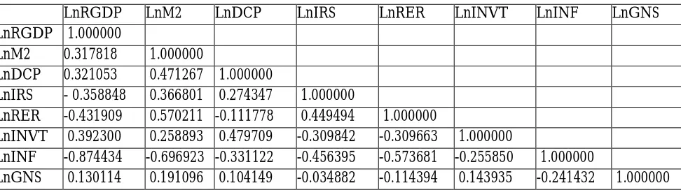
Table 2: Correlation Result
LnRGDP LnM2 LnDCP LnIRS LnRER LnINVT LnINF LnGNS
LnRGDP 1.000000
LnM2 0.317818 1.000000
LnDCP 0.321053 0.471267 1.000000
LnIRS - 0.358848 0.366801 0.274347 1.000000
LnRER -0.431909 0.570211 -0.111778 0.449494 1.000000
LnINVT 0.392300 0.258893 0.479709 -0.309842 -0.309663 1.000000
LnINF -0.874434 -0.696923 -0.331122 -0.456395 -0.573681 -0.255850 1.000000
LnGNS 0.130114 0.191096 0.104149 -0.034882 -0.114394 0.143935 -0.241432 1.000000 The correlation matrix is performed on the natural logarithm of the data series of all the observed variables. M2, DCP, INVT and GNS are in a ratio of GDP
Table 3: Result of the Augmented Dickey Fuller (ADF) Unit Root Test
Variable
Augmented Dickey Fuller (ADF) Unit Root Test
One-lag model Two-Lag Model Conclusion
Constant Constant and TrendConstant Constant and Trend
lnRGDP level -2.783530 -3.975549 -2.783530 -3.975549 I(1)
first difference -8.528265** -8.465620** -8.528265** -8.465620**
lnM2 level -2.445839 -2.113429 -2.445839 -2.113429 I(1)
first difference -5.155255** -6.337865** -5.155255** -6.337865**
lnDCP level -0.887271 -1.058828 -0.887271 -1.058828 I(1)
first difference -5.889944** -6.873239** -5.889944** -6.873239**
lnIRS level -3.5615865 -3.534759 -3.5615865 -3.534759 I(1)
first difference -7.916620** -8.460341** -7.916620** -8.460341**
lnRER level -4.544354 -4.734123 -4.544354 -4.734123 I(1)
first difference -5.250599** -4.789106** -5.250599** -4.789106**
lnINF level -1.612433 -1.463089 -1.612433 -1.463089 I(1)
first difference -11.26923** -11.24401** -11.26923** -11.24401**
lnINVT level -0.969294 -1.976895 -0.969294 -1.976895 I(1)
first difference -5.867742** -6.153552** -5.867742** -6.153552**
lnGNS level -3.870638 -4.004973 -3.870638 -4.004973 I(1)
first difference -5.979923** -5.902304** -5.979923** -5.902304**
** denotes 5% significance level respectively, and I (1) means order of integration. M2, DCP, INVT and GNS are in a ratio of GDP
The ADF unit root test is performed under the null hypothesis that unit root exist against the alternative hypothesis that unit root does not exist. The ADF unit root test in table 3, above shows that all the variables are not stationary in level but stationary at first difference, implying that all the variables are integrated of order one, denoted as I(1). The constant and the constant with trend for both one lag model and two lag models does not change the result of the ADF test. This implies that the time trend is not significant and can be dropped. But dropping it requires caution; therefore it is logically to remain in the regression output of the ADF test.
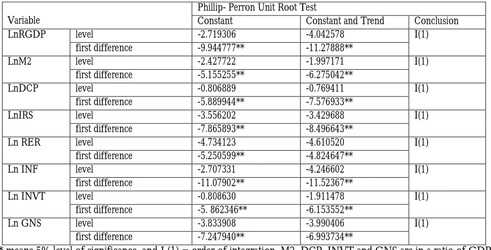
Table 4: Result of the Phillip- Perron Unit Root Test
Variable
Phillip- Perron Unit Root Test
Constant Constant and Trend Conclusion
LnRGDP level -2.719306 -4.042578 I(1)
first difference -9.944777** -11.27888**
LnM2 level -2.427722 -1.997171 I(1)
first difference -5.155255** -6.275042**
LnDCP level -0.806889 -0.769411 I(1)
first difference -5.889944** -7.576933**
LnIRS level -3.556202 -3.429688 I(1)
first difference -7.865893** -8.496643**
Ln RER level -4.734123 -4.610520 I(1)
first difference -5.250599** -4.824647**
Ln INF level -2.707331 -4.246602 I(1)
first difference -11.07902** -11.52367**
Ln INVT level -0.808630 -1.911478 I(1)
first difference -5. 862346** -6.153552**
Ln GNS level -3.833908 -3.990406 I(1)
first difference -7.247940** -6.993734**
The Phillip-Perron test in table 4, above also confirms the existence of unit root at first differencing. However, the result of the constant and constant with trend changes, which symbolizes that the time trend is significance. Hence, it is prudent to include it in the regression model of the ADF and PP tests. The graphs of the series as shown in appendix clearly indicate that the series are non stationary in levels, but stationary at first difference.
Table 5: Result of the (CRADF) Test.
Null Hypothesis: E has a unit root Exogenous: Constant
Lag Length: 0 (Automatic - based on SIC, maxlag=1)
t-Statistic Prob.* Augmented Dickey-Fuller test statistic -6.062563 0.0000 Test critical values: 1% level -3.737853
5% level -2.991878
10% level -2.635542
*MacKinnon (1996) one-sided p-values.
The test-statistic on E (-1) is -6.062563, with 24 included observations after adjustment and at 0.05 Mackinnon (1991) critical values is -3.6583. The calculated value of the test statistic is less-than the critical value rejecting the null hypothesis of no co-integration; the series are co-integrated. The presence of co-integration implies that long run equilibrium relationship exists between the dependent variables and the explanatory variables.
Table 6: Result of the Error Correction Model (ECM)
Dependent Variable: DLnRGDP
Variable Coefficient Std. Error t-Statistic Prob
C -0.119738 0.357067 -0.335338 0.7460
DlnM2 0.039200 0.014572 2.690173 0.0360**
DlnDCP 0.671114 0.250445 2.679681 0.0366**
DlnIRS -0.012202 0.003939 -3.097661 0.0101**
DlnRER -2.224718 3.923546 -0.567017 0.5863
DlnINF -1.293295 0.680321 -1.901009 0.0938***
DlnINVT 0.958437 0.490870 1.952526 0.0666***
DlnGNS 0.359798 0.195400 1.841340 0.0821***
DlnRGDP(-1) -0.008892 0.003265 -2.723624 0.0157
DlnM2(-1) 0.352112 0.176747 1.992183 0.0595***
DlnDCP(-1) 0.026781 0.012557 2.132816 0.0443**
DlnIRS(-1) -0.703419 0.137058 -5.132278 0.0001*
DlnRER(-1) -0.667186 1.553625 -0.429438 0.6730
DlnINF(-1) -0.852227 0.235661 -3.616321 0.0021*
DlnINVT(-1) 0.354647 0.159850 2.218624 0.0683***
DlnGNS(-1) 0.324729 0.222193 1.461417 0.1621
E(-1) -0.822830 0.212583 -3.870638 0.0008*
*; ** and *** denote 1 %; 5% and 10% significance level respectively. M2, DCP, INVT and GNS are in a ratio of GDP. R-squared= 0.864970; Adjusted R-squared= 0.611790 DW: 1.982407; Prob (F-statistic) = 0.042375
Other things being equal, after adjustment for the degrees of freedom, the result suggest that about 86.4% of the variation in RGDP is explained by variation in the independent variables. The coefficient of the error correction term E (-1) is -0.822830 as measure of the speed of adjustment which is negative and statistically significance, it means that during periods of negative shocks and disequilibrium errors to the system, the variables increases less rapidly than consistent and thus moving their lagged values below the long run steady-state path. Due to the negative of the coefficient of the EC term, the total effect is to bring back the changes of variables to their long run trajectory as determined by the system. This implies that for any drift away from the long run equilibrium in previous years, convergence to the equilibrium is corrected by 82.2%. That is approximately 82.2% of the error is corrected every year in the event of shocks in the system
Table7: Result of the Granger Causality Tests
Hypothesis No. of lags F-Stat Prob. Conclusion
DLnM2 does not Granger Cause DLnRGDP DLnRGDP does not Granger Cause DLnM2
2 5.35561 0.0201** Bi-directional
Relationship
2 4.68222 0.0277**
DLnDCP does not Granger Cause DLNRGDP DLnRGDP does not Granger Cause DLnDCP
2 2
4.54653 0.0252** Uni directional
Relationship
1.56223 0.2368
DLnIRS does not Granger Cause DLnRGDP DLnRGDP does not Granger Cause DLnIRS
2 1.47241 0.2557 Unidirectional
Relationship
2 6.26304 0.0086*
DLnRER does not Granger Cause DLnRGDP DLnRGDP does not Granger Cause DLnRER
2 11.6602 0.0012* Bi-directional
Relationship
2 3.17357 0.0730***
DLnINF does not Granger Cause DLnRGDP DLnRGDP does not Granger Cause DLnINF
2 2.52536 0.1080 Unidirectional
Relationship
2 3.35345 0.0578**
DLnINVT does not Granger Cause DLnRGDP DLnRGDP does not Granger Cause DLnINVT
2 3.98852 0.0368** Unidirectional
Relationship
2 0.12520 0.8831
DLnGNS does not Granger Cause DLnRGDP DLnRGDP does not Granger Cause DLnGNS
2 0.34942 0.7098 Unidirectional
Relationship
2 0.34942 0.0704***
*, ** and *** indicates that the null hypothesis is rejected at 1%, 5% and 10% level of significance respectively. The appropriate lag length is selected based on the Schwarz Information Criteria (SIC), the test is performed on the stationary data series. M2, DCP, INVT and GNS are in a ratio of GDP
The result of the Granger causality test in table 7, above indicates a bi-directional relationship between M2 and RDGP at 5% respectively. DCP granger causes RGDP at 5%, RGDP granger causes IRS at 1%. RER and RDGP exhibit a bi-directional relationship at the level of their p-values. There exist a unidirectional relationship between INF and RGDP; the causation runs from RGDP to INF at 5% level of significance. Causation runs from INVT to RGDP at the 5% level of significance and does not run in the reverse sense. RGDP granger causes GNS at the level of their p-values. In general, the Granger causality test result demonstrates a fairly strong evidence of a casual relationship between financial development and the growth of output. Hence, confirming the hypotheses that causality exists between financial development and economic growth in Sierra Leone. This could also be seen from the series that there is a strong speed of adjustment as it can correct about 82.2 % convergence to equilibrium following a shock to the system.
5. Conclusion
This result is consistent with the study by Mckinnon (1973), Shaw (1973) and Patrick (1966) that causation of finance and growth could be bi-directional or unidirectional (Supply-leading or demand leading impetus). Our findings also reveal that domestic credit to the private sector has a positive effect on the growth of output; this implies that an increase in the domestic credit to the private sector encourages private investment and hence increases growth. High interest rate margin as observed in the study impacts negatively on growth. This signals that the banking sector in Sierra Leone is relatively uncompetitive. With an uncompetitive banking sector, the cost of capital is very high and therefore slowing down investment and growth. Therefore, competitive interest rate spread and compliance with financial institutions legal instruments to make the financial sector more responsive to the needs of the Sierra Leone populace should be encouraged
Inflation and exchange rate are found to negatively impact on the growth of output. Therefore, to create the enabling environment for investments, the exchange rate should be stabilized and low inflation rate maintained. Since low inflation rates is likely to bring high real interest rates, which may positively affect private investment and hence growth. Hence, the Government should strive to attain sound macroeconomic climate, loan administration capacity and a more efficient financial system. This is because; a more efficient financial system could positively impact on economic growth and hence increasing employment and growth. Since, economic growth is conventionally expected to reduce poverty
Despite data limitation, our findings have an important implication not only for policy makers in Sierra Leone but also for development organizations that are assisting in the growth process of Sierra Leone and other Africa countries. On this basis, we look forward to future study on growth issues with a view to further provoke policy discourse, such study could be the nexus between Bank risks management and Bank performance in Sub-Saharan Africa countries.
References
Arestis, P. and Demetriades, P. (2001), “Financial Development and Economic Growth: Assessing the Evidence”,
Economic Journal, 107: 783-799.
Athukorala, P. (1998), “Interest Rates, Saving and Investment”: Evidence from India, Oxford Development Studies, 26 (2)
pp.153-169.
Barro , R . J. (1989a), “A Cross Country Study of growth, saving and Government.” National Bureau of Economic
Research Working Paper No. 2955, February.
Bencivenga V.R and Smith, B. D. (1977) “Financial Intermediation and Economic Growth in Least Developed Countries” A Theoretical Approach, Journal of Development Studies Vol .6 No.3), pp. 58-72
Bencivenga,V.R. and Smith, B.D. (1991) “Financial Intermediation and Endogenous Growth.” Review of Economic
Studies, Vol .58 (April), pp. 195-209.
Beck, T.A. Demirgüç-Kunt, and V. Maksimovic (2008), “Financial and Legal Constraints to Firm Growth: Does Size Matter?” Journal of Finance,
Bank of Sierra Leone Annual Report (2011), pp.37 http:// www.bsl.gov/pdf (Accessed 15 November, 2012)
Diamond, D. and Dybvig, P. (1983), “Bank Runs, Deposit Insurance, and Liquidity”, Journal of Political Economy, 85, p.
191-206.
Dickey, D A and Fuller, W.A. (1979) ‘Distribution of the estimators of autoregressive time series with a unit root,’
Journal of the American Statistical Association, Vol.74, No. 2, pp. 427-31
Dornbusch, R. and Reynoso, A. (1989), “Financial Factors in Economic Development”, American Economic Review,
Papers and Proceedings 79: pp. 204-9.
Demirgüç-Kunt, A. and Maksimovic, V. (2005) “Stock Markets Development and financing Choices of Firms”, World
Bank Economic Review,10 (2): pp. 341-70.
Engel, R F and Granger, C.W.J (1987) ‘Co-integration and error correction: Representation estimation and testing’, Journal
of Econometrica, Vol. 55, No.3, pp. 251-76
Flamimi, C. Valentina C. McDonald, G. and Liliana, S. (2009), “The Determinants of Commercial Banks Profitability in Sub-Saharan Africa” IMF Working Paper.
Financial Sector Development Plan Report for Sierra Leone (2009), pp 23-45.
Granger, C.W. J. (1969) ‘Investigating causal relations by econometric models and cross-spectral Methods’
Econometrica, Vol. 37, No.2, pp 13-15
Gelbard , E. and Pereira Leite , S. (1999) “Measuring Financial Development in Sub- Saharan Africa”, IMF Working
Paper 99/105, Washington DC: International Monetary Fund.
Hendry, D F and Richard, W. R. (1983) ‘Econometrics-alchemy or science,’ Journal of Economic, Vol. 47, No. 13, pp.387-406
Hannan, E.J and B.G Quinn (1979) Determination of the Order of an Autoregression‟, Journal of the Royal Statistical
Society, Series B, 41, 190-195
International Financial Statistics Data Base (2011) http://www.ifs.org (Accessed 16 April, 2012)
Lanyi, A . and Saracoglu, R.(1989) “Interest rate policies in developing countries.” Occasional Papers 22, International
Monetary Fund (October, 1989).
Mackinnon, J G (1991). Critical values for co-integration tests‟, in RF Engle and CWJ Granger (eds) Long-run Economic
Relationships Oxford: Oxford University Press pp.267-76
Mattesini, F. (1996), “Interest Rate Spreads and Endogenous Growth”. Economic Notes; V.25-No.1, pp. 111-129. McKinnon, R.I.(1973) Money and Capital in Economic Development. Washington, D.C: Brookings Institution.
Odedokun ,M. O. (1996), “Alternative Econometric Approaches for Analyzing the Role of Financial Sector in Economic Growth: Time Series Evidence from LDCs.”
Patrick, H.(1966),“Financial Development and Economic Growth in Under-developed Countries.” Economic
Development and Cultural Change, 14(2): pp. 174 – 89.
Pagano, M. (1993) “Financial Markets and Growth: An Overview”, European Economic Review, 37 (2-3) pp. 613-22. Phillips, P C B and Perron, P. (1988)’ Testing for unit root in times series regression,’ Journal of Biometrica, Vol. 75, No.
6, pp.335-46
Quantitative Micro Software (2007). EViews 6 User‟s Guide, Irvine: Quantitative Micro Soft Ware
Romer, P.M. (1986) “Increasing Returns and Long run Growth.” Journal of Political Economy, Vol. 94, No.4, pp. 1002 – 37.
Schumpeter, Joseph A. (1969), The Theory Of Economic Development (Oxford: Oxford University Press) Shaw, E.S.(1973) Financial Deepening in Economic Development. New York: Oxford University Press.
Stiglitz , J.E.(1993) Overview, in Finance and Development: Issues and Experience, (Ed) Giovanini (Cambridge University Press, Cambridge) , pp. 343-53.
Soyibo, A. (1997) “Financial Liberalization and Bank Restructuring in Sub-Sahara Africa : Some Lessons for Sequencing and Policy Design’’. Journal of African Economies, Vol 6 (1) pp. 100- 150.
Sierra Leone Agenda for Change (2008) http:// www.mofed.sl.gov/pdf (Accessed 15 November, 2008)
Warman, F. and Thirlwall , A.P. (1994). “Interest Rates, Saving, Investment and Growth in Mexico 1960-90: Tests of the Financial Liberalization Hypothesis”. The Journal of Development Studies; .30(3): pp.629-647.
World Bank (1994) Adjustment in Africa: Reforms, Results and the Road Ahead, World Bank Policy Research Report, Washington DC: World Bank.
Appendices
Appendix A: Graphs of Level (Non- Stationary)
Appendix B: Graphs of first difference (Stationary)
- 5 - 4 - 3 - 2 - 1 0 1 2 3
8 6 8 8 9 0 9 2 9 4 9 6 9 8 0 0 0 2 0 4 0 6 0 8 1 0
L N R G D P
2 . 2 2 . 4 2 . 6 2 . 8 3 . 0 3 . 2 3 . 4
8 6 8 8 9 0 9 2 9 4 9 6 9 8 0 0 0 2 0 4 0 6 0 8 1 0
L N M 2
0.4 0.8 1.2 1.6 2.0 2.4
86 88 90 92 94 96 98 00 02 04 06 08 10
LNDCP 0.8 1.2 1.6 2.0 2.4 2.8 3.2
86 88 90 92 94 96 98 00 02 04 06 08 10
LNIRS 4.4 4.8 5.2 5.6 6.0 6.4
86 88 90 92 94 96 98 00 02 04 06 08 10
LNRER 1.0 1.5 2.0 2.5 3.0 3.5 4.0 4.5 5.0
86 88 90 92 94 96 98 00 02 04 06 08 10
LNINF 0.5 1.0 1.5 2.0 2.5 3.0 3.5
86 88 90 92 94 96 98 00 02 04 06 08 10
LNINV -1.5 -1.0 -0.5 0.0 0.5 1.0 1.5 2.0 2.5
86 88 90 92 94 96 98 00 02 04 06 08 10 LNGNS - 4 - 3 - 2 - 1 0 1 2 3 4
8 6 8 8 9 0 9 2 9 4 9 6 9 8 0 0 0 2 0 4 0 6 0 8 1 0
D L N R G D P
-.6 -.4 -.2 .0 .2 .4 .6
86 88 90 92 94 96 98 00 02 04 06 08 10
-.6 -.4 -.2 .0 .2 .4 .6
86 88 90 92 94 96 98 00 02 04 06 08 10
DLNDCP
-0.8 -0.4 0.0 0.4 0.8 1.2 1.6 2.0
86 88 90 92 94 96 98 00 02 04 06 08 10
DLNIRS
-.8 -.6 -.4 -.2 .0 .2
86 88 90 92 94 96 98 00 02 04 06 08 10
DLNRER
-3 -2 -1 0 1 2 3
86 88 90 92 94 96 98 00 02 04 06 08 10
DLNINF
-0.8 -0.4 0.0 0.4 0.8 1.2 1.6
86 88 90 92 94 96 98 00 02 04 06 08 10
DLNINVT
-3 -2 -1 0 1 2 3 4
86 88 90 92 94 96 98 00 02 04 06 08 10