COOPERATIVE TWO-STAGE NETWORK DEA: A GOAL PROGRAMMING APPROACH

(1)

P. ZAHIRI1, M. MIRBOLOUKI1, §

Abstract. In this study, we present a two-stage data envelopment analysis method dealing with efficiency evaluation of decision making units with network structure. The key point of the study is that the suggested model optimizes the Black-Box and stages efficiencies simultaneously with the aim of achieving the smallest possible gap between the aspiration levels.

Keywords: Data envelopment analysis, two-stage efficiency, multi-objective model, goal programming.

AMS Subject Classification: 90BXX, 90B15, 90CXX, 90C15.

1. Introduction

The main part of the paper begins here. Data envelopment analysis (DEA), developed by Charnes et al. (1978), is a mathematical programming approach for analyzing the relative efficiency of peer decision making units (DMUs) that use multiple inputs to pro-duce multiple outputs. Conventional DEA models treated production units only as Black Boxes with no consideration of the internal processes. Whereas, in the real world, by opening the under evaluated DMUs, they may in fact consist of internal units referred to as sub-units. Network DEA is one important branch of DEA that has been an attractive topic in literature. Most network DEA studies have focused on the two-stage structure in which two stages are connected in series. Indeed, the results obtained through two-stage DEA can be extended to more complex cases. Fre (1991) probably for the first time con-sidered the role of sub-units as an effective factor in efficiency measures. Early studies of two-stage networks treated each stage as a DMU and calculated two stage efficiencies independently and separately; e.g. see Seiford and Zhu (1998) and Wang et al. (1997). Kao (2014) expanded DEA networks in the multi-levels model using the series system.. In all of these models, the weight for intermediate values is assumed to be the same, even it is not important to consider the intermediate values as the output of stage 1 or the input of stage 2.

1

Yadegar-e-Imam Khomeini (RAH) Shahre Rey Branch, Islamic Azad University, Tehran, Iran. e-mail: [email protected]; ORCID: https://orcid.org/0000-0002-2223-3644.

e-mail: [email protected]; ORCID: https://orcid.org/ 0000-0003-1054-8208.

§ Manuscript received: May 2, 2018; accepted: January 5, 2019.

(2)

In two-stage DEA literature, the decomposition approaches, apart from the definition of the stage efficiencies, premise the definition of the overall efficiency of the DMU with a model to decompose the overall efficiency to stage efficiencies. The two basic decompo-sition methods are the multiplicative method of Kao and Hwang (2008) and the additive method proposed by Chen et al. (2009). However, the shortcoming of these decomposition methods is that the overall efficiency to the stage efficiencies is biased and not unique. To overcome the shortcomings of additive and the multiplicative decomposition methods, Kao et al. (2014) introduced an algorithm based on multi-objective programming. Their method includes solving several mathematical programs in order to assess the indepen-dent efficiency score of each stage. Li et al. (2012) introduced a two stage structure by assuming that the inputs to the second stage include both the outputs from the first stage and additional inputs to the second stage. Guo et al. (2016) studied additive effi-ciency decomposition with varying weights and the impact of weight variation on overall efficiency.

Despotis et al. (2015), based on the decomposition paradigm for the structure intro-duced by Li et al. (2012), presented a multi-objective programming approach, capable of dealing with general two-stage processes. Subsequently, Despotis et al. (2016) added a second phase to the last model to identify a Pareto optimal solution. It is notewor-thy to say that both of these methods are nonlinear programming. Based on two last works, Despotis et al. (2016) introduced a linear programming model dealing with com-mon weights of intermediate measures that unlike previous works do not consider external inputs in the second stage.

In this paper, a two-stage process with additional inputs to the second stage as a special kind of network (introduced by Li et al. (2012)) is considered and a new two-stage network DEA method for assessing the peer-efficiency of stage 1 and stage 2 in DEA using multi-objective programming (MOP) is proposed. To solve the suggested MOP model, a goal programming (GP) method as mentioned by Liu and Peng (2008) is used. According to the GP method, the decision maker is asked to set aspiration levels for each objective function. Following this, deviations from these aspiration levels are minimized as an optimal solution.

The remainder of this paper is structured as follows: Section 2 describes, briefly, some network DEA models. In Section 3, our proposed approach is explained. An application of electricity distribution companies of Iran and computational results are provided to illustrate our purposes in Section 4. Finally, in Section 5, concluding comments are made and future extensions are summarized.

2. Preliminaries

This section reviews two preliminary models dealing with efficiency assessments in two-stage processes.

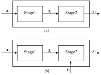
Consider nDMUs, DMUj (j= 1, . . . , n), to be evaluated. Fig 1 illustrates two specific

types of two-stage network structures.

Supposes DMUj transforms m external inputs xj = (x1j, . . . , xmj) to s final outputs

y_j = (y1j, . . . , ysj) via D intermediate measures zj = (z1j, . . . , zDj). For DMUj, xj and zj are inputs and outputs related to the first stage, respectively. Then, zj becomes the input vector of the second stage andy_j is the second stage’s output vector. The network structure depicted in Fig 1.b, as one of the common structures in DEA network literature, allows the second stage to consumeLinputslj = (l1j, . . . , lLj) from outside in addition to

the intermediate measureszj. In this case, according to the basic definition of efficiency,

(3)

calculated as their weighted outputs over their weighted inputs, ase1_o=ψzo

ηxo ande

2

o=

ωyo

ϕzo+µlo

, respectively,

whereη,ψ, ωandµare the vectors of weights associated with the measuresx, z, yandl, respectively. Then, one can evaluate the overall efficiency of the DMUo through the

additive aggregation eoverall_o = (e

1 o+e2o)

2 or the multiplicative aggregation eoverallo = e1o.e2o

of the stage efficiencies. The independent relative efficiency of stage 1 and stage 2, E_o1

Figure 1. Two types of network structure, (a) Two-stage structure of DMUj,

(b)Two-stage structure of DMUj with additional inputs to the second stage.

and E_o2, under constant returns to scale (CRS), can be obtained by solving the following conventional DEA models that was introduced by Charnes et al. (1978) and named the CCR model, respectively:

E_o1=max

PD d=1ψdzdo Pm

i=1ηixio

s.t.

PD d=1ψdzdj Pm

i=1ηixij≤1 ∀j

ψd, ηi≥0 ∀d, i

(1)

E_o2= max

Ps r=1ωryro PD

d=1ψdzdo+PLk=1µklko

s.t.

Ps r=1ωryrj PD

d=1ψdzdj+PLk=1µklkj

≤1 ∀j

ψd, µk, ωr≥0 ∀d, k, r

(2)

(4)

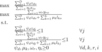
extended the centralized method introduced by Liang et al. (2008) for the structure in Fig 1.b. They proposed a heuristic approach based on a parametric linear programing model. Despotis et al. (2015) considered a multi-objective programming framework to evaluate the cooperative efficiencies as follows:

max

PD d=1ψdzdo Pm

i=1ηixio

max

Ps r=1ωryro PD

s.t.

PD d=1ψdzdj Pm

i=1ηixij≤1 ∀j Ps

r=1ωryrj PD

≤1 ∀j

ψd, µk, ωr, ηi≥0 ∀d, k, r, i

(3)

As inspection makes clear, the vector (E1_o, E_o2) is the ideal point in the objective functions space of the multi-objective model (3). The authors employed theL∞ norm to locate the

stage efficiencies as close as possible to their ideal values, by minimizing the maximum of the deviations (E_o1 −e1_o) and (E_o2 −e2_o) from the ideal point E_o1, E_o2

. Accordingly, Despotis et al. (2015) proposed the following model (Despotis model hereafter):

min δ s.t.

PD

d=1ψdzdo+δ≥Eo1

E2

o−δ

PD

−Ps

r=1ωryro≤0

Pm

i=1ηixio= 1

PD

d=1ψdzdj−Pim=1ηixij≤0 ∀j

Ps

r=1ωryrj−

PD

d=1ψdzdj−

PL

k=1µklkj≤0 ∀j

ψd, µk, ωr, ηi≥0 ∀d, k, r, i

(4)

where δ denotes the largest deviation. Suppose (ψ∗,ω∗,η∗,µ∗,δ∗) ∈ RD+s+m+L+1 is the

optimal solution of model (4), then the efficiency scores for DMUo in the first and the

second stage along with overall efficiency are calculated as follows:

e1_Des.,o=ψ

∗_z

o

η∗xo, e 2

Des.,o=

ω∗y_o ψ∗zo+µ∗lo

, eOverall_Des.,o =e1_Des.,o.e2_Des.,o

However, model (4) is non-linear and, as it will be illustrated later in section 4, in spite of the notable idea of cooperating state of assessing efficiencies of stages in Despotis model, the results are close to the independent and there is in actuality no cooperative response. In the next section, model (3) applying a GP approach is linearized at first and then an extension of it as a three-objective model is considered.

3. The proposed cooperative two-stage efficiencies

(5)

3.1. Developing the proposed model in a Two-objective programming. Inspired by the procedure used in Liu and Peng (2008) and applying GP method, model (3) can be converted to the following model:

min α−+α+ min β−+β+

s.t.

PD d=1ψdzdo Pm

i=1ηixio +α

−_−α+₌_A ₍₅_a₎

PD d=1ψdzdj Pm

i=1ηixij ≤1 ∀j (5b)

Ps r=1ωryro PD

d=1ψdzdo+PLk=1µklko+β

−_−β+₌_B ₍₅_c₎

Ps r=1ωryrj PD

≤1 ∀j (5d)

ψd, µk, ωr, ηi ≥ε ∀d, k, r, i

α−, α+, β−, β+≥0

(5)

where A and B are the aspiration levels and ε > 0 is a non-Archimedean infinitesimal value. α−, α+, β− and β+ are goal deviations. According to the definition of relative efficiency, each DMU desires to approach an unity value as the scoring efficiency (i.e. A = B = 1). Consequently, α+ and β+ as the over-achievement of goals cannot take the positive value and can be omitted. To reach the smallest gap between the aspiration levels (unity value of the efficiency score) the fractions in constraints (5a) and (5c) must be increased by increasing the numerator and/or decreasing the denominator, through adding α+ and β+ to the numerator and taking α− and β− away from denominator of these fractions, respectively. Regarding these considerations, model (5) can be written as:

min α−+α+ min β−+β+

s.t.

PD

d=1ψdzdo+α+ Pm

i=1ηixio−α−= 1 (6a)

PD

d=1ψdzdj−

Pm

i=1ηixij≤0 ∀j

Ps

r=1ωryro+β +

PD

d=1ψdzdo+PLk=1µklko−β

−= 1 (6b)

Ps

r=1ωryrj−

PD

d=1ψdzdj−

PL

k=1µklkj≤0 ∀j

ψd, µk, ωr, ηi≥ε ∀d, k, r, i

α−, α+, β−, β+≥0

(6)

An easy computation shows that constraints (6a) and (6b) can be rewritten as follows, respectively:

PD

d=1ψdzdo−Pmi=1ηixio+α++α− = 0

Ps

r=1ωryro−

PD

d=1ψdzdo−PLk=1µklko+β

+

(6)

Now, by substitutionα++α− andβ++β− withαandβ, respectively, and according to the Min-Max formulation, model (6) can be simplified to the following linear model:

min δ

s.t.

PD

d=1ψdzdo−

Pm

i=1ηixio+α = 0

PD

d=1ψdzdj−Pim=1ηixij≤0 ∀j

Ps

r=1ωryro−

PD

d=1ψdzdo−

PL

k=1µklko+β= 0

Ps

r=1ωryrj−PDd=1ψdzdj−PLk=1µklkj≤0 ∀j

0≤α≤δ 0≤β≤δ

(7)

Theorem 3.1. Model (7) is a feasible model.

Proof. Let ψ_d =ε; ∀ d∈ {1, . . . , D}, ωr =ε; ∀ r ∈ {1, . . . , s}, ηi =M; ∀ i∈ {1, . . . , m}

and µ_k = M; ∀ k ∈ {1, . . . , L}, where M is a big positive number that can be chosen

by M > max{max

j {

εPD_d=1zdj Pm

i=1xij }, max_j {

ε(Pm_r=1yrj−PDd=1zdj) PL

k=1lkj

}}. Now let α = MPm

i=1xio − εPD

d=1zdo, β = M

PL

k=1lko−ε(

Pm

r=1yro −

PD

d=1zdo) and δ = max{α, β}. It can be easily seen that (ψ,ω,η,µ, α, β, δ) is a feasible solution for model (7).

Suppose that model (7) is solved and the optimal solution (ψ∗, ω∗, η∗, µ∗, α∗, β∗, δ∗)∈

RD+s+m+L+3is at hand. Now, considering the constrains of model (7) and the definitions

of the efficiencies of the first and second stages as e1_o=ψ zo

η xo and e

2

o =

ω yo

ψ zo+µ lo , we

have

ψ∗zo+α∗=η∗xo ⇒ α∗ =η∗xo 1−e1o

ω∗y_o+β∗ =ψ∗zo+µ∗lo ⇒ β∗ = (ψ∗zo+µ∗lo)(1−e2o)

As a result, through solving model (7), the efficiency score of DMUo in stage 1 and stage 2 can be calculated as follows, respectively:

e1_o = (1− α

∗

η∗xo

) , e2_o∗= (1− β

∗

ψ∗zo+µ∗lo

)

Consequently, the overall efficiency is defined as the product of individual efficiencies of the two stages (eOverall

o =e1o .e2o ).

Definition 3.1.DMUo is non-dominated if and only ifα∗+β∗ = 0in the optimal solution

of model (7).

(7)

basic model for DMUo: max

hPD d=1ψdzdo Pm

i=1ηixio ,

Ps r=1ωryro PD

d=1ψdzdo+PLk=1µklko,

Ps r=1ωryro Pm

i=1ηixio+PLk=1µklko i

s.t.

PD d=1ψdzdj Pm

i=1ηixij≤1 ∀j

Ps r=1ωryrj PD

≤1 ∀j

Ps r=1ωryrj Pm

i=1ηixij+PLk=1µklkj

≤1 ∀j

(8)

Theorem 3.2. Model (8) is a feasible model.

Proof. Let ψ_d = ε; ∀ d∈ {1, . . . , D}, ωr = ε;∀ r ∈ {1, . . . , s},ηi =M;∀ i ∈ {1, . . . , m}

andµ_k=M;∀k∈ {1, . . . , L}. Where εand M are infinitestimal and big positive values, respectively. (ψ,ω,η, µ) is a feasible solution for model (8).

Carrying out the same process used in the previous section and introducing the new variablesα, β and ρ, model (8) can be represented as the following linear programming:

min δ s.t.

PD

d=1ψdzdo−

Pm

i=1ηixio+α = 0 (9a)

PD

d=1ψdzdj−Pmi=1ηixij≤0 ∀j (9b)

Ps

r=1ωryro−

PD

d=1ψdzdo−

PL

k=1µklko+β= 0 (9c)

Ps

r=1ωryrj−PDd=1ψdzdj−PLk=1µklkj≤0 ∀j (9d)

Ps

r=1ωryro−

Pm

i=1ηixio−

PL

k=1µklko+ρ= 0 (9e)

Ps

r=1ωryrj−Pmi=1ηixij−PLk=1µklkj≤0 ∀j (9f)

0≤α≤δ (9g)

0≤β≤δ (9h)

0≤ρ≤δ (9i)

(9)

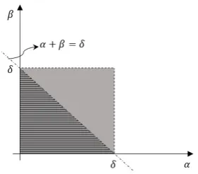
Note that the set of constraint (9f) is redundant due to constraints (9b) and (9d). Also, constraints (9a) and (9c) result ρ = α + β that by which it can be concluded that constraints (9g) and (9h) are redundant. Then model (9) is summarized as the following model:

min δ s.t.

PD

d=1ψdzdo−Pim=1ηixio+α = 0

PD

d=1ψdzdj−

Pm

i=1ηixij≤0 ∀j

Ps

r=1ωryro−PDd=1ψdzdo−PLk=1µklko+β= 0

Ps

r=1ωryrj−

PD

d=1ψdzdj−

PL

k=1µklkj≤0 ∀j

α+ β ≤δ

α, β≥0

(10)

(8)

Figure 2. Image of feasible regions of model (7) and (10) in the space of variables αandβ.

optimal solution of model (10), the efficiency score of each stage, Black Box and overall are calculated through the following equations:

e1_o= (1−_ηα∗∗_x o)

e2_o = (1−_ψ∗_zβ∗ o+µ∗lo)

eBlack_o −Box =1− δ∗

η∗_x o+µ∗lo

eOverall_o =e1_o×e1_o

Definition 3.2. DMUo is non-dominated in model (10), if and only if δ∗ = 0 in the

optimal solution of model (10).

In our proposed method, similar to the Despotis method, a multi-objective mathe-matical program is used in order to simultaneously optimize the efficiencies of sub-units (model (7)), but with the difference that the aspiration levels are considered to be 1. We also formulate another multi-objective model to simultaneously optimize the efficiencies of sub-units along with Black Box efficiency.

Remark 3.1. The Black Box efficiency score eBlack Box_j is obtained directly from the optimal solution of model (10), whereas, the overall efficiency eOverall_j is achieved by mul-tiplyinge1_j by e2_j.

4. An application in electricity industry

Tavanir1 Company as an electricity distribution company was founded in 1992 in Iran. This Company was established to undertake the responsibility for the development of electric power generation, transmission facilities and bulk transaction of electricity with the regional electricity companies and large industries.

This section demonstrates an application of the suggested approach in the previous section in performance assessment of electricity distribution companies in Iran. The data and samples are taken from Tavanir’s database for the year 2013. Sixteen electricity distribution companies were selected as DMUs in our analysis. According to the collected data, the power plant (first stage) considering the expenses and consuming available power, exports the generated electric to transmission network (second stage). Then the network,

1_{Tavanir is responsible for all activities that are associated with electric power including generation,}

(9)

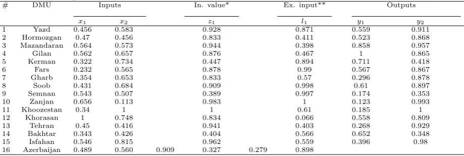
using the imported energy of the system, distributes the electric energy. Table 1 presents the data set. Notice that the data were scaled.

Based upon the data set, five factors related to the performance of electricity distribution companies can be grouped into a two-stage process, as shown in Fig 3 Briefly, the following inputs, intermediate products, and final outputs are considered:

Inputs: Expenses (x₁), Power consumed in the station (x₂), Intermediate products: Electric scale (z₁),

Additional inputs to the second stage: Imported energy (l₁), Outputs: Electric distribution (y1), Electric export (y2).

Figure 3. Electric Distribution Company’s two-stage performance.

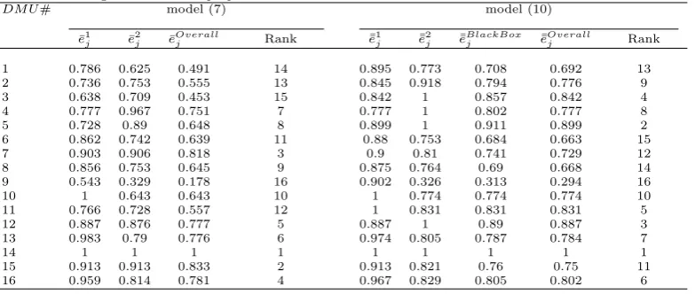
We now apply the mentioned assessment models in the paper to the data set and make the comparison between the proposed method (models (7) and (10)), Despotis model (4) and Independent efficiencies models (models (1) and (2)). Table 2 provides Despotis model and independent efficiencies. The efficiency score of each stage, Black Box and overall calculations via models (7) and (10) are summarized in Table 3. Note here that in Tables 2 and 3 the units are ranked based on overall efficiency.

Table 1. Electric companies data in 2013

# DMU Inputs In. value* Ex. input** Outputs

x1 x2 z1 l1 y1 y2

1 Yazd 0.456 0.583 0.928 0.871 0.559 0.911 2 Hormozgan 0.47 0.456 0.833 0.411 0.523 0.868 3 Mazandaran 0.564 0.573 0.944 0.398 0.858 0.957 4 Gilan 0.562 0.657 0.876 0.467 1 0.865 5 Kerman 0.322 0.734 0.447 0.894 0.711 0.418 6 Fars 0.232 0.565 0.878 0.99 0.567 0.867 7 Gharb 0.354 0.653 0.833 0.57 0.296 0.878 8 Soob 0.431 0.684 0.909 0.998 0.61 0.897 9 Semnan 0.543 0.507 0.389 0.997 0.174 0.353 10 Zanjan 0.656 0.113 0.983 1 0.123 0.993 11 Khoozestan 0.34 1 1 0.61 0.185 1 12 Khorasan 1 0.748 0.834 0.066 0.558 0.809 13 Tehran 0.45 0.416 0.941 0.403 0.268 0.929 14 Bakhtar 0.343 0.426 0.404 0.566 0.652 0.348 15 Isfahan 0.546 0.815 0.962 0.559 0.396 0.98 16 Azerbaijan 0.489 0.560 0.909 0.327 0.279 0.898

* Intermediate value

(10)

Table 2. Despotis and Independent efficiencies results.

DM U# Independent efficiencies Despotis efficiencies

models (1) and (2) model (4)

e1_j e2_j eOverall_j Rank e1_Des.,j e2_Des.,j eOverall_Des.,j Rank

1 0.92 0.943 0.868 14 0.921 0.947 0.872 15 2 0.867 1 0.867 15 0.868 1 0.868 16 3 0.881 1 0.881 11 0.885 1.002 0.887 11 4 0.896 1 0.896 9 0.896 1.009 0.904 9 5 0.927 1 0.927 7 0.936 1.009 0.945 5 6 0.913 0.952 0.87 13 0.917 0.954 0.875 14 7 0.9 1 0.9 8 0.906 1.008 0.913 8 8 0.913 0.954 0.871 12 0.914 0.959 0.877 13 9 1 0.867 0.867 16 1.007 0.87 0.877 12 10 1 0.958 0.958 2 1.006 0.964 0.97 2 11 0.992 0.953 0.945 3 1.001 0.957 0.958 3 12 0.928 1 0.928 6 0.932 1.001 0.934 7 13 0.974 0.958 0.933 5 0.974 0.966 0.941 6

14 1 1 1 1 1 1 1 1

15 0.913 0.972 0.888 10 0.92 0.979 0.901 10 16 0.967 0.97 0.938 4 0.974 0.978 0.952 4

We also include some statistic plots to give a better view of comparisons. Fig 4(I) compares the overall efficiency obtained by independent and Despotis models. As can be seen, the results reveal the similarity of the obtained efficiencies through Despotis with the primary two-stage efficiency assessment models. In other words, Fig 4(I) indicates a small discrepancy graphically between the obtained overall independent and Despotis efficiency. In result, in spite of the notable idea of a cooperating state of assessing efficiencies of stages in Despotis method, the results are so close to the independent and there is no cooperative manner in actuality. This is due to the fact that this method tries to ignore the role of intermediate products in order to fulfill the aspirations; i.e. there is virtually no partnership among sub-units taking place.

Table 3. Resulting Efficiencies for proposed model.

DM U# model (7) model (10)

¯

e1

j e¯2j ¯eOverallj Rank e¯¯1j e¯¯2j ¯¯eBlackBoxj ¯¯eOverallj Rank

1 0.786 0.625 0.491 14 0.895 0.773 0.708 0.692 13 2 0.736 0.753 0.555 13 0.845 0.918 0.794 0.776 9 3 0.638 0.709 0.453 15 0.842 1 0.857 0.842 4 4 0.777 0.967 0.751 7 0.777 1 0.802 0.777 8 5 0.728 0.89 0.648 8 0.899 1 0.911 0.899 2 6 0.862 0.742 0.639 11 0.88 0.753 0.684 0.663 15 7 0.903 0.906 0.818 3 0.9 0.81 0.741 0.729 12 8 0.856 0.753 0.645 9 0.875 0.764 0.69 0.668 14 9 0.543 0.329 0.178 16 0.902 0.326 0.313 0.294 16 10 1 0.643 0.643 10 1 0.774 0.774 0.774 10 11 0.766 0.728 0.557 12 1 0.831 0.831 0.831 5 12 0.887 0.876 0.777 5 0.887 1 0.89 0.887 3 13 0.983 0.79 0.776 6 0.974 0.805 0.787 0.784 7

14 1 1 1 1 1 1 1 1 1

15 0.913 0.913 0.833 2 0.913 0.821 0.76 0.75 11 16 0.959 0.814 0.781 4 0.967 0.829 0.805 0.802 6

(11)

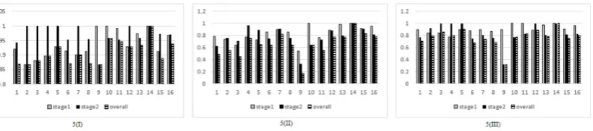
nature of work among sub-units without resulting in improvement in the overall efficiency will result in high rank for this DMU. Returning to the results shown in table 3, there is a kind of cooperation between stages, instead of competition, with the aim of improving the overall efficiency. In other words, comparing Fig 5(I) with Figs 5(II) and 5(III), one can observe a significant increase in the overall efficiency for most DMUs. It should be noted that according to Fig 4(II), there is not much difference between peer-performance Black Box efficiencyeBlack Box_j and overall efficiencyeOverall_j . This shows that model (10) yields peer-performance Black Box efficiency so that we can estimate the overall efficiency without doing the additional operation. It can easily be seen that Figs 5(II) and 5(III) reveal a modification in the efficiency measure of a sub-unit in order to proportionate with the efficiency of another sub-unit by models (7) and (10) in comparison with Fig 5(I).

Consider again DMU3. Looking at the obtained results for this unit in Tables 3, it can be seen that model (7) yields a fair efficiency score for sub-units. However, this appropriate efficiency between two stages leads to this unit having rank 15. While solving model (10) for DMU3 leads to not only the proportionate assessment of efficiencies in stages 1 and 2, it also leads to a better rank for this unit of 4.

It is worth stressing that the obtained results after solving model (10) provide important managerial information for performance analysis and improvement. In fact, the causes of inefficiency and shortcomings of inefficient units are easy to identify when taking a managerial perspective on the distribution of efficiencies (overall and sub-unit efficiency) in Fig (7III). For instance, for the inefficient unit DMU10 (Zanjan) there is a significant difference between the efficiency score of stages 1 and 2. In this case, given that stage 1 is efficient, and stage 2 is inefficient, the expansion of manufacturing capacity in stage 2 could be a management strategy to improve the overall performance. This means preparing further distribution and export companies as the fundamental solution to improve the performance of the company. Furthermore, it means paving the way of distribution and export as the fundamental solution to improve the overall performance of this company. Now if there is an insignificant difference between the efficiency of the sub-units of an inefficient unit, it can be concluded that the cause of inefficiency is due to the Black Box performance of the evaluated company.

Figure 4. 4(I) Comparing the overall efficiency obtained by independent and Despotis models, 4(II) Comparing the results of ¯e¯BlackBox

j and ¯e¯Overallj efficiencies,

Comparing the results of ¯eOverall

j and ¯e¯Overallj efficiencies

5. Conclusion

(12)

Figure 5. Efficiency distribution of stage one, two and overall resulted from independent models (5(I)), model (7) (5(II)), model (10) (5(III)).

to examine the efficiency of DMUs with some stages referred to as sub-units. This paper develops a method based on the MOP model for performance assessment of a specific two-stage network DEA. To this end, we first obtain a linear program by converting a MOP model with the objectives of maximizing both stage efficiencies to a linear program with respect to the GP method. We then extend the obtained model and develop a new model that optimizes the efficiency of each two stages and Black Box efficiency simultaneously. The key point here is that the suggested model optimizes the Black Box and divisional efficiencies with the aim of achieving the smallest possible gap between the aspiration lev-els (unity value of the efficiency score) simultaneously. In result, an important managerial point can be made that applying the suggested model causes a type of cooperation between stages, with the aim of improving the overall efficiency. To illustrate the features and the applicability of the proposed models, the performance of Iranian electricity distribution companies was studied.

References

[1] Charnes, A., Cooper, W. W. and Rhodes, E., (1978), Measuring the efficiency of decision making units, Eur. J. Oper. Res., 2 (6), pp. 429444.

[2] Chen, Y., Cook, W. D., Li, N. and Zhu, J., (2009), Additive efficiency decomposition in two-stage DEA. Eur. J. Oper. Res., 196(3), pp. 11701176.

[3] Despotis, D. K., Koronakos, G. and Sotiros, D. (2015), A Multi-objective Programming Approach to Network DEA with an Application to the Assessment of the Academic Research Activity. Procedia Comput. Sci., 55, 370379.

[4] Despotis, D.K., Koronakos, G. and Sotiros, D. (2016), Composition versus decomposition in two-stage network DEA: a reverse approach. J. Prod. Anal., 45(1), pp. 71-87.

[5] Despotis, D.K., Sotiros, D. and Koronakos, G. (2016), A network DEA approach for series multistage processes, Omega, 61, 35-48.

[6] Fre, R. (1991), Measuring Farrell Efficiency for a Firm with Intermediate Inputs. Academe. Econ. Pap., 19, 329340.

[7] Farrell, M. J. (1957), The Measurement of Productive Efficiency. J. R. Stat. Soc. Ser. A-G, 120(3), pp. 253.

[8] Guo, C., Shureshjani, R.A., Foroughi, A.A. and Zhu, J. (2017), Decomposition weights and overall efficiency in two-stage additive network DEA. Eur. J. Oper. Res., 257, 896-906.

[9] Kao, C. (2014), Efficiency decomposition for general multi-stage systems in data envelopment analysis. Eur. J. Oper. Res., 232(1), pp. 117124.

[10] Kao, C. and Hwang, S.-N. (2008), Efficiency decomposition in two-stage data envelopment analysis: An application to non-life insurance companies in Taiwan. Eur. J. Oper. Res., 185(1), pp. 418429. [11] Kao, H.Y., Chan, C.Y. and Wu, D.-J. (2014), A multi-objective programming method for solving

network DEA. Appl. Soft Comput., 24, 406413.

(13)

[13] Liang, L., Cook, W. D. and Zhu, J. (2008), DEA models for two-stage processes: game approach and efficiency decomposition. Nav. Res. Log., 55, 64353.

[14] Liu, F. H. F. and Hsuan Peng, H. (2008).Ranking of units on the DEA frontier with common weights. Comput. Oper. Res., 35(5), pp. pp. 16241637.

[15] Seiford, L. M. and Zhu, J. (1998), On alternative optimal solutions in the estimation of returns to scale in DEA. Eur. J. Oper. Res., 108(1), pp. pp. 149152.

[16] Wang, C. H., Gopal, R. D. and Zionts, S. (1997), Use of Data Envelopment Analysis in assessing Information Technology impact on firm performance. Ann. Oper. Res., 73(0), pp. pp. 191213. [17] Yu, Y. and Shi, Q. (2014), Two-stage DEA model with additional input in the second stage and part

of intermediate products as final output. Expert Syst. Appl., 41(15), pp. pp. 65706574.

Parisa Zahiriis a Ph.D. candidate at the Department of Mathematics, Yadegar-e-Imam Khomeini (RAH) Shahre Rey Branch, Islamic Azad University, Tehran, Iran. She has worked as a Mathematics teacher for 23 years in high school. Her major research interest includes Operations Research and Data Envelopment Analysis.