R E S E A R C H A R T I C L E
Open Access
Odds ratios from logistic, geometric,
Poisson, and negative binomial regression
models
Christopher J. Sroka
1*and Haikady N. Nagaraja
2Abstract
Background: The odds ratio (OR) is used as an important metric of comparison of two or more groups in many biomedical applications when the data measure the presence or absence of an event or represent the frequency of its occurrence. In the latter case, researchers often dichotomize the count data into binary form and apply the
well-known logistic regression technique to estimate the OR. In the process of dichotomizing the data, however, information is lost about the underlying counts which can reduce the precision of inferences on the OR.
Methods: We propose analyzing the count data directly using regression models with the log odds link function. With this approach, the parameter estimates in the model have the exact same interpretation as in a logistic
regression of the dichotomized data, yielding comparable estimates of the OR. We prove analytically, using the Fisher information matrix, that our approach produces more precise estimates of the OR than logistic regression of the dichotomized data. We also show the gains in precision using simulation studies and real-world datasets. We focus on three related distributions for count data: geometric, Poisson, and negative binomial.
Results: In simulation studies, confidence intervals for the OR were 56–65% as wide (geometric model), 75–79% as wide (Poisson model), and 61–69% as wide (negative binomial model) as the corresponding interval from a logistic regression produced by dichotomizing the data. When we analyzed existing datasets using our approach, we found that confidence intervals for the OR could be up to 64% shorter (36% as wide) compared to if the data had been dichotomized and analyzed using logistic regression.
Conclusions: More precise estimates of the OR can be obtained directly from the count data by using the log odds link function. This analytic approach is easy to implement in software packages that are capable of fitting generalized linear models or of maximizing user-defined likelihood functions.
Keywords: Binary data, Confidence intervals, Count data, Fisher information, Maximum likelihood
Background
Count data arise naturally in many biomedical applica-tions. These data are often converted to binary values and commonly analyzed using logistic regression meth-ods. Usually “failure” for a subject is defined as having a count of zero and “success” as having a positive count. Ifp1 is the probability of a positive count for the group with a risk factor of interest andp2is the probability of a
*Correspondence:[email protected]
1Department of Economics, Applied Statistics, and International Business, New
Mexico State University, MSC 3CQ, PO Box 30001, Las Cruces, NM, 88003-8001 USA
Full list of author information is available at the end of the article
positive count for the group without the risk factor, then the two groups are typically compared using the odds ratio OR=[p1/(1−p1)]/[p2/(1−p2)].
Several examples of this dichotomization approach can be found. From a survey of dietary behaviors among Canadian youth, Vanderlee et al. [1] dichotomized the number of sugar-sweetened beverages consumed and compared the odds of consuming at least one beverage based on gender, age group, and physical activity. A sim-ilar approach was used to estimate the odds of one or more motor vehicle collisions by elderly drivers based on the frequency of falls [2] and the odds of one or more dental caries in children based on diet and obesity [3].
In some applications, the cutpoint of interest for the OR is not always at one. Van Strien et al. [4] defined fre-quent falls to be more than two in the past year, and dichotimized the count data around this value to cal-culate the odds of frequent falls associated with taking psychotropic medications. Duggal et al. [5] fit two sepa-rate models to examine the number of outpatient visits to Veterans Administration (VA) facilities. A logistic regres-sion model was applied to the binary data of use or non-use of the VA facilities and a separate negative bino-mial (NB) model (with support of positive integers) was used for the count data of the frequency of visits among those who had at least one visit.
The loss of information from dichotomizing a contin-uous variable prior to analysis has been studied exten-sively. Suissa and Blais [6] examined dichotomizing con-tinuous variables above and below thresholds of clin-ical interest (e.g., patients with cholesterol higher or lower than 240 mg/dl). They developed an approach for modeling the probability of being above the clini-cal threshold using a generalized linear model (GLM) framework and demonstrated the gains in information using this approach instead of a logistic regression with dichotomized values. Moser and Coombs [7] developed a method to estimate the OR directly from a continu-ous regression model by assuming that the errors follow a logistic distribution. Suissa [8] and Peacock et al. [9] applied the delta method to obtain an estimator and stan-dard error for the OR (as well as other metrics of risk) using the sample mean and standard deviation from a normal distribution.
Research on the loss of information from dichotomiz-ing count data is limited. Recently, Preisser et al. [10] examined the information loss in logistic regression when compared to a special two-part hurdle model with trun-cated Poisson or NB distribution for the observed count data. These models have separate parameters for altering the probability of zero counts and the mean of the trun-cated distribution used for positive counts. It is assumed the two parts of the model are related, with their link func-tions having common regression parameters involving covariates. The critical assumption is given in condition (6) of their paper. It assumes that the logit link func-tion for the zero count and the log mean link funcfunc-tion for the truncated count distribution are linearly related. The crucial difference between their hurdle model and the corresponding ordinary Poisson or NB count models is that their condition (6) is incompatible for these distribu-tions. However it is compatible for the geometric model, in which case the link functions are identical.
Methods
We propose analyzing the non-dichotomized data using count regression models with the log odds link function
and demonstrate this method with the geometric, Pois-son, and NB distributions. These three distributions are related to each other and can be used to model a wide range of overdispersion in the count data. We compare inference for the OR using our method to the logistic regression approach that dichotomizes the count data. Our focus is on analyses that compare the odds of a pos-itive count between two groups (cutpoint at zero). The use of the log odds link function results in model param-eters being compatible with the usual logistic regression model and enables us to directly compare the resulting covariate dependent OR estimates. In addition, the log odds link function is a function of the mean for all of these models and has the real line as the range space. Typically, count regression models use the so-called canonical link function, which differs for the three distributions exam-ined here. As noted by McCullagh and Nelder ([11], p. 32), while the canonical link function has many desirable prop-erties due to its special role in the exponential family of distributions, these properties do not justify its use when the application at hand suggests that a different link func-tion is more appropriate. Here, the desire by researchers to report results in terms of the OR rather than other statis-tics implied by the canonical link (e.g., relative means) supports the use of alternative link functions. Cook ([12], p. 2091) lists some guiding principles on the choice of a link function.
Fisher information in dichotomized count variables
LetY be a random variable (r.v.) from a counting process withp = Pr(Y > 0), 0 < p < 1, and support{0, 1,. . .}. Define the binary r.v.Zto equal 0 ifY = 0 and 1 ifY > 0. The r.v.Zfollows the Bernoulli distribution with mean μ = pand variancev(μ) = p(1−p) = μ(1−μ). Letθ denote the odds of a positive count; that is,
θ = Pr(Y >0) Pr(Y =0) =
Pr(Z=1) Pr(Z=0) =
p
1−p. (1)
Then the FI aboutθinZis
FI(Z;θ)= 1
θ (1+θ)2. (2)
We note thatZis not a sufficient statistic for the data generated byY, and we expectFI(Z;θ)to be strictly less than the correspondingFI(Y;θ). We demonstrate this and quantify the magnitude of information loss for the three count models considered.
the link functionh(μ)= log(θ)= log[p/(1−p)] that is linear in them as follows:
log [θ(xi)]=log
p(xi) 1−p(xi)
=xiβ i=1, 2,. . .,n,
(3)
wherexi =(xi0≡1,xi1,. . .,xik)is the 1×(k+1)vector corresponding to thekcovariates associated with a single subjectiandβ =(β0,β1,. . .,βk)is the(k+1)×1 vector of associated coefficients.
The FI inZabout an arbitraryβjin the regression model is
FI(Z;βj)= n
i=1
FI(Zi;θ) ∂θ
∂βj 2
=
n
i=1
p(xi)[ 1−p(xi)]x2ij. (4)
Using general results on GLMs [11], thej,mthelement of the FI matrix forβis given by
−E
∂2(β) ∂βj∂βm
=
n
i=1
w(xi)xijxim, j,m=1,. . .,k,
(5)
whereis the log likelihood function and the weights are
w(xi)=
1
v(μ(xi))[h(μ(xi))]2
, 1≤i≤n. (6)
For the logistic regression model,v(μ) = μ(1−μ) = 1/h(μ)and consequentlyw(x)=p(x)[ 1−p(x)].
In subsequent sections, we use the following result to compare the asymptotic variance of estimators of β by comparing the values of the weightsw(xi)in the FI matrix.
Result 1. LetICbe the FI matrix forβbased on the count dataYwith w(xi) = wC(i). LetIBbe the FI matrix for β based on the dichotomized count dataZwithw(xi) =
wB(i). Ifw∗(i)=wC(i)−wB(i) >0 for alli=1,. . .,n, then the asymptotic variance of the estimator ofβis strictly less under the count model than under the logistic model.
To prove this result, define X(k+1)×n = (x1,· · ·,xn), a matrix associated with the covariates, and W∗n×n = diag{w∗(1),. . .,w∗(n)}, a diagonal matrix with positive diagonal elements. Then it follows thatI∗ = XW∗Xis positive definite. Being FI matrices,IC andIBare already positive definite. Problem 9 in Rao ([13], p. 56) states that ifM2is a positive definite matrix and(M1−M2)is non-negative definite, thenM−21−M−11 is also non-negative definite. By takingM1 = IC andM2 = IB, it means the
diagonal entries of the difference matrixI−B1−I−C1are all positive. Thus we have proved the result.
The geometric regression model
When the count variableY has a geometric distribution with Pr(Y = 0) = 1−p, its probability mass function (pmf ) is given by
Pr(Y=y)=py(1−p), y=0, 1, 2,. . .. (7)
The meanμand variance functions for this geometric pmf are:
μ= p
1−p, v(μ)= p
(1−p)2 =μ(1+μ). (8) The meanμin (8) is nothing but the odds of a positive count (see (1)). LettingθGdenote the odds from the geo-metric distribution and using (2), it can be easily shown that
FI(Y;θG)= 1
θG(1+θG) =(
1+θG)FI(Z;θG). (9)
AsYis non-degenerate,(1+θG) >1 and there is more information in the count r.v. than in the dichotomized r.v. Z. Thus, the asymptotic relative efficiency (ARE) of the MLE of θG based on a random sample of size n from the geometric distribution when compared to the dichotomized data is(1+θG). (See [14], for a definition of the ARE).
Now consider n independent r.v.’s Y = (Y1,. . .,Yn) from the geometric distribution and the corresponding dichotomized variables Z = (Z1,. . .,Zn). The log link functionh(μ)=log(μ)is commonly used in count mod-els [15]. In the case of the geometric distribution, this link function is identical to log[p/(1−p)], the same link function commonly used for models of the dichotomized data, and the covariates affect the parameters through the exact same relationship as in (3). Note that by choosing h(μ)=log(μ)for the geometric model, we are using a dif-ferent link than the canonical link function log(p)implied by (7). Furthermore, for the geometric model
FI(Y;βj)= n
i=1
θ(xi) [ 1+θ(xi)]
x2ij=
n
i=1
p(xi)x2ij. (10)
LetIC represent the FI matrix forβunder the geomet-ric regression model with weightswC(i) = p(xi). Then
aboutβjthat is lost when the geometric count dataYare transformed into binary dataZ.
The Poisson model with log odds link
We now assume that the count r.v.Y follows the Poisson distribution with mean (and variance)μ:
Pr(Y =y)= e
−μμy
y! , y=0, 1, 2,. . .. (11)
The odds of a positive count based on the Poisson distribution,θP, is
θP= Pr(
Y >0) Pr(Y =0) =e
μ−1. (12)
Hence the FI inYand the FI inZgiven in (2) are related as
FI(Y;θP)=
1
(1+θP)2log(1+θP)
=
eμ−1 μ
FI(Z;θP). (13)
The last expression in (13) shows that the proportional increment in the FI inY, given by ∞i=1μi−1/i!, is substan-tial and increases withμ.
With the log odds link function, thenindependent Pois-son r.v.’s Y = (Y1,. . .,Yn) yield (3) with log[θP(xi)]= log{exp[μ(xi)]−1}. Furthermore, the FI in the Poisson r.v.’sYaboutβjis given by
FI(Y;βj)= n
i=1
θP(xi)xij 2
[1+θP(xi)]2log[ 1+θP(xi)]
=
n
i=1
−p(xi) 2
log[ 1−p(xi)]
x2ij
=
n
i=1
wC(i)x2ij, (14)
wherewC(i)is the weight in the FI matrix for the count data. The difference in weights between the count data and the dichotomized data,wC(i)−wB(i)is
p(xi)
p(xi)
−log[ 1−p(xi)]−
[ 1−p(xi)]
. (15)
It is easily shown that for 0 < p(xi) < 1, the quantity within the braces above in (15) is always strictly positive and equals 0 only whenp(xi) = 0, butFI(Y;β1)is unde-fined at this value. Hence, from Result 1, it follows that the Poisson model with the log odds link function produces more efficient MLEs than the logistic model.
The negative binomial (NB) model
The Poisson model assumes that the variance equals the mean, the geometric allows for overdispersion of the form μ(1+μ), and the NB model provides flexibility to model overdispersion with an additional parameter. WhenY fol-lows the NB distribution with mean parameter μ and dispersion parameterδ,
Pr(Y =y)= (y+δ) (y+1)(δ)
δ δ+μ
δ μ δ+μ
y
(16)
for y = 0, 1, 2,. . .. The variance as a function of μ is v(μ)= μ(1+μδ−1). The NB distribution yields the geo-metric distribution whenδ = 1, and the Poisson model is obtained whenδ → ∞. WhenY has NB distribution, Pr(Y>0)=1−[δ/(δ+μ)]δ, and the corresponding odds θ is given by
θ = Pr(Y >0) Pr(Y =0) =
1+ μ δ
δ
−1, (17)
and the mean as a function ofθisμ=δ[(1+θ)1/δ−1]. The second derivative of the log likelihood for a single observationywith respect toθ is
∂2
∂θ2 = −(1+θ)
−2
y μ−1+
y
μ2(1+θ) 1/δ
(18)
and hence the FI in the count random variable,FI(Y;θ), is
(1+θ)1/δ μ(1+θ)2 =μ1 1+μ
δ
δ+1
−1+μ δ
FI(Z;θ). (19)
It is easy to show that whenδ =1,FI(Y;θ)=FI(Y;θG) (given in (9)) and asδ → ∞,FI(Y;θ) = FI(Y;θP)(given in (13)).
We now show that there is more information aboutθin Y than inZ. From (19), it follows that, witht= μ/δ >0, the ratio of the two FIs can be expressed as
(1+t)δ+1−(1+t) tδ
=1+(δ+1)t+(δ+1)δ (1+t0)δ−1t 2
2! −(1+t) tδ
=1+ t
2(δ+1)(1+t0)
δ−1, (20)
The NB regression model typically uses the log link h(μ) = log(μ)to relate the mean of the data to the set of covariates. As noted before, we propose a regression model with log odds link function:
log
1+μi δ
δ −1
=xiβ, i=1, 2,. . .,n. (21)
The FI in the NB r.v.’sYaboutβjis given by
FI(Y;βj)= n
i=1
(1+θ)1/δ μ(1+θ)2θ
2x2
ij. (22)
Now, the difference in weights between the count data and the dichotomized data,wC(i)−wB(i), is
θ(xi) [1+θ(xi)]2
θ(xi)[1+θ(xi)]1/δ
μ −1
, (23)
which is strictly positive since we have shown above that the quantity inside the braces is always positive. Hence from Result 1, we conclude that the MLEs ofβusing the NB regression of the count data are more efficient than the MLEs using logistic regression of the dichotomized data.
The NB regression with log odds link does not fit con-veniently into the GLM framework that uses iteratively weighted least squares for estimation. The model results in the following mean function
μi=δ
1+exiβ
1/δ −1
, (24)
which is a function of bothβand the dispersion parameter δ, and the coefficient of variation is not constant. How-ever, our proposed NB model can be fit by maximizing the following log likelihood with respect toβandδ:
=
n
i=1
log(yi+δ)−log(yi+1)−log(δ)
+yilog
1+exp(xiβ)1/δ−1
−1+yi δ
log[ 1+exp(xiβ)]. (25)
It is done by solving the first order conditions
∂ ∂βj =
n
i=1
xij
yi
δ1+exp(xiβ)1/δ−δ − 1
×
exp(xiβ) 1+exp(xiβ)
=0, (26)
forj=1, 2,. . .,k, and
∂ ∂δ =
n
i=1
(yi+δ)−(δ)
− yilog[ 1+exp(xiβ)] δ21+exp(x
iβ)
1/δ−δ2
=0, (27)
where(a)is the first derivative of(a). In the simula-tion studies and analyses that follow, we use the method of Nelder and Mead [16] to find MLEs ofβandδas imple-mented in the Roptimfunction. The algorithm returns the Hessian at the maximum, which we use to estimate the standard errors of the model parameters. Starting val-ues for the algorithm can be obtained from the coefficient estimates from the corresponding logistic regression and settingδ(0)=1.
Simulation studies
For each distribution (geometric, Poisson, and negative binomial), we conducted a simulation study to quantify the additional precision that can be gained by using a count regression model with log odds link instead of a logistic regression model with the dichotomized data. Count data were simulated from each distribution accord-ing to the followaccord-ing model:
log(θi)= −0.1+0.6x1i−0.55x2i+0.4x3i+0.25x4i (28)
for i = 1, 2,. . .,n. For the NB model, δ = 0.8. Each covariate x1i,. . .,x4i in the model was a binary categor-ical variable. For each sample size used in the study, we simulated a (n× 5) design matrix consisting of a col-umn of ones and a(n×4)matrix of random draws from a Bernoulli(p = 0.5) distribution. Each simulation was repeated 5000 times for sample sizesn= 50, 75, 100, 250, 500, and 1000. For each covariate, the OR and 95% con-fidence limits were calculated from the count and logistic regression models using standard methods. We compared the two approaches based on the percent bias in the esti-mate (measured as the percentage difference between the average of the 5000 estimates and the true OR value), the average mean squared error (MSE) for the log OR, the rel-ative widths of the confidence intervals (measured as the average ratio of the width of the 95% confidence interval from the count regression to the width of the interval from the logistic regression), and actual coverage of the interval (measured as the percent of simulations where the confi-dence interval contained the true OR value obtained from the model in (28)).
would compare to logistic regression when the count distribution is misspecified.
Analysis of real-world datasets
In addition to simulated data, we analyzed real-world datasets to assess the performance of the log odds regres-sion model of the count data. We selected datasets for which a geometric, Poisson, or NB regression model (using log link) had already been determined to provide the best fit. We fit a regression model using the log odds link to each dataset and compared the estimates and stan-dard errors to a logistic regression of the dichotomized data. We briefly describe each dataset below.
German socio-economic panel
Hilbe ([17], p. 295-297) used the geometric count model to describe the number of physician visits by n = 2227 working women in the German Socio-Economic Panel before and after reforms to the German health system in 1997. Reforms included increases in co-payments and limits on provider reimbursement. The survey gathered data on the number of patient visits in 1996 and 1998. The data set is introduced on page 269 of Hilbe [17]. Hilbe initially fit a NB regression model, and upon iden-tifying that the dispersion parameter δ was nearly one, he used the geometric model. He also compared the goodness-of-fit of the canonical link function log(1 − p) to the log mean (or, equivalently, the log odds) link function and concluded that the latter provided a better fit (p. 297).
Australian health survey
Cameron and Trivedi ([15], p.77-80) fit a Poisson model to the number of doctor visits in the past two weeks reported by 5190 single adult respondents to the 1977-1978 Australian Health Survey. They used the canonical link function (that is, log mean) to model the data. In fit-ting a model using the log odds link function, we removed two covariates (age2and presence of a chronic condition that does not limit activity) that were statistically signif-icant in the log mean model but were not statistically significant in either the log odds model or the logistic regression model of the dichotomized data.
General social survey
Agresti ([18], p. 554-555) fit a NB model to count data from the 1990 General Social Survey. The survey asked 1308 participants how many people he/she knew person-ally that were victims of homicide in the past 12 months. Responses ranged from zero to six. The estimated model included an intercept and a single categorical covariate for race:
log(μˆt)= −2.3832+1.7331xt, (29)
whereμˆtis the estimated mean for a respondent of race categorytandxtis an indicator for that respondent’s race (1 = African-American, 0 = white). From the fitted model, Agresti estimated the ratio of means as exp(1.7331)=5.7. We fit the NB model with log odds link to estimate the OR of knowing at least one homicide victim for African-American versus white respondents. For the dichotomized data we applied the well-known asymptotic standard error for the OR calculated from a 2×2 contin-gency table ([18], p. 70), since our covariate of interest is binary.
Results
Simulation studies
Detailed results from the simulation studies are shown in Additional file1to this article.
The percent bias is smaller for the geometric model than the logistic regression of the dichotomized data, and the percent bias decreases as the sample size increases (Additional file 1: Table S.1). In terms of the total error (bias and variance), the MSE of the log OR for the geo-metric model was 29–44% of the MSE for the logistic regression model (Additional file 1: Table S.2). The rel-ative MSE was lower (geometric model more accurate) for smaller sample sizes than for larger sample sizes. As proven in our analytic results, the geometric model con-sistently produced narrower confidence intervals than the logistic regression of the dichotomized data. Confidence intervals calculated directly from the count data were 56– 65% as wide as the intervals from the dichotomized data. The actual coverage of the intervals from the geometric model were slightly below the nominal level of 95% for smaller sample sizes, but never less than 92.7% (n= 50). For sample sizes of 250 or greater, actual coverage was very close to the nominal level.
Additional file1: Table S.9, indicates that the NB model with log odds link produces slightly more biased estimates than the logistic regression model of the dichotomized data. The difference is larger for smaller sample sizes, but diminishes as the sample size increases. In all cases when n ≥ 75, the percent bias does not differ between the two models by more than 1.1 percentage points. Although the NB model produced slightly more biased estimates in many of the simulation scenarios considered, this bias is offset by the lower variance of the NB estimates. Additional file 1: Table S.10 shows the relative MSE of the log OR estimates. For all sample sizes and all param-eters, the estimates from the NB model have a MSE that is at most half of the MSE of estimates from the logis-tic regression model. As an extreme example, for thex2 covariate with sample sizen = 50, the relative MSE is as low as 37%. Additional file1: Table S.11, shows the relative width of those intervals averaged over the 5000 simula-tions. The intervals estimated from the NB model were, on average, shorter by 31–39% of the intervals estimated from the logistic regression model. Both methods produce confidence intervals with coverage that is very close to the nominal 95% level (Additional file1: Table S.12).
We fit the Poisson regression model with log odds link and the logistic regression model to data that were gen-erated with a NB distribution using dispersion parameter values ofδ = 0.5, 1, 5 and 10. The percent bias is shown in Additional file1: Table S.13. In these simulations, the count model with log odds link produced severely biased estimates for the model parameters when there was sub-stantial overdispersion in the data (δ below 5). In some cases, the bias is so severe that the estimates have a sign that is opposite from the true parameter. In con-trast, the logistic regression approach produced estimates with very low bias regardless of how much dispersion there was in the count data. As δ increases to 10, the data become more Poisson-like and the bias is compara-ble to that from the logistic regression model for small sample sizes.
Analysis of real-world datasets
Geometric
Table 1 shows the OR estimates and confidence inter-vals estimated from both models along with the relative width of the confidence intervals, defined as the width of the interval estimated from the geometric model as a percentage of the width of the interval estimated from the logistic model. The table shows that the width of the interval from the geometric model is between 36% and 64% of the width of the interval from the logistic regression model. It also shows that there can be sub-stantial differences in the inferences. For example, the geometric model indicates that women in the oldest age category (50–60 years) had a significantly higher odds
of at least one physician visit (OR = 1.21; p = 0.009) compared to younger women (age 20–39 years). This rather intuitive result was not found in the logistic regres-sion model (OR = 0.99; p = 0.942) because of the lower point estimate and larger standard error produced by that model.
Although the interpretation of the parameters is the same under both geometric and logistic regression, each model is a different method of estimation for those param-eters. Both approaches produce asymptotically unbiased estimators as they are based on the method of maxi-mum likelihood, but each may be biased for small sam-ple sizes. We compared their small samsam-ple bias over a range of sample sizes using the coefficient estimates from the fitted geometric model, given in Table 1 as the true parameter values. We simulated 1000 samples of different sizes ranging from 50 to 500 and applied each method to to obtain the MLEs of the ORs. We then calculated the percent bias, defined as the differ-ence between the average of the 1000 estimates and the true value as a percent of the true value. The results are shown in Additional file 1: Figure S.1. The geomet-ric model almost always has smaller bias that is close to zero, even when there are fewer than 100 observations. The conclusion is that the geometric model produces sub-stantially more accurate and precise estimators than the logistic model when the counts arise from a geometric distribution.
Poisson
Table 2 shows the parameter estimates and 95% confi-dence intervals for the Australian Health Survey data. It also reports the ratio of the widths of the intervals from the Poisson model and the logistic regression model. For all of the covariates, the Poisson model produces narrower intervals with relative widths that ranged from 68%–90%. The statistical inference differs across the two models in two cases (regarding health insurance coverage sta-tus). In both of these cases, the difference arises because the logistic regression produces substantially higher point estimates than the Poisson regression with log odds link (1.30 versus 1.17 for private insurance, 1.53 versus 1.20 for free government insurance due to old age, disability, or veteran status), resulting in statistical significance with the former and nonsignificance with the latter model. For the free government insurance coefficient, the Poisson model has the largest reduction in variance over the logis-tic regression model (average relative width of 68%), but the large difference in point estimates offsets these gains to produce different statistical inferences.
Negative binomial
Table 1OR estimates and 95% confidence intervals from geometric and logistic regression models of physician visits for the German Socio-Economic Panel data
Geometric Logistic Relative widthe
Covariate Estimate Interval Estimate Interval
Post-reforma 0.87 (0.79, 0.96) 0.82 (0.68, 0.99) 57%
Bad healthb 3.13 (2.71, 3.63) 3.28 (2.24, 4.82) 36%
Education (10.5 - 12 years)c 1.09 (0.95, 1.24) 1.19 (0.94, 1.51) 50%
Education (HS graduate +)c 0.97 (0.84, 1.11) 1.32 (1.03, 1.70) 40%
Age (40 - 49 years)d 1.05 (0.93, 1.19) 0.92 (0.73, 1.16) 62%
Age (50 - 60 years)d 1.21 (1.05, 1.39) 0.99 (0.76, 1.29) 64%
Log household income 1.13 (0.99, 1.30) 1.26 (0.98, 1.62) 48%
Reference category:aPre-reform;bGood health;c7 - 10 years of education;dAge 20–39 yearseGeometric compared to logistic model
African-American versus white respondents. The fitted model yielded the following MLEs:
logθ(ˆ t)= −2.5387+1.3154xt
ˆ
δ=0.2023 ˆ
ORNB=exp(1.3154)=3.726. (30)
An approximate 95% confidence interval for log(OR) is (0.9635, 1.6674), which when exponentiated yields an interval of (2.62, 5.30) for the OR. Thus we conclude that African-American respondents had a higher odds of knowing at least one homicide victim compared to white respondents. Note that there is non-zero covariance between the estimator of the regression coefficients and the estimator of the dispersion parameter, unlike the NB model with log mean link ([15], p.82).
From the dichotomized data, we obtainORˆ B = 4.553 andSE
log
ˆ ORB
= 0.217, that leads us to an approx-imate 95% confidence interval (2.98, 6.96) for the OR. In this situation, our conclusion remains the same even
though the NB model produced a lower estimate than the dichotomized data model (3.7 versus 4.6) and an interval that was only 83% as wide.
Discussion
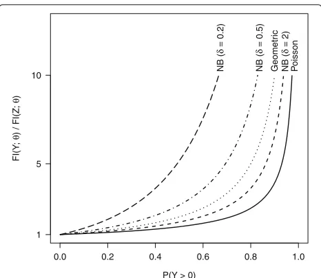
Figure1 shows the relative Fisher informationFI(Y;θ)/ FI(Z;θ) as a function ofp = Pr(Y > 0) for the count models considered in this study. The information lost from dichotomization is modest for small p, but grows exponentially as p → 1. The rate at which informa-tion is lost from dichotomizainforma-tion is directly related to the amount of overdispersion in the data. Under the Poisson model, which assumes no overdispersion, the rate of increase in FI(Y;θ)/FI(Z;θ) becomes large near p = 0.8. Conversely, under the NB model with δ = 0.2,FI(Y;θ)/FI(Z;θ)begins to increase significantly near p=0.3. Dichotomization of count data loses all informa-tion regarding overdispersion in the data, informainforma-tion that is critical for accurate estimation of OR.
Analyzing data with a count regression model can lead to different statistical inferences compared to a logistic
Table 2OR estimates and 95% confidence intervals from Poisson and logistic regression models of physician visits for the Australian Health Survey data
Poisson Logistic Relative widthd
Covariate Estimate Interval Estimate Interval
Female 1.28 (1.11, 1.47) 1.30 (1.11, 1.53) 85.85%
Agea 1.67 (1.10, 2.52) 1.71 (1.06, 2.74) 84.71%
Incomeb 0.82 (0.66, 1.01) 0.95 (0.75, 1.20) 76.49%
Private insurancec 1.17 (0.98, 1.39) 1.30 (1.07, 1.59) 78.51%
Free government insurance (low income)c 0.55 (0.36, 0.85) 0.50 (0.30, 0.84) 89.64%
Free government insurance (old age, disability, veteran)c 1.20 (0.95, 1.53) 1.53 (1.16, 2.01) 68.28%
Number of illnesses in past two weeks 1.30 (1.24, 1.36) 1.32 (1.25, 1.39) 85.36%
Number of days of reduced activity in past two weeks 1.24 (1.21, 1.26) 1.17 (1.14, 1.20) 78.17%
General health questionnaire score 1.05 (1.02, 1.08) 1.06 (1.03, 1.10) 83.68%
Has chronic condition that limits activity 1.17 (0.98, 1.41) 1.19 (0.96, 1.48) 84.20%
Fig. 1Comparison of information gains across count models. The figure showsFI(Y;θ)/FI(Z;θ)as a function of thep=Pr(Y>0)for various count models. As the probability of a positive count increases, the relative FI increases. The gains are largest for models with the most dispersion in the counts
regression analysis of the dichotomized counts, as we showed through two examples with data sets from the lit-erature. In our examples, statistical significance differed between the two approaches not so much because of differences in standard errors, but because the logistic regression model tended to provide larger point estimates for some model parameters. Our simulations suggest that logistic regression using dichotomized data tends to pro-duce a larger positive bias than count regression models for the geometric and Poisson distributions. Thus, logis-tic regression may identify more statislogis-tically significant parameter estimates, but these conclusions may be inac-curate due to bias in the estimation procedure.
Traditionally, the Poisson and NB regression models have employed the log link function for the mean (μ), while we have used the log link function for the odds. The log(μ)link function is usually appropriate when the objective of the analysis is to compare means between two groups. As noted in the “Background” section, some researchers prefer instead to compare the odds of a posi-tive count between two groups. For these types of analy-ses, we recommend the use of the log odds link function, and it facilitates a direct comparison with the logistic regression model where the regression coefficients carry the same interpretation in terms of OR. Luckily for the geometric model, both link functions match. One could consider the traditional modeling approach for the Pois-son and NB models using the log link function for μ. However, in that case, the log odds cannot be expressed as a linear function of the regression coefficients involved and a direct comparison with the logistic regression model
will not be possible. When analyzing count data, there-fore, the analyst must first decide which parameters to compare (means or odds), then choose the link function accordingly.
The incompatibility of the log(μ) and log odds (for 0 counts) link functions has been discussed by Heilbron [19] for the Poisson and NB models. In order to make the link functions compatible, he has suggested the transforma-tionP(μ)=Pr(Y >0), with the corresponding log mean link function expressed ash(P)=log(μ)=logP−1(μ). For example, for the Poisson parent,P(μ)=1−exp(−μ) and
h(P)=log{−log[ 1−Pr(Y>0|x)]} =xβ (31)
would make the two link functions compatible (as shown in his Table2). As noted before, for the geometric model, incompatibility does not arise, and to ensure compatibility for the NB model, one needs to assume that log(μ(x))is of the formxβ, with the constraint thatμ=δ[(1+θ)1/δ−1] (see (17)). Thus, in Heilbron’s approach, log(θ)cannot be linear in the components ofx. In contrast, the link func-tion we choose for μ is defined through the properties of log(θ); for example, for the Poisson model, we assume log{exp[μ(x)−1]} =xβ.
The above incompatibility can be handled in a zero-altered, two-part hurdle model where relevant param-eters are assumed to have a simple relationship. This approach was initially considered by Heilbron [19], and more recently by Preisser et al. [10]. Their models intro-duce a new parameter for the probability of a zero count (and hence for the odds for a positive count) and link it to the mean of the distribution modeling the positive counts. Heilbron [19] and Preisser et al. [10] discuss the implica-tions of the compatibility assumption that is needed for the inference presented. In any case, it does not work for the commonly used Poisson and NB models that do not contain excess zero counts.
In this paper we have addressed implications of our model assumptions on inference through point and inter-val estimates using the maximum likelihood estimators. Whatever model one uses, it is known that the MLEs are functions of sufficient statistics, consistent and are asymptotically normal efficient estimators (under some standard regularity conditions). The test statistics, such as the one in the commonly used Wald’s test, contain the standardized MLE with standard error of the MLE in the denominator. A reduction in the standard error (or equivalently, increase in the Fisher information) results in increased power that can be approximated by tails of the standard normal distribution. Our results imply increased power when Wald’s test is used. Bias will affect both power and type I error, and we have not studied the implications in detail. Instead, we have chosen to focus on confidence interval lengths and coverage probabilities that illustrate these effects quite efficiently. The confidence intervals are also free of the situation-specific research hypotheses.
The OR is often of interest to biomedical researchers. For rare events, the OR, given by [p1/(1−p1)]/[p2/(1− p2)], closely approximates the relative risk (RR), p1/p2. If one is specifically interested in p that is not small, log(p) can be used as the link function. Zou [20] has provided a model for estimating RR for binary data using this link function and has used Poisson regres-sion with robust standard errors to fit the model. Our approach can be easily modified for that link function to model RR directly from a count data to obtain more precise inference on RR than what is achievable with the dichotomized data.
Conclusions
The OR is a commonly used measure of uncertainty in a binary decision (e.g., zero or non-zero). When data are obtained from a count process, there is information in the counts that is lost when the data are dichotomized. We proposed a method for estimating the OR that does not require dichotomizing the count data. We demonstrated analytically the gain in information using this approach and the resulting increase in precision when making infer-ences on the OR. For a givenp, the probability of a positive count, the information gain increases as the count data become more dispersed from zero and one. The ana-lytic methods we propose can be implemented easily by biomedical researchers. For geometric and Poisson mod-els, any software fitting GLMs can be used provided it allows the user to modify the link function. For NB mod-els, an optimization routine can be used to maximize the likelihood. In our examples, the optimization always con-verged because the logistic regression of the dichtomized data provides initial values that are very close to the solutions for the count data.
Additional file
Additional File 1: Additional File 1 is a PDF file with detailed results from the simulation studies. (PDF 86 kb)
Abbreviations
ARE: Asymptotic relative efficiency; FI: Fisher information; GLM: Generalized linear model; MLE: Maximum likelihood estimate; MSE: Mean squared error; NB: Negative binomial; OR: Odds ratio; RR: Relative risk; r.v.: Random variable; VA: Veterans Administration
Funding
HNN was supported in part by the National Cancer Institute, National Institutes of Health, and the Food and Drug Administration (grant number
P50CA180908), awarded to Center of Excellence for Regulatory Tobacco Science at The Ohio State University.
Availability of data and materials
The dataset from the German Socio-Economic Panel is available as part of the
COUNTpackage in R (https://cran.r-project.org/package=COUNT). The Australian Health Survey dataset is available from the website for the text by Cameron and Trivedi [15] (http://faculty.econ.ucdavis.edu/faculty/cameron/ racd2/). The General Social Survey data is printed in Table 14.6 on p. 554 in the text by Agresti [18]. Code to generate the datasets used in the simulation studies are available from the corresponding author on reasonable request.
Authors’ contributions
CJS and HNN contributed equally to the methods development in this paper. Simulations and data analysis were conducted by CJS. Both authors read and approved the final manuscript.
Ethics approval and consent to participate
Not applicable.
Consent for publication
Not applicable.
Competing interests
Not applicable.
Publisher’s Note
Springer Nature remains neutral with regard to jurisdictional claims in published maps and institutional affiliations.
Author details
1Department of Economics, Applied Statistics, and International Business, New
Mexico State University, MSC 3CQ, PO Box 30001, Las Cruces, NM, 88003-8001 USA.2Division of Biostatistics, The Ohio State University, 1841 Neil Avenue, Columbus, OH, 43210-1240 USA.
Received: 28 December 2017 Accepted: 3 October 2018
References
1. Vanderlee L, Manske S, Murnaghan D, Hanning R, Hammond D. Sugar-Sweetened Beverage Consumption Among a Subset of Canadian Youth. J Sch Health. 2014;84:168–76.
2. Huisingh C, McGwin Jr G, Orman KA, Owsley C. Frequent Falling and Motor Vehicle Collision Involvement of Older Drivers. J Am Geriatr Soc. 2014;62:123–9.
3. Marshall TA, Eichenberger-Gilmore JM, Broffitt BA, Warren JJ, Levy SM. Dental caries and childhood obesity: roles of diet and socioeconomic status. Community Dent Oral Epidemiol. 2007;35:449–58.
4. van Strien AM, Koek HL, van Marum RJ, Emmelot-Vonk MH. Psychotropic medications, including short acting benzodiazepines, strongly increase the frequency of falls in elderly. Maturitas. 2013;74:357–62.
6. Suissa S, Blais L. Binary regression with continuous outcomes. Stat Med. 1995;14:247–55.
7. Moser BK, Coombs LP. Odds ratios for a continuous outcome variable without dichotomizing. Stat Med. 2004;23:1843–60.
8. Suissa S. Binary methods for continuous outcomes: a parametric alternative. J Clin Epidemiol. 1991;44:241–8.
9. Peacock JL, Sauzet O, Ewings SM, Kerry SM. Dichotomising continuous data while retaining statistical power using a distributional approach. Stat Med. 2012;21:3089–103.
10. Preisser JS, Das K, Benecha H, Stamm JW. Logistic Regression for Dichotomized Counts. Stat Methods Med Res. 2016;25:3038–56. 11. McCullagh P, Nelder JA. Generalized Linear Models. 2nd ed. Chapman &
Hall: Boca Raton; 1989.
12. Cook RJ. Generalized Linear Model. In: Armitage P, Colton T, editors. Encyclopedia of Biostatistics. vol. 3. 2nd ed. New York: Wiley; 2005. p. 2089–103.
13. Rao CR. Linear Statistical Inference and Its Applications. 1st ed. New York: Wiley; 1965.
14. Serfling R. Asymptotic Relative Efficiency in Estimation. In: Lovric M, editor. International Encyclopedia of Statistical Science. Berlin: Springer-Verlag; 2011. p. 68–72.
15. Cameron AC, Trivedi PK. Regression Analysis of Count Data. 2nd ed. Cambridge: Cambridge University Press; 2013.
16. Nelder JA, Mead R. A simplex method for function minimization. Comput J. 1965;7:308–13.
17. Hilbe JM. Negative Binomial Regression. 2nd ed. Cambridge: Cambridge University Press; 2011.
18. Agresti A. Categorical Data Analysis. 3rd ed. Hoboken: Wiley-Interscience; 2013.
19. Heilbron DC. Zero-altered and other regression models for count data with added zeros. Biom J. 1994;36(5):531–47.