Trainable Undersampling for Class-Imbalance Learning

(1)

The Thirty-Third AAAI Conference on Artificial Intelligence (AAAI-19)

Trainable Undersampling for Class-Imbalance Learning

Minlong Peng,

1

_{Qi Zhang,}

1

_{Xiaoyu Xing,}

1

_{Tao Gui,}

1

_{Xuanjing Huang,}

1

Yu-Gang Jiang,

1

_{Keyu Ding,}

2

_{Zhigang Chen}

2

School of Computer Science, Shanghai Key Laboratory of Intelligent Information Processing, Fudan University, Shanghai Insitute of Intelligent Electroics & Systems, Shanghai, China

1_{{mlpeng16, qz, xyxing14, tgui16, xjhuang, ygj}@fudan.edu.cn}

2_{{kyding, zgcheng}@iflytek.com}

Abstract

Undersampling has been widely used in the class-imbalance learning area. The main deficiency of most existing un-dersampling methods is that their data sampling strategies are heuristic-based and independent of the used classifier and evaluation metric. Thus, they may discard informative instances for the classifier during the data sampling. In this work, we propose a meta-learning method built on the undersampling to address this issue. The key idea of this method is to parametrize the data sampler and train it to optimize the classification performance over the evaluation metric. We solve the non-differentiable optimization problem for training the data sampler via reinforcement learning. By incorporating evaluation metric optimization into the data sampling process, the proposed method can learn which instance should be discarded for the given classifier and evaluation metric. In addition, as a data level operation, this method can be easily applied to arbitrary evaluation metric and classifier, including non-parametric ones (e.g., C4.5 and KNN). Experimental results on both synthetic and realistic datasets demonstrate the effectiveness of the proposed method.

Introduction

In many application areas of data mining and machine learning, the problem of class-imbalance is ubiquitous and tasks in these areas are commonly to distinguish the minority classes or achieve a balanced classification performance (Van Hulse, Khoshgoftaar, and Napolitano 2007). In this situation, conventional accuracy-based measurements are usually misleading because they are highly dependent on the classification accuracy of the majority classes. Therefore, many more appropriate and domain interest measurements such as the F-measures, area under the curve (AUC) (Hanley and McNeil 1982), and geometric mean (GM), were developed. In general, it is assumed that a classifier works well for the class-imbalanced task if it can achieve a good performance over the given evaluation metric. However, most of the existing learning algorithms were designed to improve the accuracy (Ganganwar 2012), instead of the given evaluation metric, by minimizing the training loss. Thus there is actually a gap between the training object of

the supervised classifier and the task object revealed by the evaluation metric.

Undersampling has been widely used to narrow this gap in the class-imbalance learning area. The prevailing undersampling strategies undersample instances of majority classes using different heuristics (Cieslak and Chawla 2008; Wilson 1972; Mani and Zhang 2003; Tomek 1976b; 1976a), with the hope of arriving at a more robust and fair decision boundary for the evaluation metric. The sampling probability of each example is usually decided by the global or local imbalance ratio (Cieslak and Chawla 2008) and the hyper-parameters, which are adjusted to obtain better performance over the evaluation metric. However, these undersampling strategies are usually heuristic-based. They do not take into account the form of the used classifier and evaluation metric. Thus, even using fine-tuned hyper-parameters, these strategies do not guarantee to obtain an appropriate subset matching the task object (Batista, Prati, and Monard 2004; He and Garcia 2009). A typical problem of these strategies is that they may throw away potentially useful data (Liu, Wu, and Zhou 2009).

(2)

performance with the specifically designed state-of-the-art cost-sensitive learning methods.

The contributions of this work can be summarized as follows: 1) We propose a meta-learning method to incorporate the evaluation metric optimization into the undersamling process. It can be easily applied to arbitrary classifier and evaluation metric, and makes the data sampler trainable.2) We approach the non-differentiable optimiza-tion problem for training the data sampler via reinforcement learning and propose a practical implementation of this approach.3)The proposed model consistently outperforms different heuristic-based data sampling methods including undersampling and oversampling, and achieve compara-ble results with the specifically designed class-imbalance learning methods, which usually achieve state-of-the-art performance.

Related Work

The extensive development of undersampling in recent dacades has resulted in various strategies. A representative is the random majority undersampling (RUS). In RUS, instances of majority classes are randomly discarded from the dataset. Some other strategies have attempted to improve upon RUS by utilizing the distribution of data (Wilson 1972). For example, Near Miss (Mani and Zhang 2003) selected the examples that were the nearest to minority instances, and Cluster Centroid (Lemaˆıtre, Nogueira, and Aridas 2017) undersampled the majority class by replacing a cluster of majority samples with the cluster centroid of the KMeans algorithm. However, these strategies are all heuristic-based and commonly suffer from the problem that discarding potentially useful data.

Some undersampling methods have used the ensem-ble technique to overcome this proensem-blem (Błaszczy´nski and Stefanowski 2015; Kang and Cho 2006; Liu, Wu, and Zhou 2009). Two representatives of these methods are EasyEnsemble and BalanceCascade (Liu, Wu, and Zhou 2009). In short,EasyEnsembleindependently samples with replacement several subsets from majority instances and builds a classifier for each subset. All the generated classifiers form a single ensemble for the final decision.

BalanceCascade is similar to EasyEnsemble in structure. The main difference is that BalanceCascade iteratively removes the majority examples that were wrongly classified by the classifiers.

Evaluation metric optimization has been gaining in popu-larity in recent years (Parambath, Usunier, and Grandvalet 2014; Eban et al. 2017; Norouzi et al. 2016), but few researcher have tackled the imbalanced data classification problem. A popular solution is to approximate the discrete evaluation metric with continuous loss (Eban et al. 2017; Herschtal and Raskutti 2004), on which gradient-based updating methods can be used. The problem is that it is usually hard for many evaluation metrics to find appropriate approximations. In addition, this solution is not applicable to non-parametric classifiers such as the decision tree (DT), k-nearest neighbor (KNN), and other rule-based models. Another popular solution borrows ideas from the reinforcement learning literature. It samples from the model

during training and directly optimizes the reward over the model parameters with policy gradient ascent methods (Norouzi et al. 2016; Ranzato et al. 2015). In theory, this class of methods can be applied to any evaluation metric. However, it also suffers from the problem of not being applicable to non-parametric models. The last but not the least solution, Evolutionary Undersampling (EUS) (Garc´ıa and Herrera 2009), applies the evolutionary algorithm to achieve this purpose. In EUS, each chromosome is a binary vector representing the presence or absence of instances in the data-set. Its time complexity isO(T N C), whereTis the iterated generations,N is the population size, andCis the complexity for evaluating a sample (including training and testing a classifier). The drawback of this algorithm is that, it can only incorporate with quite simple classifiers (such as 1NN), otherwise its time-complexity will be quite high.

Method

The proposed method is to train the data sampler to sample a subset of the training dataset and the goal in data selection is to make the classifier achieve the optimum performance over the evaluation metric. It is NP-hard to compute the optimum solution, thus we must resort to an approximation. In the following, we first precisely formulate this problem, and then show how to approximate it via reinforcement learning.

Formulation

Let =(A) denote the subset of A. Then, our approach contains a training dataset {X,Y}, a data sampler w: {X,Y} → =({X,Y}), a supervised classifier f: x →

ˆ

y that is to train on =({X,Y}), and a specially defined evaluation metricG:{Y,Yˆ} →R.

The problem can then be specified as finding the best possible w that we are able. Ideally, we would take w∗

defined by

w∗({X,Y}) := arg max

=({X,Y})

G({Y,f(X;=({X,Y}))}),

(1) wheref(X;=({X,Y}))denotes the predicted labelsYˆ of

Xby the classifierf trained on=({X,Y}). But in general we do not expect this to be achievable. Instead, we aim for a good approximation ofw∗with

w({X,Y})≈ arg max

=({X,Y})

G({Y, f(X;=({X,Y}))}),

(2) rather than the best one.

Characterize as a Markov Decision Process

We approach the task of approximating (1) via reinforce-ment learning. Specifically, we characterise the problem as a Markov decision process (MDP), as defined by the tuple (S,A,R,T,I), where

• Sis the state space.

• Amaps a states ∈ Sto a set of possible actionsA(s) when ins.

(3)

• T characterises the transitions made by MDPT:S ×A → S.

• Iis the distribution of the initial states0∈ S.

A policyπ(a|s;θ) =p(a|s;θ)defines the probability of performing actiona given that we are in states. Here we writeθ inside the probability to denote that the probability is determined by the parameterθ. Given a policyπ, the MDP starts from sampling an initial states0 according toI, and then evolves according to:

st+1:=T(st, at∼π(a|st;θ)),

at each step t ≥ 1. For reasons that will be made clear below, we only consider deterministicT and impose a finite horizon ofT steps on our MDP, so that we do not consider states beyondT. We are now looking to find a good set of parametersθsuch that if we follow the policyπ(a|s;θ)we will obtain a high expected rewardEτ[Rτ|π;θ]:

θ∗= arg max

θ

Eτ[Rτ|π;θ]. (3)

Hereτ denotes a trajectory of the MDP. That is a sequence

s0, a0, r1,s1, a1, r2,· · · ,sT−1, aT−1, rT, where rt is the

reward for having been in statestand taken actionat. And

Rτ =P T t=1rt.

In this work, we use the policy gradient method to solve the optimization problem. Weights are updated by stochastic gradient ascent in the direction that maximizes the expected reward:

∆θ∝∂logπ(τ;θ)

∂θ Rτ, (4)

whereπ(τ;θ) = π(a0|s0;θ)· · ·π(aT−1|sT−1;θ)denotes the trajectory probability ofτ.

We now show how our problem stated in the ”Formula-tion” section can be formulated within this framework. We assume that the labeled dataset contains T examples with order fixed and(xt,y_t) denotes thetth _{example. And we}

will referX<tto{x1,· · ·,xt−1}fort >1 andX<t ≡ ∅

fort≤1. Then the MDP is evolved sample by sample in the index order and the state space is defined by:

S:={V|V ⊆=({X,Y})}. (5)

In particular, at stept≥1, the state space is defined by:

S(t) :={(V,(xt,yt))|V ∈=({X<t,Y<t})},

ands0 =S(0)≡ ∅. Intuitively,V gives the current subset that we have chosen as a candidate for our maximizer so far. For notational convenience, we denote the chosen set of a given statesbyV(s)withV(s0)≡ ∅.

The actionatat steptis to decide whether adding or not

(xt,y_t)intoV(st), as defined by:

A(st) :={(xt,yt),∅}, (6)

and the transition function is defined by:

T(st, at) :=V(st)∪ {at}. (7)

Once the transition terminated at step T, we train the supervised classifierf on the chosen subsetV(sT)∪ {aT}

Algorithm 1Trainable Undersampling

1: Input: training dataset {X,Y}, classification

proce-dure f, initial policy π(θ0), maximum number of iterationN

2: Initialize:π(θ)←π(θ0);T ←dataset size|{X,Y}|

3: repeat

4: V(s)← ∅

5: fort= 1toT do

6: st←V(s)∪ {(x,y)}

7: choose actionat ∈ {(xt,yt),∅}in probability

at∼π(a|st;θ).

8: V(s)←V(s)∪ {at}

9: train the classifierf(·|V(s))onV(s)

10: obtain the rewardRτ ← G({Y,f(X;V(s))})

11: updateθin the direction that maximizes the reward ∆θ∝PT

t=1

∂logπ(at|st;θ)

∂θ Rτ.

12: untilπ(θ)converges or maximum number of iterations

Nexceeds.

13: generatew({X,Y})according to Eq. 9.

14: trainf onw({X,Y})

15: Return:f

and treat the model performance over the given evaluation metric as the rewardrT, i.e.,

rT =G({Y,f(X;V(sT)∪ {at})}).

And we set the reward rt = 0 for all non-terminal time

stepst < T. Thus, the episodic rewardRτ = PT_t₌₁rt =

rT is exactly the model performance when trained on the

chosen subset over the given evaluation metric, thus the optimization direction is defined by:

∆θ∝ ∂logπ(τ;θ)

∂θ rT. (8)

Once the policy has converged, we estimate w with the deterministic policy:

w({X,Y}) ={a∗₀,· · · , a∗_T₋₁}, (9)

wherea∗_t = arg max_a_∈A₍_s_t₎π(a|st).

The general process of the training is as follows: we start sampling a subsetV =V(sT)∪ {aT}of the training dataset

following the policyπ. Then we train the classifierf onV, resulting in a functionf(;V)used to predict class labels for all examples and obtain the task reward Rτ = rT. After

that we update the policyπand start a new episodic untilπ converges. The above steps are summarized in Alg. 1.

Convergence and Complexity

(4)

number for policy updating,T is the dataset size,D is the computational cost for one-step state updating (st→st+1),

andCis the cost for classifier training.

Practical Implementation

We argue that the decision on whether to select an example is based on both the example itself and the distribution of the already chosen subset. To this end, we fix the order of the training dataset, forming a data sequence:

{X,Y}={(x1,y1),· · ·,(xT,yT)}

Then the state at thetstepstis represented as a

concatena-tion of the sequence of chosen examples beforetstep and thetthexample. We apply the gated recurrent unit (GRU) (Bahdanau, Cho, and Bengio 2014) to encode this data sequence, generating a dense vector representationhtofst.

Note that the gated network takes bothxandyas inputs. In addition, if thetth_example₍_x

t,yt)is not selected, the state

presentation at the t+ 1step transits from ht−1, namely,

ht+1=GRU(ht−1,xt+1⊕yt+1), otherwise it transits from

htwithht+1 = GRU(ht,xt+1⊕yt+1), where⊕denotes the concatenation operation. To obtain the action probability at thetstep, we feed the state representationhtinto a fully connected multiple-layer-perceptron (MLP):

p(c|st) =MLP(ht) (10)

which performs a binary classification with class1 indicat-ing to choose thetth_{example, otherwise not. Examples are}

then sampled in the probability ofp(c= 1|st).

To reduce the size of the policy network and achieve faster convergence, we applied the following tricks for training the data sampler: 1)We pre-trained the policy π(θ0)with false labels. The chosen probability of minority examples was initialized as 0.9, and that of majority examples was initialized asδ, withδ×(number of majority examples) = 0.9×(number of minority examples). In addition, for tasks with a large dataset, we first pre-trained the policy on a smaller training dataset, and then incrementally increased the dataset size. This is because the state space increases exponentially with the size of the training dataset, and the time complexity for training the classifier is often super-linear of the training dataset size. Pre-training the policy on a smaller dataset can quickly obtain a good initialization for the policy and consequently results in faster convergence, thus reducing theN value of the model complexity.2)For tasks with high-dimensional input, we first reduced the input dimension using Principle Component Analysis (PCA), and then fed it as an input into the policy network (the supervised classifier is still trained on the original representation). This is to reduce the D value of the model complexity. 3) We initialize the classifier using the model trained on the non-sampled dataset. This is to reduce theCvalue of the model complexity.

Experiments

This section presents the results of our experimental study on two synthetic and five real-world class-imbalanced datasets. On the synthetic datasets, we tested the applicabil-ity of the proposed algorithm to incorporate both parametric

and non-parametric classifiers. On the real-world datasets, we evaluated the effectiveness of our proposed algorithm compared to the prevailing heuristic-based data sampling methods and some state-of-the-art methods.

Because the experiments were designed to study the effec-tiveness of the data sampling strategies, we assumed that the training dataset could reveal the general data distribution, and that the chosen classifier was suitable for the tested class-imbalance tasks. Based on these assumptions, we first chose the supervised classifier and its corresponding hyper-parameters for each tested task with 5-fold cross-validation on the original training dataset. Every tested method shared the architecture of the obtained classifier. As for the hyper-parameters of the sampling strategies themselves, such as the sampling probability of each class, we chose the values that maximized the best performance over 20 random runs. The performance was reported by averaging the top 5 best results obtained with the chosen hyper-parameters.

Synthetic Data

Two-Gaussian-Clouds: We created a dataset with 50,000

data points generated from a multivariate normal Gaussian distribution whose u = [0,0],Σ = I ∈ R2_{, and 1000} data points generated from a multivariate normal Gaussian distribution whose u = [2,0],Σ = I ∈ R2. Because this dataset was easy to obtain, we also generated a testing dataset to validate the generality. On this task, we tested the following parametric and non-parametric classifiers:

Logistic Regression (LR),Support Vector Machine (SVM),

k-nearest neighbours (KNN), and Decision Tree (DT). The performances were evaluated using the F1 of the minority class.

Checker Board: Five 4×4 checker board datasets with

different imbalanced ratio were generated. We used the SVM with rbf kernel as the supervised classifier and evaluated the performance with the macro-F1.

Setup and Results. We implemented the GRU network

with 25 hidden units and the MLP with one-layer-perceptron using Pytorch, and we used the RmsProp (Tieleman and Hinton 2012) step rule for parameter optimization with its initial learning rate set to 0.001. As for the implementation of the supervised classifiers, we used the sklearn package (Pedregosa et al. 2011).

Table 1: F1 of the minority class on the Two-Gaussian-Clouds task. ORG means training the classifier on the original dataset, and TU refers to the proposed data sampling method.Inf refers to the optimum value we can obtained, when the dataset size is approximately infinite.

Model Train Test Inf Hyper

ORG TU ORG TU

LR 0.275 0.406 0.290 0.399

0.399

C = 10

SVM 0.106 0.409 0.084 0.396 C = 1000

KNN 0.356 0.404 0.268 0.370 neighbour = 7

(5)

0 1 2 3 4 0

1 2 3 4

(a) 1:5

0 1 2 3 4 0

1 2 3 4

(b) 1:10

0 1 2 3 4 0

1 2 3 4

(c) 1:25

0 1 2 3 4 0

1 2 3 4

(d) 1:50

0 1 2 3 4 0

1 2 3 4

(e) 1:5

0 1 2 3 4 0

1 2 3 4

(f) 1:10

0 1 2 3 4 0

1 2 3 4

(g) 1:25

0 1 2 3 4 0

1 2 3 4

(h) 1:50

Figure 1: Class boundaries determined by SVMs (rbf kernel) on4×4checker board datasets.Top:Trained on the original dataset with different imbalance ratios.Bottom:Trained on the chosen subsets by our proposed data sampler. Best viewed in color. As the imbalance ratio increases, the classifier trained on the original dataset was overwhelmed by the majority class.

Table 1 lists the comparison results on the Two-Gaussian-Clouds dataset. We list the hyper-parameters used for each of the classifier, and those not explicitly mentioned apply the default setting of sklearn. In addition, we reported the best performance we can obtained in theory when the dataset size was approximately infinite, which is referred to Inf in the table. From the table, we can first observe that the tested classifiers perform poorly using the original training dataset over the F1 measurement due to the class-imbalance problem. Second, the proposed data sampling method can consistently improve the model performance for different classifiers. We argue that this is because the data sampler is optimized over the evaluation metric. For different classifiers, it can adjust its sampling strategy and accordingly the sampled dataset distribution to achieve similar and approximate optimal performances.

Figure 1 shows the class boundaries determined by the SVMs when they were trained on the original checker board dataset and on the corresponding chosen subset by our data sampler. The performance by macro-F1 trained on the original datasets are 0.831, 0.777, 0.622, and 0.564 corresponding to the imbalance ratios of 1:5, 1:10, 1:25, and 1:50, respectively. The corresponding performance trained on the chosen subsets are 0.869, 0.832, 0.706, and 0.708, respectively. In the figure, we can see that as the imbalance ratio increases, the classifier was overwhelmed by the majority class. In particular, when the ratio reaches 1:50, almost all of the examples are classified as the majority class. However, this problem is alleviated after applying our proposed undersampling strategy.

Real Data

We next assessed the effectiveness of the proposed algorithm on realistic tasks. Five real-world imbalanced datasets were selected from different domains, with various imbalanced ratios. Table 2 lists the detail of each dataset and the corresponding supervised classifier we used.

Vehicle is an imbalanced version of the Vehicle

Sil-houettes dataset, where the positive examples belong to class 1 (Saab) and the negative examples belong to the rest (Fern´andez et al. 2008). Following the work of (Kang and Cho 2006), we applied the Geometric Mean (GM) to evaluate the performance. Page Blocks is an imbalanced version of the Page Blocks dataset, where the negative examples belong to the page layout of class text and the positive examples belong to the rest (Fern´andez et al. 2008). For performance measurement, it recommends the Matthews correlation coefficient (MCC) (Matthews 1975) of the positive examples. Credit Fraud contains transactions made by credit cards in September 2013 by european cardholders (Dal Pozzolo et al. 2015). It is highly imbalanced, with only 492 frauds out of 284,807 transactions. For performance measurement, it recommends the AUCPRC of the Fraud class. SMS Spamis a set of SMS tagged messages that have been collected for SMS Spam research. It contains 5,574 SMS messages in English, tagged according being ham (legitimate) or spam. For performance measurement, it recommends the F0.5 of the spam class.Diabetic Retinopathy (DR)is an imbalanced version of the Diabetic Retinopathy Detection 1_{, where} the negative examples belong to class 0 (No DR) and the positive examples belong to the rest. Following the work of (Leibig et al. 2017), we used the AUCROC to measure the performance.

Setup and Results. For the Credit Fraud task, we first

trained the proposed data sampler on a smaller training dataset, containing all (denoted by n) of the positive examples and10nnegative examples. Then, for every 200 iterations, we added additional10nmore negative examples to the subset until all of the data were used. We implemented the GRU network with 50 hidden units for this task, while

1

(6)

Table 2: Description of the tested real-world datasets.

Dataset #Attribute #Example Feature

Format

Minority Ratio

Evaluation Metric

Used Classifier

Vehicle 18 846 Numeric 25.65% GM SVM (rbf)

Page blocks 10 5,472 Numeric 10.21% MCC MLP

Credit Fraud 28 284,807 Numeric 0.17% AUCPRC DT

SMS Spam 8,749 5,574 Text 13.41% F0.5 LR

DR 262,144 17,563 Image 26.52% AUCROC CNN

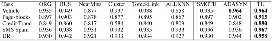
Table 3: Performance of the proposed method TU and prevailing data sampling methods on the tested real-world datasets. Here, RUS refers to the random undersampling method. The second group of methods are all undersampling-based and the third group of methods are all oversampling-based.

Task ORG RUS NearMiss Cluster TomekLink ALLKNN SMOTE ADASYN TU

Vehicle 0.935 0.949 0.877 0.937 0.938 0.858 0.935 0.964 0.964

Page-blocks 0.897 0.903 0.878 0.877 0.895 0.867 0.897 0.902 0.915

Credit Fraud 0.849 0.860 0.817 0.584 0.840 0.809 0.849 0.848 0.880

SMS Spam 0.936 0.938 0.931 0.932 0.935 0.933 0.936 0.936 0.967

DR 0.930 0.942 0.921 0.933 0.934 0.927 0.930 0.944 0.958

with 25 units for the other tasks. For the SMS Spam task, we reduced the input dimension to 100 with PCA for the policy network. For the DR task, we used the publicly available network architecture and weights provided by a participant who scored very well in the Kaggle DR competition, which we will call JFnet (Fauw 2015), as the classifier. And we re-trained its last two fully connected layers on each sampled dataset.

We first compared the proposed method against pre-vailing data sampling methods. These methods include six undersampling methods, i.e.,Random Majority Under-sampling(RUS), Near Miss(NearMiss) (Mani and Zhang 2003), Cluster Centroid (Cluster) (Lemaˆıtre, Nogueira, and Aridas 2017), TomekLink (Tomek 1976b), and AL-LKNN (Tomek 1976a), and two oversampling methods, i.e.,SMOTE(Chawla et al. 2002) and ADASYN (He et al. 2008). All of them were implemented using imbalanced-learn (Lemaˆıtre, Nogueira, and Aridas 2017).

Table 3 lists the comparison results on the five real-world datasets. From the table, We can obtain the following observations.1)The performance of the prevailing heuristic-based data sampling methods varies considerably by dataset. None of them can consistently outperform other heuristic-based data sampling methods. This shows the drawbacks of these method that their applicabilities are limited to specific dataset. 2) Our proposed data sampling method TU can consistently outperforms the heuristic-based data sampling methods, showing its robustness and effectiveness.

We further compared the proposed method with some state-of-the-art methods, though they may be inapplicable to some tasks. These methods includeEasyEnsemble(Liu, Wu, and Zhou 2009), BalanceCascade (Liu, Wu, and Zhou 2009), EUS (Garc´ıa and Herrera 2009), and cost-sensitive learning (Parambath, Usunier, and Grandvalet 2014). Note that we replace the 1NN model of EUS with the corresponding used classifier for each dataset. In

addition, we compare with the model-level evaluation metric optimization method using reinforcement learning (RL) (Wu et al. 2016), which we refer toRL.

Table 4 lists the results of these baselines compared to our proposed method. Results of the cost-sensitive method on the Vehicle and Credit Fraud tasks are missing because there are no published methods for the implementation on the used evaluation metrics. Result of the BalanceCascade method on the DR task is missing because the computation cost is too large, and results of the RL method on the Vehicle and Credit Fraud tasks are missing because it is not applicable to the used classifiers. From the table we can see that our proposed method can achieve comparable performance with state-of-the-art methods. Note that, though the cost-sensitive methods perform slightly better than our propose method on some tasks, they need specific designation for the given evaluation metric and cannot generally transform to other measurements. In the meanwhile, the RL method suffers the problem that cannot apply to non-parametric classifiers. In contrast, our proposed method can easily apply to arbitrary evaluation metric and classifier.

In addition, according to our aforementioned discussion in the Related Work section, the proposed method, as a meta-learning approach, can also collaborate with other data-level operations. Here, we study the applicability of the proposed to incorporate with the oversampling methods. This can also assess if the oversampling methods can create new informative instances instead of just changing the data distribution.

(7)

Table 4: Comparison of our proposed method with state-of-the-art class-imbalance learning methods on the tested real-world datasets. Some results of these methods are missing because there are no published methods for the implementation or the computation cost is too large, or the method is not applicable to the used classifier. Cost-sensitive methods are implemented according to their referenced paper, respectively.

Task CostSensitive EasyEnsemble BalanceCascade EUS RL TU

Vehicle − − − 0.953 0.955 0.960 − − − 0.964

Page-blocks 0.916(2007) 0.904 0.901 0.907 0.916 0.915

Credit Fraud − − − 0.859 0.865 − − − − − − 0.880

SMS Spam 0.964 (2014) 0.939 0.935 0.965 0.962 0.967

DR 0.950 (2007) 0.945 − − − − − − 0.958 0.958

Table 5: Results of the proposed method incorporating with the oversampling technique. SMOTE+TU is to oversample the dataset using SMOTE and then apply the proposed method to the oversampled dataset.

Task ORG SMOTE ADASYN TU SMOTE+TU ADASYN+TU

Vehicle 0.935 0.964 0.964 0.964 0.964 0.965

Page-blocks 0.897 0.902 0.898 0.915 0.917 0.915 Credit Fraud 0.849 0.848 0.849 0.880 0.881 0.880

SMS Spam 0.936 0.936 0.936 0.967 0.965 0.967

DR 0.930 0.944 0.943 0.958 0.957 0.956

0 100 200 300 400 500 600 700 800 900 Time (s)

0.89 0.90 0.91 0.92 0.93 0.94 0.95 0.96 0.97

GM

RUS EUS

(a) Vehicle

0 1000 2000 3000 4000 5000 6000 Time (s)

0.84 0.85 0.86 0.87 0.88 0.89 0.90 0.91 0.92

MCC

RUS

(b) Page blocks

0 20000 40000 60000 80000 100000 120000 140000 160000 Time (s)

0.845 0.850 0.855 0.860 0.865 0.870 0.875 0.880 0.885

AUCPRC RUS

(c) Credit Fraud

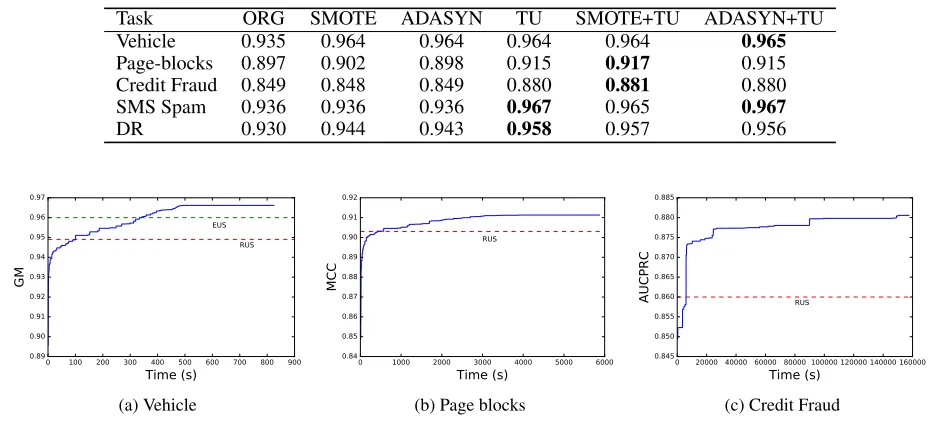
Figure 2: Time complexity of the proposed method on three tested datasets. The red dot line denotes the performance of the random undersampling method.

distribution. Therefore, the optimum subset for the given classier chosen from the oversampled dataset is similar to that chosen from the original training dataset.

Finally, we empirically study the time complexity of the proposed method on the tested datasets. Figure 2 depicts the training process of the proposed method by time (second) on three tested datasets using a single GPU. From the figure, we can see that the proposed method can quickly outperform the random undersampling method and achieve further improvement.

Conclusion

In this work, we propose a trainable undersampling method. It incorporates the evaluation metric optimization into the data sampling procedure thus can learn which in-stances should be discarded and which inin-stances should be preserved. Moreover, as a data level operation, it can easily apply to arbitrary evaluation metric and classifier, including the non-parametric ones. Empirical studies on

several synthetic and realistic datasets show that this method can consistently outperform prevailing heuristic-based data sampling methods and achieve better results than the state-of-the-art methods in most of cases.

Acknowledgments

The authors wish to thank the anonymous reviewers for their helpful comments. This work was partially funded by China National Key R&D Program (No. 2017YFB1002104, 2018YFC0831105), National Natural Science Foundation of China (No. 61532011, 61751201, 61473092, and 61472088), and STCSM (No.16JC1420401,17JC1420200).

References

Bahdanau, D.; Cho, K.; and Bengio, Y. 2014. Neural machine translation by jointly learning to align and translate. arXiv preprint arXiv:1409.0473.

(8)

training data. ACM SIGKDD explorations newsletter6(1):20– 29.

Błaszczy´nski, J., and Stefanowski, J. 2015. Neighbourhood sampling in bagging for imbalanced data. Neurocomputing

150:529–542.

Calders, T., and Jaroszewicz, S. 2007. Efficient auc optimization for classification. In European Conference on Principles of Data Mining and Knowledge Discovery, 42–53. Springer.

Chawla, N. V.; Bowyer, K. W.; Hall, L. O.; and Kegelmeyer, W. P. 2002. Smote: synthetic minority over-sampling technique. Journal of artificial intelligence research16:321– 357.

Cieslak, D. A., and Chawla, N. V. 2008. Start globally, optimize locally, predict globally: Improving performance on imbalanced data. In Data Mining, 2008. ICDM’08. Eighth IEEE International Conference on, 143–152. IEEE.

Dal Pozzolo, A.; Caelen, O.; Johnson, R. A.; and Bontempi, G. 2015. Calibrating probability with undersampling for unbalanced classification. InComputational Intelligence, 2015 IEEE Symposium Series on, 159–166. IEEE.

Eban, E.; Schain, M.; Mackey, A.; Gordon, A.; Rifkin, R.; and Elidan, G. 2017. Scalable learning of non-decomposable objectives. InArtificial Intelligence and Statistics, 832–840. Fauw, D. 2015. J. 5th place solution of the kaggle diabetic retinopathy competition.

Fern´andez, A.; Garc´ıa, S.; del Jesus, M. J.; and Herrera, F. 2008. A study of the behaviour of linguistic fuzzy rule based classification systems in the framework of imbalanced data-sets.Fuzzy Sets and Systems159(18):2378–2398.

Ganganwar, V. 2012. An overview of classification algorithms for imbalanced datasets. International Journal of Emerging Technology and Advanced Engineering2(4):42–47.

Garc´ıa, S., and Herrera, F. 2009. Evolutionary undersampling for classification with imbalanced datasets: Proposals and taxonomy. Evolutionary computation17(3):275–306.

Hanley, J. A., and McNeil, B. J. 1982. The meaning and use of the area under a receiver operating characteristic (roc) curve.

Radiology143(1):29–36.

He, H., and Garcia, E. A. 2009. Learning from imbalanced data. IEEE Transactions on knowledge and data engineering

21(9):1263–1284.

He, H.; Bai, Y.; Garcia, E. A.; and Li, S. 2008. Adasyn: Adaptive synthetic sampling approach for imbalanced learning. InNeural Networks, 2008. IJCNN 2008.(IEEE World Congress on Computational Intelligence). IEEE International Joint Conference on, 1322–1328. IEEE.

Herschtal, A., and Raskutti, B. 2004. Optimising area under the roc curve using gradient descent. InProceedings of the twenty-first international conference on Machine learning, 49. ACM. Kang, P., and Cho, S. 2006. Eus svms: Ensemble of under-sampled svms for data imbalance problems. In

International Conference on Neural Information Processing, 837–846. Springer.

Leibig, C.; Allken, V.; Ayhan, M. S.; Berens, P.; and Wahl, S. 2017. Leveraging uncertainty information from deep neural networks for disease detection.Scientific reports7(1):17816.

Lemaˆıtre, G.; Nogueira, F.; and Aridas, C. K. 2017. Imbalanced-learn: A python toolbox to tackle the curse of imbalanced datasets in machine learning. Journal of Machine Learning Research18(17):1–5.

Liu, X.-Y.; Wu, J.; and Zhou, Z.-H. 2009. Exploratory undersampling for class-imbalance learning. IEEE Transac-tions on Systems, Man, and Cybernetics, Part B (Cybernetics)

39(2):539–550.

Mani, I., and Zhang, I. 2003. knn approach to unbalanced data distributions: a case study involving information extraction. In Proceedings of workshop on learning from imbalanced datasets, volume 126.

Matthews, B. W. 1975. Comparison of the predicted and observed secondary structure of t4 phage lysozyme.Biochimica et Biophysica Acta (BBA)-Protein Structure405(2):442–451. Norouzi, M.; Bengio, S.; Jaitly, N.; Schuster, M.; Wu, Y.; Schuurmans, D.; et al. 2016. Reward augmented maximum likelihood for neural structured prediction. In Advances In Neural Information Processing Systems, 1723–1731.

Parambath, S. P.; Usunier, N.; and Grandvalet, Y. 2014. Optimizing f-measures by cost-sensitive classification. In

Advances in Neural Information Processing Systems, 2123– 2131.

Pedregosa, F.; Varoquaux, G.; Gramfort, A.; Michel, V.; Thirion, B.; Grisel, O.; Blondel, M.; Prettenhofer, P.; Weiss, R.; Dubourg, V.; Vanderplas, J.; Passos, A.; Cournapeau, D.; Brucher, M.; Perrot, M.; and Duchesnay, E. 2011. Scikit-learn: Machine learning in Python. Journal of Machine Learning Research12:2825–2830.

Ranzato, M.; Chopra, S.; Auli, M.; and Zaremba, W. 2015. Sequence level training with recurrent neural networks. arXiv preprint arXiv:1511.06732.

Tieleman, T., and Hinton, G. 2012. Lecture 6.5-rmsprop: Divide the gradient by a running average of its recent magnitude. COURSERA: Neural networks for machine learning4(2):26–31.

Tomek, I. 1976a. An experiment with the edited nearest-neighbor rule. IEEE Transactions on systems, Man, and Cybernetics(6):448–452.

Tomek, I. 1976b. Two modifications of cnn. IEEE Trans. Systems, Man and Cybernetics6:769–772.

Van Hulse, J.; Khoshgoftaar, T. M.; and Napolitano, A. 2007. Experimental perspectives on learning from imbalanced data. InProceedings of the 24th international conference on Machine learning, 935–942. ACM.

Williams, R. J. 1992. Simple statistical gradient-following algorithms for connectionist reinforcement learning. In

Reinforcement Learning. Springer. 5–32.

Wilson, D. L. 1972. Asymptotic properties of nearest neighbor rules using edited data. IEEE Transactions on Systems, Man, and Cybernetics(3):408–421.

Wu, Y.; Schuster, M.; Chen, Z.; Le, Q. V.; Norouzi, M.; Macherey, W.; Krikun, M.; Cao, Y.; Gao, Q.; Macherey, K.; et al. 2016. Google’s neural machine translation system: Bridging the gap between human and machine translation.