The Thirty-Third AAAI Conference on Artificial Intelligence (AAAI-19)
Structured Bayesian Networks: From Inference to Learning with Routes
Yujia Shen, Anchal Goyanka, Adnan Darwiche, Arthur Choi
Computer Science DepartmentUniversity of California, Los Angeles {yujias,anchal,darwiche,aychoi}@cs.ucla.edu
Abstract
Structured Bayesian networks (SBNs) are a recently proposed class of probabilistic graphical models which integrate back-ground knowledge in two forms: conditional independence constraints and Boolean domain constraints. In this paper, we propose the first exact inference algorithm for SBNs, based on compiling a given SBN to a Probabilistic Sentential De-cision Diagram (PSDD). We further identify a tractable sub-class of SBNs, which have PSDDs of polynomial size. These SBNs yield a tractable model of route distributions, whose structure can be learned from GPS data, using a simple algo-rithm that we propose. Empirically, we demonstrate the utility of our inference algorithm, showing that it can be an order-of-magnitude more efficient than more traditional approaches to exact inference. We demonstrate the utility of our learning al-gorithm, showing that it can learn more accurate models and classifiers from GPS data.
1
Introduction
Structured Bayesian Networks (SBNs) were recently pro-posed by (Shen, Choi, and Darwiche 2018) for representing and learning distributions over highly complex spaces, such as routes on a map. Like a Bayesian network (BN), an SBN is defined by a directed acyclic graph (DAG) and a set of conditional distributions. In contrast to a BN, each node of an SBN represents aclusterof variables (not just a single variable). Thiscluster DAG specifies conditional indepen-dencies betweensetsof variables, but makes no claims about the independencies between variables in the same cluster. Also in contrast to a BN, which uses tabular CPTs to rep-resent conditional distributions, an SBN uses a conditional Probabilistic Sentential Decision Diagram, or conditional PSDD, to compactly represent the distribution over a cluster, conditioned on its parent clusters (Shen, Choi, and Darwiche 2018). SBNs can hence accommodate background knowl-edge in the form of conditional independence constraints (via the cluster DAG), as well as knowledge in the form of Boolean domain constraints (via the conditional PSDD).
Initially, (Shen, Choi, and Darwiche 2018) proposed an efficient, closed-form algorithm for estimating the parame-ters of an SBN from complete data. However, they left open the problem of performing inference in an SBN, once it has
Copyright c2019, Association for the Advancement of Artificial Intelligence (www.aaai.org). All rights reserved.
been learned from data. In this paper, we propose the first exact inference algorithm for SBNs, which is based on com-piling them to a Probabilistic Sentential Decision Diagram (PSDD) (Kisa et al. 2014). Our algorithm is based on the compilation algorithm of (Shen, Choi, and Darwiche 2016), for compiling Bayesian networks into PSDDs.
In general, compiling an SBN to a PSDD is not al-ways tractable. However, we identify a new sub-class of SBNs that is guaranteed to have PSDDs ofpolynomialsize. These SBNs have applications in modeling distributions over routes (Zheng 2015; Choi, Shen, and Darwiche 2017). Next, we propose a new structure learning algorithm for this tractable class of SBNs. On the inference side, we show our algorithm can be an order-of-magnitude more efficient than more traditional approaches to exact inference. On the learn-ing side, we show that we can learn more effective models for the tasks of route prediction and route classification.
This paper is structured as follows. In Section 2, we re-view SBNs and PSDDs. Next, in Section 3, we propose our algorithm for compiling SBNs to PSDDs. We identify a tractable sub-class of SBNs in Section 4, whose PSDDs have polynomial size. We propose our learning algorithm in Section 5. Finally, we provide an empirical analysis in Sec-tion 6 and conclude in SecSec-tion 7.
2
Structured Bayesian Networks
The Structured Bayesian network (SBN) is a recently pro-posed class of probabilistic graphical model which is capa-ble of integrating background knowledge in the form of both conditional independence constraints and Boolean domain constraints (Shen, Choi, and Darwiche 2018).To specify an SBN, one first defines acluster DAG. As a Bayesian network’s structure is defined by a DAG, a Struc-tured Bayesian network’s structure is defined by its cluster DAG, where each node represents asetof random variables (a cluster). The cluster DAG represents conditional dencies between these sets of variables: a cluster is indepen-dent of its non-descendant clusters given its parent clusters. Importantly, nothing is said in terms of independence be-tween variables of the same cluster, which is less commit-ting than the DAG of a Bayesian network. In a cluster DAG, we refer to a clusterXand its parentsPas afamilyX|P.
A B C P r
0 0 0 0.2
0 0 1 0.2
0 1 0 0.0
0 1 1 0.1
1 0 0 0.0
1 0 1 0.3
1 1 0 0.1
1 1 1 0.1
(a) Distribution
A B¬A¬B A¬B¬A B
1 4 1
C¬C
C
3
(b) An SDD
A B¬A¬B A¬B¬A B
1
.33 .67
1
.75 .25 4
C¬C .5 .5
C
3
.6 .4
(c) A PSDD
A
B
C
31
0 2
4
(d) A vtree
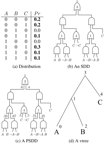
Figure 1: A probability distribution and its SDD/PSDD rep-resentation. The numbers annotating or-gates in (b) & (c) correspond to vtree node IDs in (d). Moreover, while the cir-cuit appears to be a tree, the input variables are shared and hence the circuit is not a tree.
PSDD, which defines the conditional distribution of a cluster given its parent clusters. The conditional PSDD is composed of two components: (1) the logical constraints that define the feasible states of a cluster given the states of its parent clusters, and (2) the parameters that are learned from data. We review PSDDs and conditional PSDDs next.
Probabilistic Sentential Decision Diagrams
PSDDs were motivated by the need to represent probabil-ity distributionsPr(X)with many instantiationsxattaining zero probability,Pr(x) = 0(Kisa et al. 2014). Consider the distributionPr(X)in Figure 1a for an example. The first step in constructing a PSDD for this distribution is to con-struct a special Boolean circuit that captures its zero entries; see Figure 1b, which was compiled automatically from the logical constraints (the zeros). The Boolean circuit captures zero entries in the following sense. For each instantiationx, the circuit evaluates to0 at instantiationxiffPr(x) = 0. The second and final step of constructing a PSDD amounts to parameterizing this Boolean circuit (e.g., by learning from data), which adds a local distribution on the inputs of each or-gate; see Figure 1c.
This annotated circuit induces a distribution Pr(X) as follows. First, the probability of a complete instantiationx is obtained by performing a bottom-up pass, evaluating each
p1 s1 p2 s2
· · ·
pnsn
· · ·
α1
α2
αn
Figure 2: SDD fragment
gate from the inputs to the output. An input evaluates to1or
0depending on its value set byx. The value of an and-gate is the product of the values of its inputs. The value of an or-gate is the weighted sum of its inputs (using the weights annotating the inputs). Finally,P
xPr(x) = 1.For more on
the semantics of PSDDs, see (Kisa et al. 2014).
The Boolean circuit underlying a PSDD is known as a Sentential Decision Diagram (SDD) (Darwiche 2011). An SDD circuit is constructed from the fragment in Figure 2, where or-gates can have any number of inputs, and and-gates have two inputs each. Eachpi is called aprime and each si is called a sub.Each SDD circuit conforms to a tree of
variables called avtree, which is a binary tree whose leaves are the circuit variables; see Figure 1d. The conformity is roughly as follows. For each SDD fragment with primespi
and subssi, there exists a vtree nodevwhere the variables
of SDDpi are those of the left child ofv and the variables
of SDD si are those of the right child of v. For the SDD
in Figure 1b, each or-gate has been labeled with the ID of the vtree node it conforms to. For example, the top fragment conforms to the vtree root (ID=3), with its primes having variables{A, B}and its subs having variables{C}. Finally, when the circuit is evaluated underanyinput, precisely one prime pi of each fragment will be1. Hence, the fragment
output will simply be the value of the corresponding subsi.1
A PSDD can now be obtained by annotating a distribution
α1, . . . , αnon the inputs of each or-gate, wherePiαi= 1.
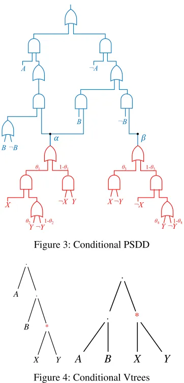
Aconditional PSDDrepresents asetof distributions over variablesX, which are conditioned on thesameset of vari-ablesP. A conditional PSDD is motivated by the need to represent the conditional distributionsPr(X|P)of a clus-ter, in a cluster DAG, whereXare the variables of the clus-ter andPare the variables of its parent clusters (Shen, Choi, and Darwiche 2018). A conditional PSDD can be viewed as having two components: a PSDD component that repre-sents each conditional distributionPr(X|p), and an SDD component that serves to index these distributions based on the parent instantiationp. A conditional PSDD can also ag-gregate common conditional distributions, particularly when there is significantcontext-specific independence(Boutilier et al. 1996). For example, consider the conditional PSDD in Figure 3, whereαandβdenote two PSDDs highlighted in red, with the SDD component highlighted in blue. The PSDD forαis shared among all parent instantiations where
1
A
B
X
θ1 1-θ1
θ2 1-θ2 θ4 1-θ4
θ3 1-θ3 ! "
¬A
¬B
B ¬B
¬X Y X¬Y ¬X
¬Y Y ¬Y
Y
Figure 3: Conditional PSDD
.
A .
B *
X Y
.
. *
A
B
X
Y
Figure 4: Conditional Vtrees
AorBis true. The PSDD forβis obtained by a single par-ent instantiation, whereAandBare both false. For more on conditional PSDDs, see (Shen, Choi, and Darwiche 2018).
Vtrees
In the compilation algorithm that we propose next, the con-ditional vtree and the decision vtreewill be central. First, for an internal vtree nodev, we refer tovlandvras the left and right children ofv. We call an internal vtree nodev a Shannon nodeiff its left child is a leaf node. Consider the following definition of a decision vtree, originally proposed by (Oztok, Choi, and Darwiche 2016).
Definition 1 (Decision Vtree) A familyX | Pis compat-ible with an internal vtree node v iff the family has some variables mentioned invland some variables mentioned in vr. A vtree for an SBNNis said to be a decision vtree forN
iff every family inNis compatible with only Shannon nodes.
Next, we consider conditional vtrees. Any conditional PSDD must conform to a conditional vtree.
Definition 2 (Conditional Vtrees) Letvbe a vtree for vari-ablesX∪P which has a node u that contains precisely the variables X. If node u can be reached from node v
by only following right children, then v is said to be a conditional vtree forX|Panduis said to be itsX-node.
Figure 4 depicts two examples of conditional vtrees for X ={X, Y} andP = {A, B}. TheX-nodes are starred. The vtree under the X-node determines the circuit struc-ture of the probabilistic (PSDD) component of a conditional PSDD. In turn, the vtree outside of theX-node determines the circuit structure of the logical (SDD) component.
Finally, we say that two vtrees, one over variablesXand the other over variablesY,are compatible iff they can be ob-tained by projecting some other common vtree on variables XandY, respectively.
Definition 3 (Vtree Projection) Letvbe a vtree over vari-ablesZ.The projection ofvon variablesX⊆Zis obtained as follows. Successively remove every maximal subtree v0
whose variables are outsideX,while replacing the parent ofv0with its sibling.
3
Exact Inference by Compilation to PSDDs
In this section, we propose the first exact inference algorithm for Structured Bayesian networks (SBNs). Our approach is based on the approach proposed by (Shen, Choi, and Dar-wiche 2016), for compiling Bayesian networks into PSDDs, which we summarize below:1. pick a decision vtreev for the given Bayesian network
N, using min-fill for example;
2. compile each CPT of networkN into a PSDD using the vtreevprojected onto the CPT’s variables;
3. using the PSDD multiply operator, multiply all CPTs.
The result is a single PSDD representing the joint distribu-tion of the given BN; we shall refer to this PSDD as the joint PSDD. Once we obtain the joint PSDD, we can per-form exact inference efficiently: we can compute marginals or MPEs, for example, in time linear in the size of the PSDD (Kisa et al. 2014). Moreover, one can bound the size of the joint PSDD of a BN by its treewidth, by using an appropriate vtree (Shen, Choi, and Darwiche 2016).
To perform exact inference in SBNs, we also perform three similar steps, with Step (3) being the same for SBNs as it is for BNs: each conditional PSDD can be treated as a PSDD, which we can multiply together. Step (1) is also similar for SBNs, but we will need another method for pick-ing a special type of vtrees for SBNs, which we discuss later. Step (2) is the main difference. In order to multiply two PSDDs together using the PSDD multiply operator, the vtrees of the two PSDDs must be compatible, i.e., they are the projections of the same vtree (Shen, Choi, and Darwiche 2016).2 This is easy to ensure in a BN, as we simply
con-vert each CPT to a PSDD using the vtree from Step (1). This is not easy to ensure in an SBN, since their conditional dis-tributions must be specified as a conditional PSDD already, whose conditional vtrees may not be compatible.3 Hence,
2
Given two PSDDs with compatible vtrees, of sizess1ands2,
the complexity of multiplication isO(s1s2).
3
Algorithm 1ConstructDecisionCtree(cluster DAGB, topo-logical orderingπ)
1: ifBis a single clusterXthen returna leaf ctree for clusterX
2: else ifBis disconnectedthen
3: B1,B2←a disconnected partition ofB
4: π1, π2 ←sub-orders over clusters inB1,B2 of the total
orderingπ
5: else
6: X←first cluster of orderingπ
7: B1,B2 ←root clusterX, and cluster DAG Bwith root
clusterXremoved
8: π1, π2 ←orderinghXi, and orderingπwith the first
ele-mentXremoved
9: vl←ConstructDecisionCtree(B1, π1).
10: vr←ConstructDecisionCtree(B2, π2).
11: returna ctreevwith with left and right childrenvlandvr
for SBNs, in Step (1), we need to make sure we pick the right vtree that will allow us to, in Step (2), enforce compat-ibility. We discuss how to do this next.
Finding a Global Vtree
In this section, we consider analogues of vtrees (and their variations) for SBNs, where leaves are labeled by clusters of the SBN, rather than by variables; we refer to these cluster trees asctrees. A ctree can be viewed as a restricted type of vtree: a ctree is a vtree where the variables Xof a cluster appear in the same sub-vtree, but where we represent this sub-vtree with a single leaf ctree node. Note, however, that we shall leave the sub-vtree over variables Ximplicit for now, and first show how to pick a ctree.
Our goal is to identify a ctree for a given SBN that will ac-commodate inference by PSDD multiplication. The first re-quirement is that the ctrees of all conditional PSDDs must be compatible with some common joint ctree. The second re-quirement is that these ctrees must also be conditional ctrees. The first requirement can be enforced by insisting that our ctree be adecision ctreewith respect to our SBN. The sec-ond requirement can be enforced, in addition to using a deci-sion ctree, by restricting the decideci-sion ctree to respect a topo-logical ordering. In this case, the child cluster is guaranteed to appear as the right-most leaf in the ctree (which guaran-tees a conditional ctree). Algorithm 1 provides an algorithm for finding such a ctree, given a cluster DAG and a topo-logical ordering of its clusters. The following proposition summarizes the result.
Proposition 1 The ctreevreturned by Algorithm 1 is a de-cision ctree with respect to the input cluster DAG. Moreover, for each familyX|Pin the cluster DAG, the projection of
vonto familyX|Pis a conditional ctree for the family.
This ctree and its implied conditional ctrees can be used to perform exact inference in an SBN via compilation.
How-In an SBN, conditional PSDDs represent complex conditional dis-tributions that would otherwise have intractable representations as tables; hence, a conditional PSDD must typically be learned from data directly. In addition, when learning conditional PSDDs, we will want to learn their conditional vtrees independently (to pro-vide the best fit to the data).
A1A2A3
C1C2 B1B2
(a) Cluster DAG
A1
A2 A3
★
•
(b) Vtree for clusterA
B
1
B
2
★
(c) Vtree for clusterB
A1 A2
A3
•
• B1 B2
• •
•
★
C1 C2
(d) Vtree for clusterC
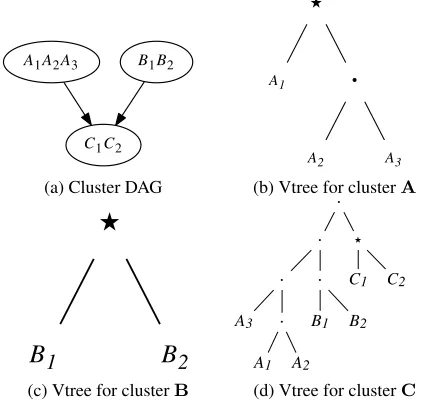
Figure 5: A cluster DAG and three conditional vtrees for clusters A = {A1, A2, A3}, B = {B1, B2}, and C =
{C1, C2}.X-nodes are labeled with a star.
ever, we must first show how to choose the sub-vtrees over the variablesXof a cluster, which we do next.
Finding Local Vtrees
Typically, when learning PSDDs from data, one must also learn its vtree (Liang, Bekker, and Van den Broeck 2017; Shen, Choi, and Darwiche 2017). In an SBN, it suffices to learn the conditional PSDDs of its conditional distributions (Shen, Choi, and Darwiche 2018). To provide the best fit, we should learn the corresponding conditional vtrees in-dependently. However, to perform inference, these condi-tional vtrees must be compatible, as projections of a com-mon global vtree. We show how to achieve this next.
Consider the cluster DAG of Figure 5, and its three con-ditional vtrees. Here, the vtree for clusterAis not compat-ible with the vtree for clusterC, as their projections onto variablesAare different vtrees. More generally, consider a familyX | Pand its conditional vtreev. Letudenote the X-node ofv. Sub-vtreeudictates the probabilistic (PSDD) component of a conditional PSDD, whereas the sub-vtree outside ofu,overP,dictates the logical (SDD) component. That is, the distribution induced by a conditional PSDD de-pends only on the sub-vtreeuoverX. The sub-vtree overP impacts the size of the conditional PSDD but not its distribu-tion. We thus propose to manipulate the conditional vtrees of an SBN so that they become compatible, but for each family X|Pwith conditional vtreevandX-nodeu, we leave the sub-vtreeufixed inv. In this case, the probabilistic (PSDD) components of each conditional PSDD will also be fixed, leaving the conditional distributions invariant.
exact inference via compilation. Our first step is to obtain a target decision ctreev,where each conditional vtree will be made compatible withv. We first run Algorithm 1 to obtain a decision ctreecfor our SBN. For each familyX|P, we then replace the leaf clusterXin ctreecwith theX-node of the family’s conditional vtree, yielding our target vtreev.
Our second step is to adjust all conditional vtrees so that it is compatible with v. More specifically, for each fam-ily X | P, we adjust the logical (SDD) component of its conditional vtree/PSDD, through a process called re-normalization.4Tree rotation and swap operators were
pre-viously used to re-normalize an SDD to a new vtree (Choi and Darwiche 2013), where an operation on the vtree im-plied a corresponding re-factorization of the logical circuit of the SDD.5 After re-normalization, the resulting
condi-tional PSDDs are now all compatible with each other.
4
A Tractable Class of SBNs
We identify a tractable sub-class of SBNs, which can be compiled into joint PSDDs with only polynomial size— namely those that correspond tobinary hierarchical maps. This class of SBNs are of practical interest, as they are in-spired from an application of SBNs for modeling distribu-tions over routes on a map, or equivalently, simple paths on a graph (Zheng 2015; Choi, Shen, and Darwiche 2017).
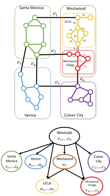
Consider in Figure 6, a simplified graph of neighborhoods in the Los Angeles Westside, where edges represent streets and nodes represent intersections. The nodes of the LA Westside have been partitioned into four sub-regions: Santa Monica, Westwood, Venice and Culver City. Westwood is further partitioned into two smaller sub-regions: UCLA and Westwood Village. This partitioning is an example of a hier-archical map, or more simply, anhmap. An hmap allows one to abstract the notion of a route in a map: an abstract route is a route between regions, which can be refined by recur-sively planning the routes in each region. For example, if we want to go from Venice to Westwood, we may first decide to use edgee4to go from Venice to Santa Monica, and then
use edgee1 to go from Santa Monica to Westwood. Next,
we find a route in Venice to edgee4, then a route through
Santa Monica from edgee4toe1, and finally a route in
West-wood frome1to the destination (we can then recursively find
routes between UCLA and Westwood Village).
An hmap induces a cluster DAG as follows; see Figure 6. Each node of this cluster DAG represents a region, and each edge of the cluster DAG indicates that the child is a sub-region of the parent. Each node of the cluster DAG is as-sociated with the map edges that are used at that level; for
4
For a familyX|P,letwbe its conditional PSDD, and letv0
be the projection of decision vtreevontoX|P. First, we extract the SDD circuit of a conditional PSDD. For both vtreeswandv0, we replace the leaf clusterXwith a dummy leaf vtree; we also replace the corresponding PSDD nodes of the conditional PSDD with dummy terminals. We then re-normalize the resulting (alge-braic) SDD so that it conforms tov0instead ofw,and replace the dummy terminals with the original PSDD nodes.
5
To re-normalize an SDD, it also suffices to re-construct the SDD bottom-up for the new vtree, using the SDD’sapply opera-tor (Darwiche 2011), which we did in our experiments.
Venice
Westwood Santa Monica
Culver City
e1
e2
e3 e4
e5 e6
UCLA
w1
v1 v2
v3 v4 u7
u1
u2 u3 u4
u5 u6
Westwood Village
Venice
n1,...,n6
Santa Monica
s1,...,s8
Culver City
c1,...,c6
UCLA
u1,...,u7
Westside
e1,...,e6
Westwood Village
v1,...,v4
Westwood
w1
Figure 6: A hierarchical map and its cluster DAG.
an internal node, they are the edges that are used to cross between the child sub-regions. Here, the root cluster repre-sents the LA Westside and its variables represent the edges
e1, . . . , e6 that are used to cross between its four
(imme-diate) sub-regions. Finally, each leaf cluster represents the edges that are strictly contained in that sub-region. Consider the conditional independencies implied by a cluster DAG: given the edges used to enter a region, the route that we take inside of a region is independent of the route taken outside the region. We make an additional assumption, due to (Choi, Shen, and Darwiche 2017), which we also exploit: the route taken inside of a region must also be a simple path.
In a binary hmap, regions are recursively split into two sub-regions. Such maps have three key properties, that lead to its tractability: (1) the simple-path constraints for interior nodes are trivial to compile,6 (2) the number of parent in-stantiations that we need to consider in a conditional PSDD is quadratic in the number of edges crossing into the region,7
and (3) if the simple-path constraints of a leaf region are too
6
A path consists of crossing from one region to another using a single edge, or not at all, because of the simple path assumption (in a simple path, we cannot visit the same region twice).
7
hard to compile, we can make the map deeper until they are compilable. With a binary hmap, we obtain the following polynomialbound on the size of its joint PSDD.
Theorem 1 Consider a binary hmap withtnodes, wherek
is the maximum number of edges assigned to a cluster and
nis the maximum number of edges that cross into a region. Letmdenote the size of the largest PSDD of any leaf region. The size of the joint PSDD isO(t·n2·(m+k)).
A proof is included in the Appendix.
5
Learning Binary Hierarchical Maps
In this section, we consider how to learn a binary hmap, and hence, the structure of an SBN.Random Binary Hmaps.Consider the following simple algorithm for inducing a random binary hmap, based on re-cursively decomposing a map into two regions. First, pick two seed nodesaandbof a map, whereawill belong to one region andbwill belong to the other. Each region alternates between absorbing a neighboring node into their region (if possible), until all nodes are absorbed. A deeper hmap can then be produced by recursing on the sub-regions. We typ-ically recurse until each leaf region is small enough to be compilable to an SDD.
Learning Hmaps from Data.We next propose a heuris-tic for learning a binary hierarchical map from a dataset con-sisting of routes. Consider a popular road on a map which is used by many routes in the data. A random partitioning of the map may put one intersection (node) of the road in one region, the next intersection in another region, and the third intersection in the same region as the first. Hence, a route on this road would exit the first region, enter the second, and then re-enter the first. Such a route is not simple relative to an hmap as it visits the same region twice. This assumption was introduced by (Choi, Shen, and Darwiche 2017), and is important for guaranteeing tractability as we discussed in the previous section.
Hence, we propose a heuristic that tries to avoid situa-tions like the above, for learning a binary hmap from data. Our approach is bottom-up.8 Intuitively, we want to
clus-ter nodes together if they are commonly used by the same route. First, we assign each node to its own region. Next, we have an edge between regions if there is a street connecting them, and we give that edge a weight based on the number of routes in the data that crosses from one region to the other. We then find a maximum weight matching9and merge each
of the paired regions. We update the scores between regions and repeat, until we obtain a single cluster. Next, from the clustering, we want to extract an hmap whose leaf regions are as large as possible, given an upper limit. Hence, to ob-tain our final hmap, we navigate the clustering in depth-first fashion until we find the first node under our limit which we take as an hmap leaf. We then backtrack and continue until we have picked all of our leaves.
edges can be used).
8
Essentially, learning a binary hmap is a type of hierarchical clustering. See, e.g., (Murphy 2012) which discusses both bottom-up (agglomerative) and top-down (divisive) clustering.
9
We used thenetworkxpython module.
Figure 7: The road network of downtown SF.
6
Empirical Evaluation
We now evaluate the inference and learning algorithms we proposed for SBNs. First, we compare inference using PS-DDs with a baseline using jointree inference with sparse ta-bles. Next, we evaluate the quality of SBNs learned using our proposed heuristic, in a route prediction task. Finally, we highlight the utility of SBN models for route classification.
Efficiency of Exact Inference.First, we compare the ef-ficiency of our exact inference algorithm for SBNs, with jointree message-passing using sparse tables (Larkin and Dechter 2003).10We evaluate these inference algorithms on an SBN induced from a hmap, as done by (Choi, Shen, and Darwiche 2017). We obtained public map data of San Fran-cisco (SF) from openstreetmap.org, and selected7 increas-ingly larger regions of SF. We induced a random binary hmap from each map, as described in Section 5. For each map size, we generated5×5×5 = 125problem instances: (1)5random hmaps, (2)5random parameterizations of the SBN, and (3)5MPE queries (what is the most likely route between randomly chosen source/destination pairs). In Ta-ble 1, we report averages and standard deviations for the times to (1) compile the joint PSDD (offline step), (2) eval-uate the PSDD (online query step), and (3) run the jointree algorithm. For each region, the graph size reported is the number of edges (road segments) in the map, and depth is the average depth of the binary hmap.
The largest map considered had10,500edges; its graph is highlighted in Figure 7. On average, the corresponding SBN had 1.7M parameters and the joint PSDD was of size 8.9M (edges). Note that this map is over 26 times larger than the map considered by (Choi, Shen, and Darwiche 2017),11 which highlights the scalability of our approach. Next, ob-serve that as we increase the size of the map, evaluation time of the joint PSDD is increasingly more efficient than the
10
We first reduce our SBN to a flat factor graph, and induce sparse factors from each conditional PSDD. We pick a jointree structure that reflects the hmap that was used; this allows it to ex-ploit the significant determinism in the CPTs. Otherwise, jointree inference would be intractable for such models.
11
Table 1: Compilation versus jointree inference by map size. Size is # of edges. Improvement is jointree over evaluation time.
map size depth compilation time (s) evaluation time (s) jointree time (s) improvement 910 6.2 47.422 ± 8.708 2.223 ± 0.572 7.374 ± 1.595 3.317× 2,103 7.4 290.919 ± 70.580 9.156 ± 3.298 27.044 ± 2.809 2.953× 3,241 8.6 785.877 ± 171.873 13.458 ± 3.905 55.011 ± 2.447 4.087× 5,202 9.6 2,003.242 ± 424.589 21.492 ± 2.783 135.941 ± 41.475 6.325× 7,621 10.6 3,938.633 ± 558.427 26.315 ± 5.111 249.658 ± 41.422 9.487× 9,290 10.8 8,508.526 ± 2,778.961 51.645 ± 17.204 519.567 ± 201.134 10.060× 10,500 11.2 12,333.635 ± 3,086.726 60.136 ± 14.517 607.294 ± 173.474 10.098×
jointree algorithm, and over one order-of-magnitude more efficient in the largest graph evaluated. This is in part due to the ability of PSDDs to exploit context-specific indepen-dence as well as determinism, whereas sparse tables only take advantage of determinism. While binary hmaps are tractable, we expect the gap between compilation and join-tree inference to grow for general SBNs. Finally, we note that compilation time is non-trivial, although this is a one-time cost that is spent offline. When many queries are per-formed online, the time savings obtained by using joint PS-DDs will be a considerable advantage.
Learning Hierarchical Maps.We now evaluate the algo-rithm proposed in Section 5 for learning binary hmaps, using a route prediction task that we describe next. We first took the region of SF covering 910 edges from Table 1. We took the cabspotting dataset of GPS traces collected from taxicab routes in SF (Piorkowski, Sarafijanovoc-Djukic, and Grossglauser 2009). Using the map-matching API of the
graphhopper package, we projected GPS traces onto the map. We used 8,196 routes from this dataset to learn the structure and parameters of our SBNs (using Laplace smoothing).12We learned a binary hmap for an SBN using
our proposed heuristic and also using a random binary hmap, both described in Section 5. We used another 128 routes as test routes to perform route prediction: given a source, des-tination and a partial trip so far (half the trip), what is the most likely completion? This is an MPE query on a PSDD, which we computed using the inference algorithm based on the PSDD multiply operator, proposed in Section 3.
For each route in the test set, we measure its similarity with the route predicted from the PSDD, using three metrics: (1) dissimilarity in segment number (DSN), which counts the proportion of non-common road segments between the true and predicted route, (2) Hausdorff distance (Groves, Nunes, and Gini 2014), which matches all points in one path with the closest point in the other path, and reports the largest such match (normalized by the true trip length), and (3) the difference between trip lengths (normalized by the
12To learn the parameters of an SBN, we independently learn the
parameters of its conditional PSDDs, which can be done in closed form (Shen, Choi, and Darwiche 2018). A route dataset however may have paths that are not simple, or paths that do not respect the binary hmap (i.e., visits the same region twice). We can still utilize such routes for training, which helped in our experiments. First, we project each route in the training set onto each family of the SBN—multiple paths through the same region becomes a set of independent paths. A projected route may still not be simple; in this case, we segment it further into sub-paths that are simple.
100 101
batch size
0.65 0.70 0.75 0.80 0.85 0.90 0.95 1.00
accur
acy
binary hierarchical map logistic regression naive bayes
Figure 8: Route classification.
true trip length). Note that each metric has its own advan-tages and disadvanadvan-tages. Further, we expect better hmaps to provide more accurate route predictions.13
We evaluate the quality of routes predicted by each of the two SBNs in the following table:
hmap DSN Haus. trip length # bad routes random 0.300 0.120 0.147 3,833 / 59 heuristic 0.250 0.089 0.076 2,791/41
Each entry is an average over 10 runs with randomly sam-pled training and testing sets (of size 8,196 and 128) from the 31,175 cabspotting routes inside the region. We see that for all three metrics, our heuristic learns a binary hmap with much higher predictive accuracy. For example, the predic-tions from the heuristic hmap had half the error compared to a random hmap, in terms of trip length. In the last column, we consider how many simple routes become invalid in the binary hmap, as discussed in Section 5. Invalid routes visit the same region twice in the hmap—such routes have prob-ability zero in the SBN. We separately report the number of invalid routes in the training and testing sets. The random binary hmap has 137% more invalid routes, indicating that our heuristic is effective at lowering the number of invalid routes that result in a hierarchical decomposition.
13
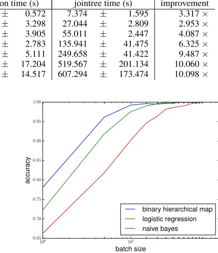
Route Classification.We report results on route classifi-cation in Figure 8. We consider two classes of routes from two datasets: (1) thecabspottingdataset (Taxi), and (2) a simulated dataset collected by querying Google Maps Di-rections API with source/destination pairs (Google).14 We took 215 = 32,768 and 212 = 4,096 routes from each dataset for training/testing. We took a map of size 5,374 edges and learned a binary hmap, as in Section 5; the SBN had737,928parameters. We trained two sets of SBN param-eters (using Laplace smoothing), one for each dataset, yield-ing a (structured) naive Bayes classifier (Choi, Tavabi, and Darwiche 2016).15 The Taxi dataset was collected in 2008, which predates the proliferation of GPS navigators. Hence, we view our Google vs. Taxi classifier as discriminating be-tween drivers with/without GPS navigation, or alternatively, Uber drivers (with) vs Taxi drivers (without). Figure 8 sum-marizes our results, where we compare against (1) an (un-structured) naive Bayes classifier (2) and a logistic regres-sion classifier. Both uses each edge as a binary feature (each edge is either present or absent). On thex-axis, we provide each classifier with a batch of routes of increasing size, from 1 to 60. Each batch of sizexis a set ofxroutes of the same type—the idea is that the one can better distinguish a driver as an Uber or a taxi driver, as more routes from the same driver are provided. As we give each classifier more routes from the same type of driver, we achieve higher accuracy (as expected), converging to 100% accuracy. Clearly, our SBN (using a binary hmap) is superior to logistic regression, which in turn is superior to naive Bayes.
7
Conclusion
In this paper, we proposed the first exact inference algo-rithm for structured Bayesian networks (SBNs), based on compiling SBNs to PSDDs. We highlighted the importance of vtrees for the purposes of inference and separately for learning. Next, we identified a tractable sub-class of SBNs based on binary hierarchical maps, for learning route distri-butions. We also proposed an algorithm to learn the struc-ture of binary hierarchical maps from data. Empirically, we showed that inference based on compilation can be an order-of-magnitude more efficient compared to jointree inference. In our experiments, we demonstrated the practical utility of our algorithms using route distributions learned from read-world GPS data. We showed that our inference algorithm can scale to much larger maps than those previously con-sidered, and that our learning algorithm can learn struc-tures with improved route-prediction performance. Finally, we demonstrated the utility of binary hierarchical maps for the purposes of route classification.
14
In particular, we initially took the map of size 5,202 from Ta-ble 1, and from thecabspottingdataset, we took all 172,265 routes strictly contained in the map. For each route, we took the source, destination, day-of-week and time-of-day, which we used to request a corresponding route from Google Maps.
15
If a train/test route is invalid (visits the same region twice), then it has probability zero in the SBN. In this case, we segment the route into multiple valid routes, as in Footnote 6, for training. For testing, we observe each route segment as a feature in the structured naive Bayes classifier.
Acknowledgments We thank John Stucky and Yaacov Tarko for comments and discussions on this paper. This work has been partially supported by NSF grant #IIS-1514253, ONR grant #N00014-18-1-2561 and DARPA XAI grant #N66001-17-2-4032.
A
Proof of Theorem 1
We provide a construction of the joint PSDD in this section. For a given region, we refer to itsexternaledges as those edges that have one endpoint inside the region and the other endpoint outside the region. External edges are the edges that are used to enter and exit a region. Further, a path is simpleif it does not visit the same node twice. We say that a path ishierarchically simpleif it does not visit the same region twice, in the hmap. In an SBN of a binary hmap, all paths must be hierarchically simple; otherwise, they have probability zero (Choi, Shen, and Darwiche 2017).
Consider a leaf nodecin a binary hmap. We want the PS-DDs representing routes inside this region. Under the hier-archical simple-path assumption, at most two external edges will be used—we cannot visit the same region twice. At the most, we can enter and exit a region.
When exactly two external edges e1 and e2 are used,
we want a PSDD over all simple paths that connect to bothe1 ande2 in the region c. We refer to this PSDD as non-terminalc(e1, e2), because all paths must pass through
the region c. When exactly one external edge e is used, we want a PSDD over all simple paths that start at edge
e and then end inside regionc. We refer to this PSDD as
terminalc(e),because all paths terminate in regionc. Finally,
if no external edge is used, we want a PSDD over all sim-ple paths strictly contained inside the region. We refer to this PSDD asinternalc. In PSDDsterminalc(e)and PSDDs
non-terminalc(e1, e2)that connect to the same endpoint
in-side the region, we allow for an empty path inin-side the region. Further, we assume that all PSDDs non-terminalc(e1, e2), terminalc(e), andinternalc have a bounded size. This can be ensured by using a binary hmap that is deep enough to have small enough regions. In our experiments, we used theGRAPHILLIONpackage16to compile regions into ZDDs,
which are then converted to SDDs.
Consider an internal nodecin a binary hmap, which has a left child regionland a right child regionr. Each internal nodecis itself a binary hmap, rooted atc. It represents a map consisting of all nodes and edges inside the corresponding binary hmap. As we did previously, we will construct PS-DDsnon-terminalc(e1, e2),terminalc(e)andinternalcover
the different types of routes implied by the selected external edges. These PSDDs can be specified using the PSDDs of its left and right child sub-regions.
Suppose we have external edgese1, . . . , en,and the edges m1, . . . , mk that cross between the left and right
sub-regions. Letemptyc denote the PSDD forc containing no routes (all edges must be set to false). Consider the PSDD
internalc. An internal route is either (1) strictly contained in the left region, (2) strictly contained in the right region,
16
or (3) it crosses the two regions using exactly one edgemi.
Thus, the corresponding SDD has the elements:
internall,emptyr emptyl,internalr
terminall(m1),terminalr(m1)
.. .
terminall(mk),terminalr(mk)
By the hierarchical simple-path assumption, the path be-tween the left and right regions must consist of a single edge. Consider the PSDDs terminalc(e). Suppose that e con-nects to a node in the left child region (the case for the right child is symmetric). There are two cases: (1) the path stays in the left, or (2) the path crosses into the right using one edgemi. This PSDD has an SDD with the elements:
terminall(e),emptyr
non-terminall(e, m1),terminalr(m1)
.. .
non-terminall(e, mk),terminalr(mk)
Consider the PSDDsnon-terminalc(e1, e2). Suppose thate1
connects to the left child region and thate2connects to the
right child region (the reverse case is symmetric). Here, the path must cross from the left to the right using one edgemi.
This PSDD has an SDD with the elements:
non-terminall(e1, m1),non-terminalr(m1, e2)
.. .
non-terminall(e1, mk),non-terminalr(mk, e2)
Ife1 ande2 both connect to the same region, say the left
one, then the path must stay inside the left region. We have an SDD with a single element:
non-terminall(e1, e2),emptyr.
To count the total size of the joint PSDD, we count the num-ber of PSDD nodes that we constructed, and also count the size of each node (number of elements). Moreover, we do not count elements with a false sub in our PSDD, which are not needed to represent the distribution. First, for a leaf node in the binary hmap, ifnis the number of its external edges, then we haveO(n2)distinct PSDDs, each having a bounded
sizem.If there aretnodes in the binary hmap, then there areO(t)leaf nodes. Hence, the total size of the leaf PSDDs isO(t·n2·m).Second, for an internal node in the binary
hmap, ifnis the number of its external edges, then we have
O(n2)PSDD nodes. Ifkis the number of edges that cross
between the left and right sub-regions, then the PSDD node hasO(k)elements. Thus, the number of PSDD nodes for internal nodes in the binary hmap isO(t·n2)and their
ag-gregate size isO(t·n2·k). Thus the total size of the joint
PSDD isO(t·n2·m+t·n2·k).
References
Boutilier, C.; Friedman, N.; Goldszmidt, M.; and Koller, D. 1996. Context-specific independence in Bayesian networks.
InProceedings of the Twelfth Annual Conference on Uncer-tainty in Artificial Intelligence (UAI), 115–123.
Choi, A., and Darwiche, A. 2013. Dynamic minimization of sentential decision diagrams. InProceedings of the 27th Conference on Artificial Intelligence (AAAI).
Choi, A.; Shen, Y.; and Darwiche, A. 2017. Tractability in structured probability spaces. InNIPS, 3480–3488.
Choi, A.; Tavabi, N.; and Darwiche, A. 2016. Structured features in naive Bayes classification. InProceedings of the 30th AAAI Conference on Artificial Intelligence (AAAI). Darwiche, A. 2011. SDD: A new canonical representation of propositional knowledge bases. InProceedings of IJCAI, 819–826.
Groves, W.; Nunes, E.; and Gini, M. L. 2014. A frame-work for predicting trajectories using global and local in-formation. InProceedings of the 11th ACM Conference on Computing Frontiers, 1–10.
Kisa, D.; Van den Broeck, G.; Choi, A.; and Darwiche, A. 2014. Probabilistic sentential decision diagrams. In Pro-ceedings of the 14th International Conference on Principles of Knowledge Representation and Reasoning (KR).
Krumm, J. 2008. A Markov model for driver turn prediction. Technical report, SAE Technical Paper.
Larkin, D., and Dechter, R. 2003. Bayesian inference in the presence of determinism. InAISTATS.
Liang, Y.; Bekker, J.; and Van den Broeck, G. 2017. Learn-ing the structure of probabilistic sentential decision dia-grams. In Proceedings of the 33rd Conference on Uncer-tainty in Artificial Intelligence (UAI).
Murphy, K. P. 2012. Machine Learning: A Probabilistic Perspective. MIT Press.
Oztok, U.; Choi, A.; and Darwiche, A. 2016. Solv-ing P PP P-complete problems using knowledge compila-tion. In Proceedings of the 15th International Conference on Principles of Knowledge Representation and Reasoning (KR), 94–103.
Piorkowski, M.; Sarafijanovoc-Djukic, N.; and Gross-glauser, M. 2009. A Parsimonious Model of Mobile Par-titioned Networks with Clustering. In The First Interna-tional Conference on COMmunication Systems and NET-workS (COMSNETS).
Shen, Y.; Choi, A.; and Darwiche, A. 2016. Tractable operations for arithmetic circuits of probabilistic models. In Advances in Neural Information Processing Systems 29 (NIPS), 3936–3944.
Shen, Y.; Choi, A.; and Darwiche, A. 2017. A tractable probabilistic model for subset selection. InProceedings of the 33rd Conference on Uncertainty in Artificial Intelligence (UAI).
Shen, Y.; Choi, A.; and Darwiche, A. 2018. Conditional PSDDs: Modeling and learning with modular knowledge. In Proceedings of the 32nd AAAI Conference on Artificial Intelligence (AAAI), 6433–6442.