Modelling Space-time Propagation of Climate Sensitive Variation in the Indus River Flow

(1)

Modelling Space-time Propagation of Climate

Sensitive Variation in the Indus River Flow

Syed Ahmad Hassan

1



1

Department of Mathematics, University of Karachi, Karachi-75270, Pakistan

Abstract: The linear and nonlinear analyses of the impacts of local climatic parameters on Indus River flows as discussed in [1] and [2] gives provision to investigate the influential role of the regional climatic parameters. For this purpose this paper simulates the Indus River flow network using exponentially distributed river network (SRN) feed by employs synthetically generated local temperature and rainfall dependent runoffs. The local temperature and rainfall is generated using the stochastic, autoregressive and Poisson process methods respectively. To explore the influential role, the sensitivity analyses are performed by changing the local climatic parameter values. This demonstrates the existence of relation between the variability of temperature and rainfall on the river flow in the form of linear and nonlinear information and its propagation along the network. In the mean 10daily flow (TDF) propagation the dominant precipitation characteristic is linear. It is to be saying that the temperature variations make some way of only nonlinear behaviour in the TDF propagation. Accordingly, it explores the impact of local climatic parameters on the river flow and its propagation in the form of linear and nonlinear information.

Keywords: Indus River, Local Climate, Propagation, River network

1 Introduction

Pakistan suffered a cluster of torrential rain events, causing the worst flooding in 100 years [3]. About 1700 people perished and 1.8 million homes were lost, rendering 20 million people homeless, with an economic loss estimated to be more than $40 billion U.S. [4]. The arena of problems like correct assessment, proper storage, reliable control and judicious distribution of existing water masses among various provinces/regions within Pakistan is properly encompassed by technical research and mathematical modelling. Keeping in view the preliminary local climatic analyses as presented in Hassan and Ansari (2015) and linear and nonlinear analyses performed in Hassan and Ansari, (2010), and Hassan (2011) [1-5], this paper assess the impact of climatic parameters (Temperature & Rainfall) on mean 10daily river flow (TDF) along the Indus River.

A detailed knowledge of river geomorphology, river dynamics, their branching process and flood routing is fundamental for the analyses required for long-term flood forecasting and management. Study of river networks is, thus, very essential for this purpose. The setback with conventional statistical/probabilistic or stochastic networks is that they ignore the nonlinearity inherent in the problem. The river system network consists of links and nodes classically defined by work on tributaries and the interaction of main stream including junction hydraulics and mixing their work on the structure [6-9]. However, from mid-1980’s, tributaries and the

(2)

Modelling Space-time Propagation of Climate Sensitive Variation in the Indus River Flow

construct an exponentially distributed river network (SRN) for the simulation of Indus River. This SRN utilizes synthetically generated local temperature and rainfall (details discussed in next sections) to replicate the Indus River flow. To check the existence and propagations of linear and nonlinear information (components) in this river flow, the sensitivity analyses will performed by changing the average climatic parameter values. These analyses will demonstrate any possibility of existence of a relation between the variability of local climatic parameters and the river flow in the form of linear and nonlinear information and its propagation along the network. Moreover, the outcomes tell us about the impact of local climatic parameters on the river flow and its propagation.

The sec. 2.1 will perform simulation of the Indus River flow and comparison between the behaviours of real and simulated river flow propagation Patterns along the Network. Sec. 3 deals with results and discussion related to Influence of Climatic factors on River Flow Propagation and finally sec. 4 conclude the paper

2. Materials and Methods

2.1 Simulated Modelling of the River

Network

For simulation of River network, construct a SRN, and customise it to match the Indus River network

(Table 1). It is assumed that the catchment areas and the inter-catchment distances of the network are exponentially distributed (Table 2). This networked has a main stream starting as an outsourcing of a big main catchment and other catchments are linked in the downstream. It is further assumed that the main catchment area is about 75% (to simulate Upper Indus Basin above Tarbela), and the sum of the other catchments are being 25% (catchments of the Indus River below Tarbela) of the total of all catchment areas (Fig. 1). The generated inter-catchment distances of SRN only considers catchment-1, 2, 3, 4, 6, 7 and 9 because they are in close relation to that of Indus River network (Table 1 & 2). The altitudinal range of each catchment is obtained from linearly approximated general hypsometric curve [18] of the UIB region (Fig. 2, Table 3). To feed these catchments, the daily sum of precipitation is synthetically generated by Poisson process and the daily mean temperature (MDT) is generated by using autoregressive AR(2) model [19]. The mean annual temperature decreases with increasing altitude values (Table 4). To simulate these variations, the approximately estimated temperature lapse rate value is about 0.0065 oC m-1 (Table 4). To setup the elevation dependent annual sum of precipitation lapse rate, break the 4 to 7500m altitude range in to three ranges 4500m, 5001250m and 12507500m.

Table 1 Reference station related distances from lower three stations all their upstream stations along Indus River. All distances are in canal km (Source: Irrigation and power department, Government of the Punjab, Lahore)

Distances from  to

 Sukkur Guddu Taunsa Chasma Kalabagh Tarbela

Kotri 479.57 690.39 991.33 1235.94 1334.11 1535.27

Sukkur 0.00 209.21 511.76 756.37 854.54 1055.70

(3)

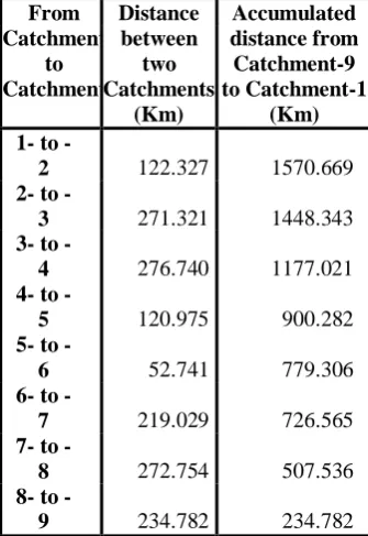
Table 2 Detail of exponential distributed all inter-catchment distances and accumulated inter-catchments distances from catchment-9 to catchment-1

From Catchment

to Catchment

Distance between

two Catchments

(Km)

Accumulated distance from Catchment-9 to Catchment-1

(Km) 1 to

-2 122.327 1570.669

2 to

-3 271.321 1448.343

3 to

-4 276.740 1177.021

4 to

-5 120.975 900.282

5 to

-6 52.741 779.306

6 to

-7 219.029 726.565

7 to

-8 272.754 507.536

8 to

-9 234.782 234.782

Table 3 Detail of all catchments altitudinal ranges with its minimum and maximum altitudinal values

No. Area

(km2)

Altitude range

(km)

Altitude range with in catchment (m) Minimum Maximum 1 170000.00 7.0 500 7500.00

2 7743.62 0.319 400 718.855

3 6312.32 0.260 350 609.919

4 10916.47 0.450 300 749.502

5 9509.10 0.392 275 666.551

6 5954.84 0.245 250 495.199

7 257.51 0.011 225 235.603

8 10161.83 0.418 150 568.428

9 5810.96 0.239 100 339.275

Table 4 Temperature lapse rates based in Annual mean temperature during 1977-97of available cites data out of these approximately 0.0065 oC m-1 lapse rate is selected

City Altitude

(m)

Annual Mean Temp. (C)

Name of the two cities lapse rates (LP)

Lapse rate (LP) between two

cities (C m-1)

Skardu 2181

11.83690

5 Skardu - Gilgit -0.0054

Gilgit 1459

15.75912

7 Gilgit - Kakul -0.0039

Kakul 1309 16.35 Kakul - Karachi -0.0079

Karachi 4 26.66 Average of

above three LP -0.0058

Overall LP (Skardu –

Karachi) -0.0068

Average of

(4)

Fig. 1 Structure of the exponentially distributed river network (EDRN) to simulate the Indus River.

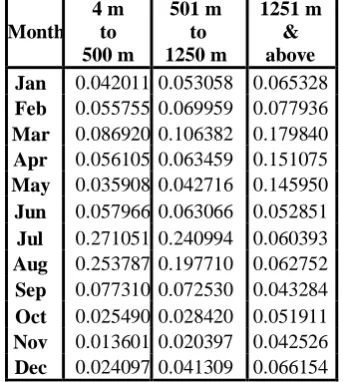
The lapse rates for three ranges are 2.386, 0.8, and 0.261 mm m-1 respectively estimated from available local data (Fig. 3). Usually, there are two precipitation systems, the monsoon (summer), and the western disturbance (winter and spring) affect different altitude ranges annual SMP patterns in Pakistan [20]. Consequently, It is further assumed the three different patterns of the annual SMP (relative rates) for the above mentioned three altitude ranges (Table 5 & Fig. 4).

Table 5Sum of monthly precipitation (in percentage) according to the annual sum of rainfall of the each altitude range

Month 4 m

to 500 m

501 m to 1250 m

1251 m & above Jan 0.042011 0.053058 0.065328

Feb 0.055755 0.069959 0.077936

Mar 0.086920 0.106382 0.179840

Apr 0.056105 0.063459 0.151075

May 0.035908 0.042716 0.145950

Jun 0.057966 0.063066 0.052851

Jul 0.271051 0.240994 0.060393

Aug 0.253787 0.197710 0.062752

Sep 0.077310 0.072530 0.043284

2.2 Catchments’ Runoff Generation

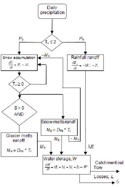
To feed the modelled SRN, synthetically generated precipitation and temperature dependant snow-glacier melt runoffs are utilized to produce the daily outflow of each nine catchments with following model (Fig. 5):

 

rW L M M kR dt dW

c G S

R    

 (1.2)

where W is the catchment water production,

kR

_R, MS

and MG are the rainfall, snow melt glacier melt

runoffs respectively. Whereas Lc (section 2.2.2) and

rW is the portion of storage to form outflow ( = 1 for linear). The schematic diagram of Fig. 5 provides an understanding of the working of the module apply Linearly approximated general hypsometric curve of the Upper

Indus Basin (UIB)

Linear approximation y = 27.269x + 2290.1 with R2

= 0.8485

0 1000 2000 3000 4000 5000 6000 7000 8000 9000 10000

0 50 100 150 200

Area (km ^2)

H

e

ig

h

t

(m

)

Height Linear (Height)

0 1000 2000 3000 4000 5000 6000 7000 0

200 400 600 800 1000 1200 1400 1600 1800 2000

Altitude (m)

P

re

c

ip

ita

tio

n

(

m

)

According to historical data & previous studies Linear by parts approximation for simulation

1 2 3 4 5 6 7 8 9 10 11 12

0 0.05 0.1 0.15 0.2 0.25

Month (January- to- December)

M

o

n

th

ly

p

re

c

ip

ita

tio

n

f

ra

c

tio

n

in

%

o

f

a

n

u

a

l s

u

m

o

f

p

re

c

ip

ita

tio

n Alt. = 1250 m & above 500 m <= Alt. < 1250 m 4 m <= Alt. < 500

Fig. 2 linear approximation of the general hypsometric for the upper Indus basin (UIB) defined by Hewitt, (1993) (Hewitt, 1993) above Tarbela Dam showing approximate altitudes of precipitation zones. The curve is derived from 2000ft contour intervals on map sheet of the area at scale of 1:250,000. The linear equation is y = 27.269 x + 2290.1, where x is the area in km2 and y its relative height in km, with residual sum of square R 2

= 0.8485. This linear approximation is used to set the altitudes with in each catchment of EDRN

Fig. 3 Annual sum of precipitation (1977–97) with respect to altitude provide precipitation lapse rate according to the historical data and previous studies (– – – –), we linearly approximate these lapse rate by parts () in to three regions

(5)

(i) If the daily temperature  2oC so, the falling precipitation will be snow otherwise it is rainfall. Moreover, new snowfall is added to snowpack, glacier region or plain ground, as water equivalent. (ii) Rainfall runoff (liquid accumulates) promptly contributes to river flows whereas, the snowmelt runoff provides a delayed base flow the catchment runoff.

(iii) If the daily temperature increases from the threshold Th = 0oC, it is assumed that snowmelts is at

the rate of 1.5 mm oC-1day-1. when all the liquid and snowpack are depleted in the glacier region the ice melt occurs at the rate of 4 mm oC-1 day-1 [21].

Temperature generation, The annual patterns of mean monthly temperature (MMT) variations of all cities are approximately the same. The generation of MDT follows autoregressive AR(2) model added (superimposed) on the linear interpolated MDT value from historical annual pattern of MMT, and normally distributed noise and defined as :

Tt= dt + b1Tt1 +b2 Tt2 + et (1.3)

Where Tt is the generated MDT at time t, dt is the

linear interpolated MDT, b1 and b2 are the

coefficients of the AR(2) terms Tt1 and Tt2

respectively and et is the normally distributed random

noise with mean 0 and variance 1. This method may be capable in replicating the actual MDT and with help of temperature lapse rate (as defined above) they generates the MDT of all the catchments.

The daily outflow module of the catchments,

Precipitation is the major source to produce runoff in the daily outflow module of the catchments (Fig. 5). The precipitations of these catchments are generated by marked Poisson process [22]. The daily generated precipitation events are summed up and their respective depth to the daily sum of precipitation in mm/day. If MDT value, is Tt < 2 C the daily

precipitations P will become snowfall PS and if Tt 2

C then it will considered as PR the rainfall. The daily

rainfall PR spikes transform in to rainfall runoff RR

[22] using:

R R

R

_kR

_P

dt

dR

_

_



_

(1.6)

where



kR

_R is the decay recession effect in RR, and

 is the factor to set the decay recession flow and k

represents the coefficient of recession flow. Moreover, the daily snowfall accumulates as liquid equivalents on the old accumulated snow, glacier, or ground as follows:

S

M

P

dt

dS

_

_

(1.7)

where dS/dt is the rate of variation in the snow

snowmelt runoff respectively (depends on degree-day factor DFS). When Tt 0C then MS = Tt DFS and if

snow cover vanish on the glaciated area then glacier melt starts with the degree-day factor of glacier DFG

as, MG = TtDFG, where MG is the daily glacier melt

runoff value.

Fig. 5 Schematic diagram of catchment daily outflow module based on rainfall runoff, snow and glacier melt runoffs components respectively

2.2.2 The generalized losses

This simulation method considers two types of water losses, evaporation and seepage, during runoff generation and the propagation of river flow along the SRN respectively.

Evaporation in the catchment, It is assumed that the minimum to maximum evaporation Lct in the

catchment are 0 to 5 mm/day respectively and are linearly dependant on the MDT (Tt ) of the catchment

as:

Lct= 

  

 

 2)( 2) (

5

t tamx

T

T (1.8) where Lct is the straight line (linear) relation between

(2C, 0 mm) and (TtamxC, 5mm) coordinates. Where

Ttamx is the annual maximum MDT of the catchments.

(6)

the evaporation assume the following relation of Lctto

the net daily loss due to evaporation Lc (mm/day).

Lc=Lct 

  

 



amx

P P

1 (1.9)

where Pamx is the annual maximum daily

precipitation, and P is the daily precipitation. Substituting the values of equation (1.6), MS, MG, and

(1.9)in the water storage equation (1.2) then get the outflow of the catchment Q = r W. The same procedure applies to all nine SRN catchments to generate the respective daily out flows.

To consider base flow from catchment-1 due to the ground water contribution of the deep snowpack and glacier areas [23-24] it is assumed that a fixed value of Qb= 250 m3/s is generated from the catchment

continuously. The out flow represented as 1

i

Q

= Q1 +

Qb and from the other catchments are

Q

_ic = Qc,

where c is the catchment number and i is the day.

Seepage along the River, The seepage losses is assumed to be about 3% per 10 miles or 0.186% km1 [25]. The final flow Ff and the initial flow Fi are

related as:

)

00186

.

0

1 (

_t

i

f

F

d

F





(1.10) where dt is the distance (km) travelled by water mass

along the main stream.

Diffusion behaviour is introduced by multiplying the seven (7) days moving average river flow by lognormal weighted noise. To make real daily variations in the diffused (smooth) river flow add some lognormal distributed noise i as

2.4 River flow propagation method

The daily outflow of each catchment needed some diffusive and velocity shifting behaviour to simulate the travelling of water mass along the main stream. Diffusion behaviour is introduced by multiplying the seven (7) days moving averaged river flow by lognormal weighted noise wj. To make some real

daily variations in the diffused (smooth) river flow add some lognormal noise i as follows:

i j j

N j i N

i

Q

w

Q













 

3

; where

Q

iNis the

diffused ith river flow of the Nth catchment. The velocity shifting behaviour is introduced by some negative lag ( e positions) shifting of the river flow values . The ith river flow

Q

iN shifted to the lag = e

as

Q

_ic_,_d(where i represents the ith daily flow of the catchment-c after the dth catchment represent the location of the river flow record in SRN) as:

b i

i

Q

1_,₁



1



where

Q

_i1_,₁is the ith daily flow of the catchment-1, and Qb is the base. The remaining all

flow records location after each catchment-2 to 9 in SRN is represented as:

i j

j c

c j c e i c

i c

d

i

Q

w

Q











 



  

3

3 1

1 }, )] ( {[

,

*

; where

c d i

Q

_, is the ith river flow record after location

d and c is the catchment number (c = 2, 3, 4, 5, 6, 7, 8, 9). After generating daily river flows of each location of the SRN, convert all of them to the

10daily river flows (TDF)

Q

_Tic_,_d for the further LM and NLM analysis.

3.1 Comparison between the behaviours of

real and simulated river flow propagation Patterns

To calibrate TDF of the main stream generated by catchment-1compare with the TDF of Tarbela station. This shows a better simulation of the 10daily out flow at Tarbela station. The next step will simulate the behaviour of cross correlation (CC) and normalized cross mutual information (MI) of the Indus River and the generated TDFs’.

The Fig. 6a shows the CC analysis between catchment-9 (last station of SRN) with itself and with all its upstream stations (catchment-7, 6, 4, 3, 2, & 1). It also represents proper simulation of the real LP curve as mention in Fig. 4.3a of Hassan (2011) however, a relatively slower roll off of simulated LP curve found. This behaviour happened because the simulation utilized limited number of dominating parameters instead of large number of actual parameters involved in the real river flow. Repeat the same procedure for catchment-7 and catchment-4 (Fig. 6b & c) and skip the catchment-6 because it does not match the contours of the real LP curves from third last station (Guddu). The above simulation showed by using CC analysis of TDF it is clear that the contours of the real LP curves as mention in Fig. 4.3a of Hassan & Ansari (2011) and the simulated LP curves (Figs. 6a-c) are similar.

(7)

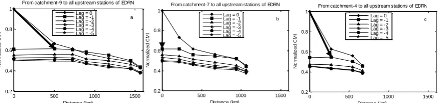
Fig. 4.4a of [5]. The NP curves from the last three reference stations in real network and from catchment-9, 7, & 4 in the SRN simulated NP curves are similar (Fig. 7a-c). To explore the impact of real local climatic variability in the river flow, the next

section analyses the variations in the propagation of linear and nonlinear information (LP and NP curves) under the climatic influence along the whole SRN network.

Fig. 6 Linear information propagation roll-off (LIPR) behaviour obtain from distance dependent CC analysis of the EDRN simulated Indus River (simulate the space-time cross-correlation analysis along the Indus River Fig. 4.3 of Hassan (2011)), from lower three stations separately with itself and with all their selected upstream stations of EDRN: (a) from catchment-9, (b) from catchment-7, and (c) from catchment-4

Fig. 7 Nonlinear information propagation roll-off (NLPR) behaviour obtain from distance dependent CMI analysis of the EDRN simulated Indus River (simulate the space-time cross-correlation analysis along the Indus River Fig. 4.4 of Hassan (2011)), from lower three stations separately with itself and with all their selected upstream stations of EDRN: (a) from catchment-9, (b) from catchment-7, and (c) from catchment-4

3: Results and Discussion

This section will show how temperature and rainfall variations influence the river flow and its propagation. To implement this idea analyse the changes in LP and NP curve (Fig.6 & 7) variations by introducing some changes in the normally simulated temperature and rainfall values.

Impact of rainfall variations, To observe linear influence in the river flow propagation introduce 10% and 20% increase in the simulated annual sum of rainfall (ASRF) values. The results shows some gradually raise (or slow roll-off) in the simulated CC value curves (Fig. 6a). The resultant LP curves (Figs. 8a & b) demonstrate increasing trends. This trend is retains for 30%, 40%, and 50% increase in ASRF.

Moreover, the 10% and 20% decrease in the ASRF values, CC and LP curves shows gradual quick roll-off for each change (Figs. 8c & 8d). This trend continues for 30%, 40%, and 50% decrease in ASRF values. These variations explore that the increasing rainfall may behave linearly in the river flow propagation along the network. To explore the nonlinear effect of rainfall the simulated NP curve (Fig. 7a) propagates only to the next station (catchment-7, lag = 1). However, 10% increase in ASRF makes NP curve (Fig. 9a) to prolong more and end at a longer distance (catchment-6) and at lower lag (lag = 2). Further development in MI and resultant NP curve variations are shown in Table-6.

0 500 1000 1500

0.3 0.4 0.5 0.6 0.7 0.8 0.9 1

Distance (km)

C

ro

s

C

o

rr

e

la

tio

n

From catchment-9 along all upstream stations of EDRN

Lag = 0 Lag = -1 Lag = -2 Lag = -3 Lag = -4 Lag = -5 a

0 500 1000 1500

0.3 0.4 0.5 0.6 0.7 0.8 0.9 1

Distance (km)

C

ro

s

c

o

rr

e

la

tio

n

Lag = 0 Lag = -1 Lag = -2 Lag = -3 Lag = -4 Lag = -5 b

0 500 1000 1500

0.3 0.4 0.5 0.6 0.7 0.8 0.9 1

Distance (km)

C

ro

s

c

o

rr

e

la

tio

n

Lag = 0 Lag = -1 Lag = -2 Lag = -3 Lag = -4 Lag = -5 d

0 500 1000 1500

0.2 0.4 0.6 0.8 1

Distance (km)

N

o

rm

a

liz

e

d

C

M

I

From catchment-9 to all upstream stations of EDRN

Lag = 0 Lag = -1 Lag = -2 Lag = -3 Lag = -4 Lag = -5

a

0 500 1000 1500

0.2 0.4 0.6 0.8 1

Distance (km)

N

o

rm

a

liz

e

d

C

M

I

b

0 500 1000 1500

0.2 0.4 0.6 0.8 1

Distance (km)

N

o

rm

a

liz

e

d

C

M

I

(8)

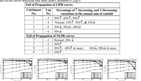
Table 6 Impact of percentage  Increasing or  Decreasing variations in the annual sum of rainfall on the LIPR and NLPR curves behaviour that starts from Catchment-9, Lag-0

Fall of Propagation of LIPR curves

Catchment No.

Lag No.

Percentage of  Increasing, and  Decreasing variations in the annual sum of rainfall

1 3 20%, 40%, 50%

1 4 Normal, 10%, 30%, & 10% 1 5 20%, 30% , 40%

2 4 50%

Fall of Propagation of NLPR curves

7 1 Normal, 20%  7 2 30%

6 1 20%, 40%& more; 10%, 30%& more 6 2 10%

Fig. 8 Variations in the LIPR curve (based on CC value curves behaviour of the MTDRF along the EDRN from catchment-9 with itself and with all its selected upstream stations) at four different deviations in the normally simulated ASRF values: (a) 10% increase, (b) 20% increase, (c) 10% decrease, and (d) 20% decrease

Fig. 9 Variation in the NLPR curve (based on NCMI value curves behaviour of the MTDRF along the EDRN from

catchment-9 with itself and with all its selected upstream stations) at four different deviations in the normally simulated ASRF values: (a) 10% increase, (b) 20% increase, (c) 10% decrease, and (d) 20% decrease

Impact of temperature variations, When AMT

values increases from +1 to +3C the CC value curves slightly loses their level and resultant LP curve shows slightly sharper roll-off, ending at same catchment-1 but at lower lag = 5 (Fig. 10a). Further +4 to +7 C increase in the AMT value the CC curves gradually increase their levels and resultant LP curve increases to their normally simulated contours ending at same catchment-1 and lag = 4 (Figs. 10b & 10c). A reduce to 1C in AMT value makes no significant change (Fig. 10d) in normally simulated CC and LP curve (Fig. 10a). A 2 C reduce in AMT value increases the levels of normally simulated CC values and the resulting LP curve (Fig. 10e) ending at higher lag = 3. More reduction in the AMT value will

+1C increase in AMT values makes no change in the normally simulated MI based NP curve (Fig. 11a) . Further +2C increase in AMT level makes NP curve (Fig. 11b) prolong to a larger distance ending at catchment-6 and lag = 2. Further development in the MI and resultant NP curve due to the increase and decrease AMT level is as shown in Table-7. In view of the AMT variation analysis there is no trend no dominant mechanism found in the linear behaviour (LP) of the river flow. However, The positive increment in the normally simulated ATM values make a short cyclic affect in the NP curve ending catchment and lag values from +1C to +6C. This cyclic affect indicates the influence of the positive temperature rise in nonlinear information

0 500 1000 1500

0.3 0.4 0.5 0.6 0.7 0.8 0.9 1 Distance (km) C ro s s c o rr e la tio n

From catch.-9 along EDRN w ith 10% increase of annual rainfall

0 500 1000 1500

0.3 0.4 0.5 0.6 0.7 0.8 0.9 1

Distance (km) C ro s s c o rr e la tio n

0 500 1000 1500

0.3 0.4 0.5 0.6 0.7 0.8 0.9 1

From catch.-9 along EDRN w ith 10% decrease of annual rainfall

Lag = 0 Lag = -1 Lag = -2 Lag = -3 Lag = -4 Lag = -5 c

0 500 1000 1500

0.3 0.4 0.5 0.6 0.7 0.8 0.9 1

0 500 1000 1500

0.4 0.5 0.6 0.7 0.8 0.9 1 Distance (km) N o rm a liz e d C M I

From catch.-9 along EDRN w ith 10% increase of annual rainfall Lag = 0 Lag = -1 Lag = -2 Lag = -3 Lag = -4 Lag = -5

a

0 500 1000 1500

0.4 0.5 0.6 0.7 0.8 0.9 1

Distance (km) N o rm a liz e d C M I

b

0 500 1000 1500

0.4 0.5 0.6 0.7 0.8 0.9 1

c

0 500 1000 1500

0.4 0.5 0.6 0.7 0.8 0.9 1

(9)

Fig. 10 Variations in the LIPR curve (based on CC value curves behaviour of the MTDRF along the EDRN from catchment-9 with itself and with all its selected upstream stations) at four different deviations in the normally simulated AMT values: (a) 1C increase, (b) 4C increase, (c) 5C increase, (d) 1C decrease, (e) 2C decrease, , (f) 5C decrease and (g) 7C decrease

Fig. 11 Variations in the NLPR curve (based on NCMI value curves behaviour of the MTDRF along the EDRN from catchment-9 with itself and with all its selected upstream stations) at four different deviations in the normally simulated AMT values: (a) 1C increase, (b) 2C increase, (c) 3C increase, (d) 1C decrease, (e) 2C decrease, and (f) 4C decrease

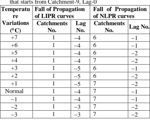
Table 7 Impact of C variations in the annual mean temperature on the LIPR and NLPR curves behaviour that starts from Catchment-9, Lag-0

Temperatu re Variations

(C)

Fall of Propagation of LIPR curves

Fall of Propagation of NLPR curves Catchments

No.

Lag No.

Catchments

No. Lag No.

+7 1 4 6 1

+6 1 4 6 1

+5 1 4 6 2

+4 1 4 7 2

+3 1 5 6 1

+2 1 5 6 2

+1 1 5 7 2

Normal 1 4 7 1

1 1 4 7 1

2 1 3 7 2

4 1 3 6 1

5 1 4 6 1

6 1 4 6 1

7 1 4 6 1

4 Conclusion

In this paper climatic variability analysis was performed for the simulated model of the Indus River network. The response of variability of the climatic parameter values in the simulated models was recorded. The results obtained from the simulated modelling analysis are very promising. They also strengthen the idea of linear and nonlinear characterisation of influential role of the local climatic parameters. It is may be found that the precipitation influences the TDF propagation in linear way. Moreover, a small impact of positive increase in the precipitation values exhibits nonlinear

0 500 1000 1500

From catch.-9 along EDRN w ith +1o_{C in annual mean Temp.}

0 500 1000 1500

0.3 0.4 0.5 0.6 0.7 0.8 0.9 1 Distance (km) C ro s s c o re la tio n

From catch.-9 along EDRN w ith +4oC in annual mean Temp.

0 500 1000 1500

0.3 0.4 0.5 0.6 0.7 0.8 0.9 1

Distance (km) C ro s s c o re la tio n

Lag = 0 Lag = -1 Lag = -2 Lag = -3 Lag = -4 Lag = -5 c

0 500 1000 1500

0.3 0.4 0.5 0.6 0.7 0.8 0.9 1

From catch.-9 along EDRN w ith -1oC in annual mean Temp.

0 500 1000 1500

From catch.-9 along EDRN w ith -2o_{C in annual mean Temp.}

Lag = 0 Lag = -1 Lag = -2 Lag = -3 Lag = -4 Lag = -5 e

0 500 1000 1500

0.3 0.4 0.5 0.6 0.7 0.8 0.9 1

Lag = 0 Lag = -1 Lag = -2 Lag = -3 Lag = -4 Lag = -5 f

0 500 1000 1500

0.3 0.4 0.5 0.6 0.7 0.8 0.9 1

From catch.-9 along EDRN w ith -7oC in annual mean Temp.

Lag = 0 Lag = -1 Lag = -2 Lag = -3 Lag = -4 Lag = -5 g

0 500 1000 1500

0.2 0.4 0.6 0.8 1 Distance (km) N o rm a liz e d C M I

From catch.-9 along EDRN w ith +1oC in annual mean Temp. Lag = 0 Lag = -1 Lag = -2 Lag = -3 Lag = -4 Lag = -5

a

0 500 1000 1500

0.2 0.4 0.6 0.8 1

From catch.-9 along EDRN w ith +2oC in annual mean Temp.

b

0 500 1000 1500

0.2 0.4 0.6 0.8 1

c

0 500 1000 1500

0.2 0.4 0.6 0.8 1

d

0 500 1000 1500

0.2 0.4 0.6 0.8 1

From catch.-9 along EDRN w ith -2oCin annual mean Temp.

e

0 500 1000 1500

0.4 0.5 0.6 0.7 0.8 0.9 1

(10)

the TDF propagation the dominant precipitation characteristic is linear. Moreover, it may be explore that the temperature variations make some way of nonlinear behaviour in the TDF propagation.

5 Reference

1. Hassan SA, Ansari MR. Nonlinear analysis of seasonality and stochasticity of the Indus River. Hydrological Sciences Journal–Journal des Sciences Hydrologiques. 2010 Mar 29;55(2):250-65.

2. Hassan SA, Ansari MR. Hydro-climatic aspects of Indus River flow propagation. Arabian Journal of Geosciences. 2015 Dec 1;8(12):10977-82.

3. Lau WK, Kim KM. The 2010 Pakistan flood and Russian heat wave: Teleconnection of hydrometeorological extremes. Journal of Hydrometeorology. 2012 Feb;13(1):392-403.

4. WMO, Weather extremes in a changing climate: Hindsight on foresight. WMO-No. 1075, 2011:17 pp.

5. Hassan, S. A., Ph.D. Thesis: River flow modelling in view of climatic variability and management of floods in Pakistan’s ecology, University of Karachi, Pakistan (Part of research work done in DukeUniversity, USA) 2011.

6. Horton RE. Erosional development of streams and their drainage basins; hydrophysical approach to quantitative morphology. Geological society of America bulletin. 1945 Mar 1;56(3):275-370.

7. Krumbein WC. Flood deposits of Arroyo Seco, Los Angeles County, California. Bulletin of the Geological Society of America. 1942 Sep 1;53(9):1355-402.

8. Lyell C, Deshayes GP. Principles of geology: being an attempt to explain the former changes of the earth's surface, by reference to causes now in operation. J. Murray; 1830.

9. Shreve RL. Infinite topologically random channel networks. The Journal of Geology. 1967 Mar 1;75(2):178-86.

10. Best JL. Sediment transport and bed morphology at river channel confluences. Sedimentology. 1988 Jan 1;35(3):481-98.

11. Rodriguez-Iturbe I, Rinaldo A. Fractal river basins: chance and self-organization. Cambridge University Press; 2001 Aug 27.

12. Bigelow PE, Benda LE, Miller DJ, Burnett KM. On debris flows, river networks, and the spatial structure of channel morphology. Forest Science. 2007 Apr 1;53(2):220-38.

13. Binnie SA, Phillips WM, Summerfield MA, Fifield LK. Sediment mixing and basin-wide cosmogenic nuclide

analysis in rapidly eroding mountainous environments. Quaternary Geochronology. 2006 Feb 1;1(1):4-14.

14. Gasparini NM, Tucker GE, Bras RL. Downstream fining through selective particle sorting in an equilibrium drainage network. Geology. 1999 Dec 1;27(12):1079-82.

15. Sugiura A, Fujioka S, Nabesaka S, Sayama T, Iwami Y, Fukami K, Tanaka S, Takeuchi K. Challenges on modelling a large river basin with scarce data: A case study of the Indus upper catchment. Journal of Hydrology and Environment Research. 2014;2(1):59-64.

16. Antico A, Schlotthauer G, Torres ME. Analysis of hydroclimatic variability and trends using a novel empirical mode decomposition: application to the Paraná River Basin. Journal of Geophysical Research: Atmospheres. 2014 Feb 16;119(3):1218-33.

17. Ali S, Li D, Congbin F, Khan F. Twenty first century climatic and hydrological changes over Upper Indus Basin of Himalayan region of Pakistan. Environmental Research Letters. 2015 Jan 13;10(1):014007.

18. Hewitt K. Altitudinal organization of Karakoram geomorphic processes and depositional environments. InHimalaya to the sea 2002 Sep 26 (pp. 118-133). Routledge.

19. Box GE, Jenkins GM, Reinsel GC, Ljung GM. Time series analysis: forecasting and control. John Wiley & Sons; 2015 May 29.

20. Archer DR, Fowler HJ. Spatial and temporal variations in precipitation in the Upper Indus Basin, global teleconnections and hydrological implications. Hydrology and Earth System Sciences Discussions. 2004;8(1):47-61.

21. Kuchment LS, Gelfan AN. The determination of the snowmelt rate and the meltwater outflow from a snowpack for modelling river runoff generation. Journal of Hydrology. 1996 May 1;179(1-4):23-36.

22. Laio F, Porporato A, Ridolfi L, Rodriguez-Iturbe I. Plants in water-controlled ecosystems: active role in hydrologic processes and response to water stress: II. Probabilistic soil moisture dynamics. Advances in Water Resources. 2001 Jul 1;24(7):707-23.

23. Griffiths GA, Clausen B. Streamflow recession in basins with multiple water storages. Journal of Hydrology. 1997 Mar 1;190(1-2):60-74.

24. Tallaksen LM. A review of baseflow recession analysis. Journal of hydrology. 1995 Feb 1;165(1-4):349-70.