Journal of Machine Learning Research 18 (2017) 1-57 Submitted 8/14; Revised 7/16; Published 3/17
Spectral Clustering Based on Local PCA
Ery Arias-Castro [email protected]
Department of Mathematics University of California, San Diego La Jolla, CA 92093, USA
Gilad Lerman [email protected]
Department of Mathematics
University of Minnesota, Twin Cities Minneapolis, MN 55455, USA
Teng Zhang [email protected]
Department of Mathematics University of Central Florida Orlando, FL 32816, USA
Editor:Mikhail Belkin
Abstract
We propose a spectral clustering method based on local principal components analysis (PCA). After performing local PCA in selected neighborhoods, the algorithm builds a nearest neighbor graph weighted according to a discrepancy between the principal sub-spaces in the neighborhoods, and then applies spectral clustering. As opposed to standard spectral methods based solely on pairwise distances between points, our algorithm is able to resolve intersections. We establish theoretical guarantees for simpler variants within a prototypical mathematical framework for multi-manifold clustering, and evaluate our algorithm on various simulated data sets.
Keywords: multi-manifold clustering, spectral clustering, local principal component analysis, intersecting clusters
1. Introduction
The task of multi-manifold clustering, where the data are assumed to be located near surfaces embedded in Euclidean space, is relevant in a variety of applications. In cosmology, it arises as the extraction of galaxy clusters in the form of filaments (curves) and walls (surfaces) (Valdarnini, 2001; Mart´ınez and Saar, 2002); in motion segmentation, moving objects tracked along different views form affine or algebraic surfaces (Ma et al., 2008; Fu et al., 2005; Vidal and Ma, 2006; Chen et al., 2009); this is also true in face recognition, in the context of images of faces in fixed pose under varying illumination conditions (Ho et al., 2003; Basri and Jacobs, 2003; Epstein et al., 1995).
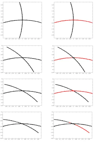
Figure 1: Two rectangular clusters intersecting at right angle. Left: the original data. Center: a typical output of the standard spectral clustering method of Ng et al. (2002), which is generally unable to resolve intersections. Right: a typical output of our method.
Spectral methods (Luxburg, 2007) are particularly suited for nonparametric settings, where the underlying clusters are usually far from convex, making standard methods like K-means irrelevant. However, a drawback of standard spectral approaches such as the well-known variant of Ng, Jordan, and Weiss (2002) is their inability to separate intersecting clusters. Indeed, consider the simplest situation where two straight clusters intersect at right angle, pictured in Figure 1 below. The algorithm of Ng et al. (2002) is based on pairwise affinities that are decreasing in the distances between data points, making it insensitive to smoothness and, therefore, intersections. And indeed, this algorithm typically fails to separate intersecting clusters, even in the easiest setting of Figure 1.
As argued in (Agarwal et al., 2005, 2006; Shashua et al., 2006), a multiway affinity is needed to capture complex structure in data (here, smoothness) beyond proximity at-tributes. For example, Chen and Lerman (2009a) use a flatness affinity in the context of
hybrid linear modeling, where the surfaces are assumed to be affine subspaces, and
sub-sequently extended to algebraic surfaces via the ‘kernel trick’ (Chen, Atev, and Lerman, 2009). Moving beyond parametric models, Arias-Castro, Chen, and Lerman (2011) intro-duce a localized measure of flatness.
Continuing this line of work, we suggest a spectral clustering method based on the esti-mation of the local linear structure (tangent bundle) via local principal component analysis (PCA). The idea of using local PCA combined with spectral clustering has precedents in the literature. In particular, our method is inspired by the work of Goldberg, Zhu, Singh, Xu, and Nowak (2009), where the authors develop a spectral clustering method within a semi-supervised learning framework. This approach is in the zeitgeist. While writing this paper, we became aware of two concurrent publications, by Wang, Jiang, Wu, and Zhou (2011) and by Gong, Zhao, and Medioni (2012), both proposing approaches very similar to ours.1 We also mention the multiscale, spectral-flavored algorithm of Kushnir, Galun, and Brandt (2006), which is also based on local PCA. We comment on these spectral methods
Spectral Clustering Based on Local PCA
in more detail later on. In fact, an early proposal also based on local PCA appears in the literature on subspace clustering (Fan et al., 2006)—although the need for localization is perhaps less intuitive in this setting.
The basic proposition of local PCA combined with spectral clustering has two main stages. The first one forms an affinity between a pair of data points that takes into account both their Euclidean distance and a measure of discrepancy between their tangent spaces. Each tangent space is estimated by PCA in a local neighborhood around each point. The second stage applies standard spectral clustering with this affinity. As a reality check, this relatively simple algorithm succeeds at separating the straight clusters in Figure 1. We tested our algorithm in more elaborate settings, some of them described in Section 4.
Other methods with a spectral component include those of Polito and Perona (2001) and Goh and Vidal (2007), which (roughly speaking) embed the points by a variant of LLE (Saul and Roweis, 2003) and then group the points by K-means clustering. There is also the method of Elhamifar and Vidal (2011), which chooses the neighborhood of each point by computing a sparse linear combination of the remaining points followed by an application of the spectral graph partitioning algorithm of Ng et al. (2002). Note that these methods work under the assumption that the surfaces do not intersect.
Besides spectral-type approaches to multi-manifold clustering, other methods appear in the literature. Among these, Gionis et al. (2005) and Haro et al. (2007) allow for inter-secting surfaces but assume that they have different intrinsic dimension or density—and the proposed methodology is entirely based on such assumptions. We also mention the K-manifold method of Souvenir and Pless (2005), which propose an EM-type algorithm; and that of Guo et al. (2007), which propose to minimize an energy functional based on pairwise distances and local curvatures, leading to a combinatorial optimization.
Our contribution is the design and detailed study of a prototypical spectral clustering algorithm based on local PCA, tailored to settings where the underlying clusters come from sampling in the vicinity of smooth surfaces that may intersect. We endeavored to simplify the algorithm as much as possible without sacrificing performance. We provide theoretical results for simpler variants within a standard mathematical framework for multi-manifold clustering. To our knowledge, these are the first mathematically backed successes at the task of resolving intersections in the context of multi-manifold clustering, with the exception of (Arias-Castro et al., 2011), where the corresponding algorithm is shown to succeed at separating intersecting curves. The salient features of our algorithm are illustrated via numerical experiments.
The rest of the paper is organized as follows. In Section 2, we introduce our method in various variants. In Section 3, we analyze the simpler variants in a standard mathe-matical framework for multi-manifold learning. In Section 4, we perform some numerical experiments illustrating several features of our approach. In Section 5, we discuss possible extensions.
2. The Methodology
2.1 Some Precedents
Using local PCA within a spectral clustering algorithm was implemented in four other publications we know of (Goldberg et al., 2009; Kushnir et al., 2006; Gong et al., 2012; Wang et al., 2011). As a first stage in their semi-supervised learning method, Goldberg, Zhu, Singh, Xu, and Nowak (2009) design a spectral clustering algorithm. The method starts by subsampling the data points, obtaining ‘centers’ in the following way. Drawy1 at random from the data and remove its`-nearest neighbors from the data. Then repeat with the remaining data, obtaining centers y1,y2, . . .. Let Ci denote the sample covariance in the neighborhood of yi made of its `-nearest neighbors. An m-nearest-neighbor graph is then defined on the centers in terms of the Mahalanobis distances. Explicitly, the centers yi and yj are connected in the graph if yj is among the m nearest neighbors of yi in Mahalanobis distance
kC−1i /2(yi−yj)k, (1) or vice-versa. The parameters ` and m are both chosen of order logn. An existing edge between yi and yj is then weighted by exp(−Hij2/η2), where Hij denotes the Hellinger distance between the probability distributionsN(0,Ci) andN(0,Cj). The spectral graph partitioning algorithm of Ng, Jordan, and Weiss (2002)—detailed in Algorithm 1—is then applied to the resulting affinity matrix, with some form of constrained K-means. We note that Goldberg et al. (2009) evaluate their method in the context of semi-supervised learning where the clustering routine is only required to return subclusters of actual clusters. In particular, the data points other than the centers are discarded. Note also that their evaluation is empirical.
Algorithm 1 Spectral Graph Partitioning (Ng, Jordan, and Weiss, 2002) Input:
Affinity matrix W = (Wij), size of the partitionK
Steps:
1: Compute Z= (Zij) according to Zij =Wij/
p
∆i∆j,with ∆i :=Pnj=1Wij. 2: Extract the topK eigenvectors ofZ.
3: Renormalize each row of the resulting n×K matrix. 4: ApplyK-means to the row vectors.
The algorithm proposed by Kushnir, Galun, and Brandt (2006) is multiscale and works by coarsening the neighborhood graph and computing sampling density and geometric in-formation inferred along the way such as obtained via PCA in local neighborhoods. This bottom-up flow is then followed by a top-down pass, and the two are iterated a few times. The algorithm is too complex to be described in detail here, and probably too complex to be analyzed mathematically. The clustering methods of Goldberg et al. (2009) and ours can be seen as simpler variants that only go bottom up and coarsen the graph only once.
Spectral Clustering Based on Local PCA
2.2 Our Algorithms
We now describe our method and propose several variants. Our setting is standard: we observe data points x1, . . . ,xn ∈ RD that we assume were sampled in the vicinity of K
smooth surfaces embedded in RD. The setting is formalized later in Section 3.1.
2.2.1 Connected Component Extraction: Comparing Local Covariances
We start with our simplest variant, which is also the most natural. The method depends on a neighborhood radiusr >0, a spatial scale parameterε >0 and a covariance (relative) scaleη >0. For a vectorx,kxk denotes its Euclidean norm, and for a (square) matrixA, kAk denotes its spectral norm. For n ∈ N, we denote by [n] the set {1, . . . , n}. Given a
data set x1, . . . ,xn, for any point x∈RD andr >0, define the neighborhood Nr(x) ={xj :kx−xjk ≤r}.
Algorithm 2 Connected Component Extraction: Comparing Covariances Input:
Data pointsx1, . . . ,xn; neighborhood radius r >0; spatial scale ε >0, covariance scale
η >0.
Steps:
1: For eachi∈[n], compute the sample covariance matrixCi of Nr(xi). 2: Remove xi when there isxj such thatkxj−xik ≤r and kCj −Cik> ηr2. 3: Compute the following affinities between data points:
Wij = 1I{kxi−xjk≤ε}·1I{kCi−Cjk≤ηr2}. (2)
4: Extract the connected components of the resulting graph.
5: Each point removed in Step 2 is grouped with the closest point that survived Step 2.
In words, the algorithm first computes local covariances (Step 1). It removes points that are believed to be very near an intersection (Step 2)—we elaborate on this below. With the remaining points, it creates an unweighted graph: the nodes of this graph are the data points and edges are formed between two nodes if both the distance between these nodes and the distance between the local covariance structures at these nodes are sufficiently small (Step 3). The connected components of the resulting graph are extracted (Step 4) and the points that survived Step 2 are labeled accordingly. Each point removed in Step 2 receives the label of its closest labeled point (Step 5).
of points within distanceε, including some across an intersection, so each cluster is strongly connected. At the same time,εneeds to be small enough that a local linear approximation to the surfaces is a relevant feature of proximity. Its choice is rather similar to the choice of the scale parameter in standard spectral clustering (Ng et al., 2002; Zelnik-Manor and Perona, 2005). The covariance scaleη needs to be large enough that centers from the same cluster and within distance εof each other have local covariance matrices within distance
ηr2, but small enough that points from different clusters near their intersection have local covariance matrices separated by a distance substantially larger thanηr2. This depends on the curvature of the surfaces and the incidence angle at the intersection of two (or more) surfaces. Note that a typical covariance matrix over a ball of radius r has norm of order
r2, which justifies using our choice of parametrization. In the mathematical framework we introduce later on, these parameters can be chosen automatically as done in (Arias-Castro et al., 2011), at least when the points are sampled exactly on the surfaces. We will not elaborate on that since in practice this does not inform our choice of parameters.
The rationale behind Step 2 is as follows. As we just discussed, the parameters need to be tuned so that points from the same cluster and within distance εhave local covariance matrices within distanceηr2. Strictly speaking, this is true of points away from the bound-ary of the underlying surface. Hence, although xi and xj in Step 2 are meant to be from different clusters, they could be from the same surface near its boundary. In the former situation, since they are near each other, in our model this will imply that they are close to an intersection. Therefore, roughly speaking, Step 2 removes points near an intersection, but also points near the boundaries of the underlying surfaces. The reason that we require xiandxj to be within distancer, as opposed toε, is because otherwise removing the points in Step 2 would create a “gap” of ε near an intersection which then cannot be bridged in Steps 3-4. (Alternatively, one could replace r with ξ ∈ (r, ε) in Step 2, but this would add this additional parameter ξ to the algorithm.) This step is in fact crucial as the local covariance varies smoothly along the intersection of two smooth surfaces.
Although this method works in simple situations like that of two intersecting segments (Figure 1), it is not meant to be practical. Indeed, extracting connected components is known to be sensitive to spurious points and therefore unstable. Furthermore, we found that comparing local covariance matrices as in affinity (2) tends to be less stable than comparing local projections as in affinity (3), which brings us to our next variant.
2.2.2 Connected Component Extraction: Comparing Local Projections
We present another variant also based on extracting the connected components of a neigh-borhood graph that compares orthogonal projections onto the largest principal directions. See Algorithm 3.
We note that the local intrinsic dimension is determined by thresholding the eigenvalues of the local covariance matrix, keeping the directions with eigenvalues within some range of the largest eigenvalue. The same strategy is used by Kushnir et al. (2006), but with a different threshold. The method is a hard version of what we implemented, which we describe in Algorithm 4.
Spectral Clustering Based on Local PCA
Algorithm 3 Connected Component Extraction: Comparing Projections Input:
Data pointsx1, . . . ,xn; neighborhood radiusr >0, spatial scale ε >0, projection scale
η >0.
Steps:
1: For eachi∈[n], compute the sample covariance matrixCi of Nr(xi).
2: Compute the projectionQi onto the eigenvectors ofCi with corresponding eigenvalue exceeding√ηkCik.
3: Compute the following affinities between data points:
Wij = 1I{kxi−xjk≤ε}·1I{kQi−Qjk≤η}. (3)
4: Extract the connected components of the resulting graph.
Theorem 1 that Algorithm 3 is able to separate the clusters—the only drawback is that it may possibly treat the intersection of two surfaces as a cluster. And we show via numerical experiments in Section 4 that Algorithm 4 performs well in a number of situations.
2.2.3 Covariances or Projections?
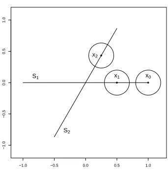
In our numerical experiments, we tried working both directly with covariance matrices as in (2) and with projections as in (3). Note that in our experiments we used spectral graph partitioning with soft versions of these affinities, as described in Section 2.2.4. We found working with projections to be more reliable. The problem comes, in part, from boundaries. When a surface has a boundary, local covariances over neighborhoods that overlap with the boundary are quite different from local covariances over nearby neighborhoods that do not touch the boundary. Consider the example of two segments, S1 and S2, intersecting at an angle ofθ∈(0, π/2) at their middle point, specifically
S1 = [−1,1]× {0}, S2 ={(x, xtanθ) :x∈[−cosθ,cosθ]}.
Assume there is no noise and that the sampling is uniform. Assume r ∈ (0,12sinθ) so that the disc centered at x1 := (1/2,0) does not intersect S2, and the disc centered at x2 := (12cosθ,12sinθ) does not intersect S1. Let x0 = (1,0). For x ∈ S1∪S2, let Cx denote the local covariance atxover a ball of radius r < 12sinθ, so that the neighborhoods of x0,x1,x2 are “pure”. The situation is described in Figure 2.
Simple calculations yield
Cx0 =
r2
12
1 0 0 0
, Cx1 =
r2
3
1 0 0 0
, Cx2 =
r2
3
cos2θ sin(θ) cos(θ) sin(θ) cos(θ) sin2θ
,
so that
kCx0−Cx1k=
r2
, kCx1−Cx2k=
r2
−1.0 −0.5 0.0 0.5 1.0
−1.0
−0.5
0.0
0.5
1.0
● ● ●
S1
S2
x0 x1 x2
Figure 2: Two segments intersecting. The local covariances (within the disc neighborhoods drawn) at x1 and x2 are closer than the local covariances at x1 and x0, even thoughx0 and x1 are on the same segment.
Therefore, when sinθ ≤ 34 (roughly, θ ≤ 48o), the local covariances at x0,x1 ∈ S1 are farther (in operator norm) than those atx1∈S1 andx2∈S2. As for projections, however,
Qx0 =Qx1 =
1 0 0 0
, Qx2 =
cos2θ sin(θ) cos(θ) sin(θ) cos(θ) sin2θ
,
so that
kQx0−Qx1k= 0, kQx1−Qx2k= √
2 sinθ.
While in theory points within distancer from the boundary account for a small portion of the sample, in practice this is not the case, at least not with the sample sizes that we are able to rapidly process. In fact, we find that spectral graph partitioning is challenged by having points near the boundary that are far (in affinity) from nearby points from the same cluster. This may explain why the (soft version of) affinity (3) yields better results than the (soft version of) affinity (2) in our experiments.
2.2.4 Spectral Clustering Based on Local PCA
The following variant is more robust in practice and is the algorithm we actually imple-mented. The method assumes that the surfaces are of same dimensiondand that there are
K of them, with both parametersK and dknown.
Spectral Clustering Based on Local PCA
Algorithm 4 Spectral Clustering Based on Local PCA Input:
Data pointsx1, . . . ,xn; neighborhood radiusr >0; spatial scale ε >0, projection scale
η >0; intrinsic dimensiond; number of clustersK.
Steps:
0: Pick one point y1 at random from the data. Pick another point y2 among the data points not included in Nr(y1), and repeat the process, selecting centersy1, . . . ,yn0.
1: For each i= 1, . . . , n0, compute the sample covariance matrix Ci of Nr(yi). Let Qi denote the orthogonal projection onto the space spanned by the topdeigenvectors ofCi.
2: Compute the following affinities between center pairs:
Wij = exp −
kyi−yjk2
ε2
!
·exp −kQi−Qjk 2
η2
!
. (4)
3: Apply spectral graph partitioning (Algorithm 1) toW.
4: The data points are clustered according to the closest center in Euclidean distance.
2.2.5 Comparison with Closely Related Methods
We highlight some differences with the other proposals in the literature. We first compare our approach to that of Goldberg et al. (2009), which was our main inspiration.
• Neighborhoods. Comparing with Goldberg et al. (2009), we define neighborhoods over
r-balls instead of `-nearest neighbors, and connect points over ε-balls instead of m -nearest neighbors. This choice is for convenience, as these ways are in fact essentially equivalent when the sampling density is fairly uniform. This is elaborated at length in (Maier et al., 2009; Brito et al., 1997; Arias-Castro, 2011).
• Mahalanobis distances. Goldberg et al. (2009) use Mahalanobis distances (1) between
centers. In our version, we could for example replace the Euclidean distancekxi−xjk in the affinity (2) with the average Mahalanobis distance
kC−1i /2(xi−xj)k+kC −1/2
j (xj−xi)k.
We actually tried this and found that the algorithm was less stable, particularly under low noise. Introducing a regularization in this distance—which requires the introduction of another parameter—solves this problem, at least partially.
That said, using Mahalanobis distances makes the procedure less sensitive to the choice of ε, in that neighborhoods may include points from different clusters. Think of two parallel line segments separated by a distance of δ, and assume there is no noise, so the points are sampled exactly from these segments. Assuming an infinite sample size, the local covariance is the same everywhere so that points within distance
version based on these distances would work with any ε > 0. In the case of curved surfaces and/or noise, the situation is similar, though not as evident. Even then, the gain in performance is not obvious since we only require that ε be slightly larger in order of magnitude thanr.
• Hellinger distances. As we mentioned earlier, Goldberg et al. (2009) use Hellinger dis-tances of the probability distributionsN(0,Ci) andN(0,Cj) to compare covariance matrices, specifically
1−2D/2 det(CiCj) 1/4 det(Ci+Cj)1/2
!1/2
, (5)
if Ci and Cj are full-rank. While using these distances or the Frobenius distances makes little difference in practice, we find it easier to work with the latter when it comes to proving theoretical guarantees. Moreover, it seems more natural to assume a uniform sampling distribution in each neighborhood rather than a normal distribution, so that using the more sophisticated similarity (5) does not seem justified.
• K-means. We use K-means++ for a good initialization. We found that the more
sophisticated size-constrained K-means (Bradley et al., 2000) used in (Goldberg et al., 2009) did not improve the clustering results.
As we mentioned above, our work was developed in parallel to that of Wang et al. (2011) and Gong et al. (2012). We highlight some differences. First, there is no subsampling, but rather, the local tangent space is estimated at each data point xi. Wang et al. (2011) fit a mixture of d-dimensional affine subspaces to the data using MPPCA (Tipping and Bishop, 1999), which is then used to estimate the tangent subspaces at each data point. Gong et al. (2012) develop some sort of robust local PCA. While Wang et al. (2011) assume all surfaces are of same dimension known to the user, Gong et al. (2012) estimate that locally by looking at the largest gap in the spectrum of estimated local covariance matrix. This is similar in spirit to what is done in Step 2 of Algorithm 3, but we did not include this step in Algorithm 4 because we did not find it reliable in practice. We also tried estimating the local dimensionality using the method of Little et al. (2009), but this failed in the most complex cases.
Wang et al. (2011) use a nearest-neighbor graph and their affinity is defined as
Wij = ∆ij· d
Y
s=1
cosθs(i, j)
!α
,
where ∆ij = 1 if xi is among the `-nearest neighbors of xj, or vice versa, while ∆ij = 0 otherwise; θ1(i, j)≥ · · · ≥ θd(i, j) are the principal (a.k.a., canonical) angles (Stewart and Sun, 1990) between the estimated tangent subspaces atxi andxj. `and α are parameters of the method. Gong et al. (2012) define an affinity that incorporates the self-tuning method of Zelnik-Manor and Perona (2005); in our notation, their affinity is
exp
−kxi−xjk 2
εiεj
·exp −(sin −1(kQ
i−Qjk))2
η2kx
i−xjk2/(εiεj)
!
Spectral Clustering Based on Local PCA
whereεi is the distance from xi to its `-nearest neighbor. `is a parameter.
Although we do not analyze their respective ways of estimating the tangent subspaces, our analysis provides essential insights into their methods, and for that matter, any other method built on spectral clustering based on tangent subspace comparisons.
3. Mathematical Analysis
While the analysis of Algorithm 4 seems within reach, there are some complications due to the fact that points near the intersection may form a cluster of their own—we were not able to discard this possibility. Instead, we study the simpler variants described in Algorithm 2 and Algorithm 3. Even then, the arguments are rather complex and interestingly involved. The theoretical guarantees that we obtain for these variants are stated in Theorem 1 and proved in Section 6. We comment on the analysis of Algorithm 4 right after that. We note that there are very few theoretical results on resolving intersecting manifolds—in fact, we are only aware of (Arias-Castro et al., 2011) (under severe restrictions on the dimension of the intersection). Some such results have been established for a number of methods for subspace clustering (affine surfaces), for example, in (Chen and Lerman, 2009b; Soltanolkotabi and Cand`es, 2012; Soltanolkotabi et al., 2014; Wang and Xu, 2013; Heckel and B¨olcskei, 2013; Tsakiris and Vidal, 2015; Ma et al., 2008).
The generative model we assume is a natural mathematical framework for multi-manifold learning where points are sampled in the vicinity of smooth surfaces embedded in Euclidean space. For concreteness and ease of exposition, we focus on the situation where two surfaces (i.e., K = 2) of same dimension 1 ≤ d ≤ D intersect. This special situation already contains all the geometric intricacies of separating intersecting clusters. On the one hand, clusters of different intrinsic dimension may be separated with an accurate estimation of the local intrinsic dimension without further geometry involved (Haro et al., 2007). On the other hand, more complex intersections (3-way and higher) complicate the situation without offering truly new challenges. For simplicity of exposition, we assume that the surfaces are submanifolds without boundary, though it will be clear from the analysis (and the experiments) that the method can handle surfaces with (smooth) boundaries that may self-intersect. We discuss other possible extensions in Section 5.
Within that framework, we show that Algorithm 2 and Algorithm 3 are able to identify the clusters accurately except for points near the intersection. Specifically, with high prob-ability with respect to the sampling distribution, Algorithm 2 divides the data points into two groups such that, except for points within distance Cε of the intersection, all points from the first cluster are in one group and all points from the second cluster are in the other group. The constant C depends on the surfaces, including their curvatures, separa-tion between them and intersecsepara-tion angle. The situasepara-tion for Algorithm 3 is more complex, as it may return more than two clusters, but most of the two clusters (again, away from the intersection) are in separate connected components.
3.1 Generative Model
Each surface we consider is a connected, C2 and compact submanifold without boundary and of dimensiondembedded inRD. Any such surface has a positive reach, which is what
Intuitively, a surface has reach exceeding r if and only if one can roll a ball of radiusr on the surface without obstruction (Walther, 1997; Cuevas et al., 2012). Formally, forx∈RD
and S⊂RD, let
dist(x, S) = inf
s∈Skx−sk, and
B(S, r) ={x: dist(x, S)< r},
which is often called the r-tubular neighborhood (or r-neighborhood) of S. The reach of
S is the supremum over r > 0 such that, for each x∈ B(S, r), there is a unique point in
S nearest x. It is well-known that, for C2 submanifolds, the reach bounds the radius of curvature from below (Federer, 1959, Lem. 4.17). For submanifolds without boundaries, the reach coincides with the condition number introduced in (Niyogi et al., 2008).
When two surfaces S1 and S2 intersect, meaningS1∩S26=∅, we define their incidence angle as
θ(S1, S2) := inf
θmin(TS1(s), TS2(s)) :s∈S1∩S2 , (6)
whereTS(s) denote the tangent subspace of submanifoldSat points∈S, andθmin(T1, T2) is the smallestnonzeroprincipal (a.k.a., canonical) angle between subspacesT1 andT2 (Stew-art and Sun, 1990).
The clusters are generated as follows. Each data point xi is drawn according to
xi =si+zi, (7)
where si is drawn from the uniform distribution over S1∪S2 and zi is an additive noise term satisfyingkzik ≤τ—thusτ represents the noise or jitter level. Whenτ = 0 the points are sampled exactly on the surfaces. We assume the points are sampled independently of each other. We let
Ik={i:si∈Sk},
and the goal is to recover the groupsI1 and I2, up to some errors. 3.2 Performance Guarantees
We state some performance guarantees for Algorithm 2 and Algorithm 3.
Theorem 1. Consider two connected, compact, twice continuously differentiable submani-folds without boundary, of same dimension d, intersecting at a strictly positive angle, with the intersection set having strictly positive reach. Assume the parameters are set so that
τ ≤rη/C, r ≤ε/C, ε≤η/C, η≤1/C, (8)
for a large-enough constant C≥1that depends on the configuration. Then with probability
at least 1−Cnexp
−nrdη2/C :
• Algorithm 2 returns exactly two groups such that two points from different clusters are
not grouped together unless one of them is within distance Cr from the intersection.
Spectral Clustering Based on Local PCA
Thus, as long as, (8) is satisfied, the algorithms have the above properties with high probability when rdη2 ≥ C0logn/n, where C0 > C is fixed. In particular, we may choose
η1 andεr τ ∨(log(n)/n)1/d, which lightens the computational burden.
We note that, while the constantC >0 does not depend on the sample sizen, it depends in somewhat complicated ways on characteristics of the surfaces and their position relative to each other, such as their reach and intersection angle, but also aspects that are harder to quantify, like their separation away from their intersection. We note, however, that it behaves as expected: C is indeed decreasing in the reach and the intersection angle, and increasing in the intrinsic dimensions of the surfaces, for example.
The algorithms may make clustering mistakes within distance Cr of the intersection, whereCrτ∨(log(n)/n)1/dwith the choice of parameters just described. Whether this is optimal in the nonparametric setting that we consider—for example, in a minimax sense— we do not know.
We now comment on the challenge of proving a similar result for Algorithm 4. This algorithm relies on knowledge of the intrinsic dimension of the surfacesdand the number of clusters (hereK= 2), but these may be estimated as in (Arias-Castro et al., 2011), at least in theory, so we assume these parameters are known. The subsampling done in Step 0 does not pose any problem whatsoever, since the centers are well-spread when the points themselves are. The difficulty resides in the application of the spectral graph partitioning, Algorithm 1. If we were to include the intersection-removal step (Step 2 of Algorithm 2) before applying spectral graph partitioning, then a simple adaptation of arguments in (Arias-Castro, 2011) would suffice. The real difficulty, and potential pitfall of the method in this framework (without the intersection-removal step), is that the points near the intersection may form their own cluster. For example, in the simplest case of two affine surfaces intersecting at a positive angle and no sampling noise, the projection matrix at a point near the intersection— meaning a point whose r-ball contains a substantial piece of both surfaces—would be the projection matrix onto S1 +S2 seen as a linear subspace. We were not able to discard this possibility, although we do not observe this happening in practice. A possible remedy is to constrain the K-means part to only return large-enough clusters. However, a proper analysis of this would require a substantial amount of additional work and we did not engage seriously in this pursuit.
4. Numerical Experiments
4.1 Some Illustrative Examples
We started by applying our method2 on a few artificial examples to illustrate the theory. As we argued earlier, the methods of Wang et al. (2011) and Gong et al. (2012) are quite similar to ours, and we encourage the reader to also look at the numerical experiments they performed. Our numerical experiments should be regarded as a proof of concept, only here to show that our method can be implemented and works on some stylized examples.
In all experiments, the number of clusters K and the dimension of the manifolds dare assumed known. We choose the spatial scaleεand the projection scale η automatically as
follows: we let
ε= max 1≤i≤n0
min
j6=i kyi−yjk, (9)
and
η= median (i,j):kyi−yjk<ε
kQi−Qjk.
Here, we implicitly assume that the union of all the underlying surfaces forms a connected set. In that case, the idea behind choosing ε as in (9) is that we want theε-graph on the centersy1, . . . ,ynto be connected. Thenη is chosen so that a centeryi remains connected in the (ε, η)-graph to most of its neighbors in the ε-graph.
The neighborhood radius r is chosen by hand for each situation. Although we do not know how to choose r automatically, there are some general ad hoc guidelines. When r
is too large, the local linear approximation to the underlying surfaces may not hold in neighborhoods of radius r, resulting in local PCA becoming inappropriate. When r is too small, there might not be enough points in a neighborhood of radius r to accurately estimate the local tangent subspace to a given surface at that location, resulting in local PCA becoming inaccurate. From a computational point of view, the smaller r, the larger the number of neighborhoods and the heavier the computations, particularly at the level of spectral graph partitioning. In our numerical experiments, we find that our algorithm is more sensitive to the choice of r when the clustering problem is more difficult. We note that automatic choice of tuning parameters remains a challenge in clustering, and machine learning at large, especially when no labels are available whatsoever. See (Zelnik-Manor and Perona, 2005; Zhang et al., 2012; Little et al., 2009; Kaslovsky and Meyer, 2011).
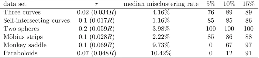
Since the algorithm is randomized (see Step 0 in Algorithm 4) we repeat each simula-tion 100 times and report the median misclustering rate and number of times where the misclustering rate is smaller than 5%, 10%, and 15%.
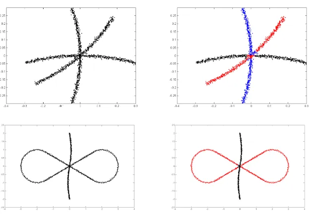
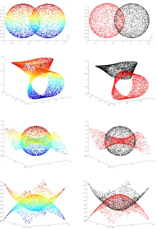
We first run Algorithm 4 on several artificial data sets, which are demonstrated in the LHS of Figures 3 and 4. Table 1 reports the local radiusr used for each data set (R is the global radius of each data set), and the statistics for misclustering rates. Typical clustering results are demonstrated in the RHS of Figures 3 and 4. It is evident that Algorithm 4 performs well in these simulations.
data set r median misclustering rate 5% 10% 15% Three curves 0.02 (0.034R) 4.16% 76 89 89 Self-intersecting curves 0.1 (0.017R) 1.16% 85 85 86 Two spheres 0.2 (0.059R) 3.98% 100 100 100 M¨obius strips 0.1 (0.028R) 2.22% 85 86 88 Monkey saddle 0.1 (0.069R) 9.73% 0 67 97 Paraboloids 0.07 (0.048R) 10.42% 0 12 91
Spectral Clustering Based on Local PCA
Figure 3: Performance of Algorithm 4 on data sets “Three curves” and “Self-intersecting curves”. Left column is the input data sets, and right column demonstrates the typical clustering.
In another simulation, we show the dependence of the success of our algorithm on the intersecting angle between curves in Table 2 and Figure 5. Here, we fix two curves intersecting at a point, and gradually decrease the intersection angle by rotating one of them while holding the other one fixed. The angles are π/2, π/4, π/6 and π/8. From the table we can see that our algorithm performs well when the angle is π/4, but the performance deteriorates as the angle becomes smaller, and the algorithm almost always fails when the angle isπ/8.
Intersecting angle r median misclustering rate 5% 10% 15%
π/2 0.02 (0.034R) 2.08% 98 98 98
π/4 0.02 (0.034R) 3.33% 92 94 94
π/6 0.02 (0.034R) 5.53% 32 59 59
π/8 0.02 (0.033R) 27.87% 0 2 2
Spectral Clustering Based on Local PCA
4.2 Comparison with Other Multi-manifold Clustering Algorithms
In this section, we compare our algorithm with several existing algorithms on multi-manifold clustering. While many algorithms have been proposed, we focus on the methods based on spectral clustering, including Sparse Manifold Clustering and Embedding (SMCE) (Elham-ifar and Vidal, 2011) and Local Linear Embedding of (Polito and Perona, 2001; Goh and Vidal, 2007). Compared to these methods, a major difference of Algorithm 4 is the size of the affinity matrix W: SMCE and LLE each creates ann×naffinity matrix while our method creates a smaller affinity matrix of sizen0×n0, based on the centers chosen in step 0 of Algorithm 4. This difference enables our algorithm to handle large data sets such as
n > 104, while these other two methods are computationally expensive due to eigenvalue decomposition of the n×n affinity matrix. In order to make a fair comparison, we will run simulations and experiments on small data sets. We modified our algorithm to make it more competitive in such a setting: we modify Steps 0 and 1 in Algorithm 4 slightly and use all data points {xi}ni=1 as centers, that is, yi =xi for all 1≤i≤n. The motivation is that, when there is no computational constraint on the eigenvalue decomposition (due to smalln), we may improve Algorithm 4 by constructing a larger affinity matrix by including all points as centers. The resulting algorithm is summarized in Algorithm 5.
Algorithm 5 Spectral Clustering Based on Local PCA (for small data sets) Input:
Data points x1, . . . ,xn; neighborhood size N > 0; spatial scale ε > 0, projection scale
η >0; intrinsic dimensiond; number of clustersK.
Steps:
1: For eachi= 1, . . . , n, compute the sample covariance matrixCiof from theN nearest neighbors of xi. Let Qi denote the orthogonal projection onto the space spanned by the topdeigenvectors ofCi.
2: Compute the following affinities between ndata points:
Wij = exp
−kxi−xjk 2
ε2
·exp −kQi−Qjk 2
η2
!
.
3: Apply spectral graph partitioning (Algorithm 1) toW.
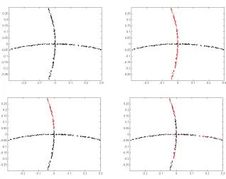
First we test the algorithms on a simulated data set of two curves, which is subsampled from the first data set in Figure 5 with 300 data points. We plot the clustering result from Algorithm 5, SMCE, LLE in Figure 6. For Algorithm 5, K is set to be 10. For SMCE3,
λ = 10 and L = 60, and we remark that similar results are obtained for a wide range of parameters. For LLE, we follow the implementation in (Polito and Perona, 2001), use 10-nearest neighbors to embed the data set into R2 and runK-means on the embedded data
set. It is clear from the figure that Algorithm 5 resolves the problem of intersection well
3. In (Elhamifar and Vidal, 2011), λ is the `1-penalty parameter and at each point the optimization is
Spectral Clustering Based on Local PCA
Figure 6: Performance of Algorithm 5 on two intersecting curves. Left top: the input data set. Right top: the clustering result by Algorithm 5. Left bottom: the clustering result by SMCE. Right bottom: the clustering result by LLE.
by using the affinity from estimated local subspaces, while SMCE and LLE tend to give a larger affinity between nearby data points and have difficulties in handling intersection.
Next, we run experiments on the Extended Yale Face Database B (Lee et al., 2005), with the goal of clustering face images of two different subjects. This data set contains face images from 39 subjects, and each subject has 64 images of 192 pixels under varying lightening conditions. In our experiments, we found that the images of a person in this database lie roughly in a 4-dimensional subspace. We preprocess the data set by applying PCA and reducing the dimension to 8. We also “normalize” the covariance of the data set when performing dimension reduction, such that the projected data set has a unit covariance. We record the misclustering rates of Algorithm 5, SMCE and LLE in Table 3. For SMCE, we follow (Elhamifar and Vidal, 2011) by setting λ = 10 and we let L = 30. For Algorithm 5, we let the neighborhood size be 40. From the table, we can see that the two methods perform similarly.
subjects [1,2] [1,3] [1,4] [1,5] [1,6] [1,7] [1,8] [1,9] Local PCA 8.59% 11.72% 10.94% 4.69% 8.59% 7.81% 5.47% 7.03% SMCE 8.59% 11.72% 8.59% 0.00% 4.69% 8.59% 9.38% 4.69%
5. Discussion
We distilled the ideas of Goldberg et al. (2009) and of Kushnir et al. (2006) to cluster points sampled near smooth surfaces. The key ingredient is the use of local PCA to learn about the local spread and orientation of the data, so as to use that information in an affinity when building a neighborhood graph.
In a typical stylized setting for multi-manifold clustering, we established performance bounds for the simple variants described in Algorithm 2 and Algorithm 3, which essentially consist of connecting points that are close in space and orientation, and then extracting the connected components of the resulting graph. Both are shown to resolve general inter-sections as long as the incidence angle is strictly positive and the parameters are carefully chosen. As is commonly the case in such analyses, our setting can be generalized to other sampling schemes, to multiple intersections, to some features of the surfaces changing with the sample size, and so on, in the spirit of (Arias-Castro et al., 2011; Arias-Castro, 2011; Chen and Lerman, 2009b). We chose to simplify the setup as much as possible while taining the essential features that make resolving intersecting clusters challenging. The re-sulting arguments are nevertheless rich enough to satisfy the mathematically thirsty reader. Whether the conditions required in Theorem 1 are optimal in some sense is an interesting and challenging open question for future research. Note that very few optimality results exist for manifold clustering; see (Arias-Castro, 2011) for an example.
We implemented a spectral version of Algorithm 3, described in Algorithm 4, that assumes the intrinsic dimensionality and the number of clusters are known. The resulting approach is very similar to what is offered by Wang et al. (2011) and Gong et al. (2012), although it was developed independently of these works. Algorithm 4 is shown to perform well in some simulated experiments, although it is somewhat sensitive to the choice of parameters. This is the case of all other methods for multi-manifold clustering we know of and choosing the parameters automatically remains an open challenge in the field.
6. Proofs
We start with some additional notation. The ambient space is RD unless noted otherwise.
For a vector v ∈ RD, kvk denotes its Euclidean norm and for a real matrixM ∈
RD×D,
kMk denotes the corresponding operator norm. For a point x ∈ RD and r > 0, B(x, r)
denotes the open ball of centerxand radius r, i.e.,B(x, r) ={y∈RD :ky−xk< r}. For a setS and a pointx, define dist(x, S) = inf{kx−yk:y∈S}. For two points a,bin the same Euclidean space, b−a denotes the vector movinga tob. For a pointa and a vector v in the same Euclidean space,a+v denotes the translate ofa byv. We identify an affine subspaceT with its corresponding linear subspace, for example, when saying that a vector belongs to T.
For two subspaces T andT0, of possibly different dimensions, let 0≤θmax(T, T0)≤π/2 denote the largest and byθmin(T, T0) the smallest nonzero principal angle betweenT andT0 (Stewart and Sun, 1990). Whenv is a vector and T is a subspace,∠(v, T) :=θmax(Rv, T)
Spectral Clustering Based on Local PCA
For a subset A⊂ RD and positive integer d, vol
d(A) denotes the d-dimensional Haus-dorff measure of A, and vol(A) is defined as voldim(A)(A), where dim(A) is the Hausdorff dimension ofA. For a Borel set A, let λAdenote the uniform distribution on A.
For a setS ⊂RD with reach at least 1/κ, andxwith dist(x, S)<1/κ, letPS(x) denote the metric projection ofxontoS, that is, the point onS closest tox. Note that, ifT is an affine subspace, then PT is the usual orthogonal projection onto T, and we let PT denote the orthogonal projection onto the linear subspace of same dimension and parallel toT. Let Sd(κ) denote the class of connected,C2 and compact d-dimensional submanifolds without boundary embedded inRD, with reach at least 1/κ. For a submanifold S ∈RD, let TS(x) denote the tangent space of S atx∈S.
We will often identify a linear map with its matrix in the canonical basis. For a sym-metric (real) matrix M, let β1(M) ≥ β2(M) ≥ · · · denote its eigenvalues in decreasing order.
We say that f : Ω⊂RD →
RD isC-Lipschitz if kf(x)−f(y)k ≤Ckx−yk,∀x,y∈Ω.
For two reals aand b,a∨b= max(a, b) and a∧b= min(a, b). Additional notation will be introduced as needed.
6.1 Preliminaries
This section gathers a number of general results from geometry and probability. We took time to package them into standalone lemmas that could be of potential independent inter-est, particularly to researchers working in machine learning and computational geometry. When needed, we useC to denote a constant that may change with each appearance.
6.1.1 Smooth Surfaces and Their Tangent Subspaces
The following comes directly from (Federer, 1959, Th. 4.18(12)). It gives us a simple criterion for identifying the metric projection of a point on a surface with given reach.
Lemma 1. Consider S ∈ Sd(κ) and x∈RD such that dist(x, S) <1/κ. Then s=PS(x)
if and only if kx−sk<1/κand x−s⊥TS(s).
The following result is on approximating a smooth surface near a point by the tangent subspace at that point. It is based on (Federer, 1959, Th. 4.18(2)).
Lemma 2. ForS ∈ Sd(κ), and any two pointss,s0 ∈S,
dist(s0, TS(s))≤
κ
2ks 0−
sk2, (10)
and when dist(s0, TS(s))≤1/κ,
dist(s0, TS(s))≤κkPTS(s)(s
0)−sk2. (11)
Moreover, for t∈TS(s) such that ks−tk ≤ 31κ,
Proof. Let T be short forTS(s). (Federer, 1959, Th. 4.18(2)) says that
dist(s0−s, T)≤ κ 2ks
0−sk2. (13)
Immediately, we have
dist(s0−s, T) =ks0−PT(s0)k= dist(s0, T),
and (10) comes from that. Based on that and Pythagoras theorem, we have
dist(s0, T) =kPT(s0)−s0k ≤
κ
2ks
0−sk2= κ
2 kPT(s
0)−s0k2+kP
T(s0)−sk2
,
so that
dist(s0, T) 1−κ 2dist(s
0
, T)≤ κ 2kPT(s
0
)−sk2,
and (11) follows easily from that. For (12), letr = 1/(3κ) ands0 =PT−1(t), the latter being well-defined by Lemma 5 below and belongs to B(s, r(1 +κr)) ⊂ B(s,4/(9κ)). By (10), ks0−sk ≤8/(81κ)<1/κ, and by (11),
dist(t, S)≤ kt−s0k= dist(s0, T)≤κkt−sk2.
This concludes the proof of (12).
We will need a bound on the angle between tangent subspaces on a smooth surface as a function of the distance between the corresponding points of contact.
Lemma 3 (Boissonnat et al. (2013)). ForS ∈ Sd(κ), and any s,s0 ∈S,
sinθmax(TS(s), TS(s0))≤6κks0−sk. (14) The following bounds the difference between the metric projection onto a surface and the orthogonal projection onto one of its tangents.
Lemma 4. ConsiderS ∈ Sd(κ) ands∈S. Then for any x∈B(S, r), we have
kPS(x)−PTS(s)(x)k ≤C4κkx−sk
2,
for a numeric constant C4 >0.
Proof. Let T = TS(s) and define t = PT(x), s0 = PS(x) and ˜t = PT(s0), and also T0 =
TS(s0) and θ=θmax(T, T0). We have
PS(x) =PT0(x) =PT0(x−s0) +s0
PT(x) =PT(x−˜t) + ˜t=PT(x−s0) +PT(s0−˜t) + ˜t.
Hence,
Spectral Clustering Based on Local PCA
On the one hand,
kPT(s0−˜t)k ≤ ks0−˜tk= dist(s0, T)≤
κ
2ks 0−
sk2 ≤2κkx−sk2,
by (10) and the fact that
ks0−sk ≤ ks0−xk+kx−sk= dist(x, S) +kx−sk ≤2kx−sk.
On the other hand, applying Lemma 18 (see further down)
kPT0(x−s0)−PT(x−s0)k ≤ kPT0−PTkkx−s0k= (sinθ)kx−s0k,
withkx−s0k ≤ kx−skand, applying Lemma 3,
sinθ≤6κks0−sk ≤12κkx−sk.
All together, we conclude.
Below we state some properties of a projection onto a tangent subspace. A result similar to the first part was proved in (Arias-Castro et al., 2011, Lem. 2) based on results in (Niyogi et al., 2008), but the arguments are simpler here and the constants are sharper.
Lemma 5. There is a numeric constant C5 ≥ 1 such that the following holds. Take S ∈ Sd(κ),s∈S andr≤1/C5κ, and letT be short forTS(s). PT is injective onB(s, r)∩S and
its image contains B(s, r0)∩T, where r0 := (1−C5(κr)2)r. Moreover, PT−1 has Lipschitz constant bounded by 1 +C5(κr)2≤1 +κr over B(s, r)∩T.
Proof. Takes0,s00∈Sdistinct such thatPT(s0) =PT(s00). Equivalently,s00−s0is perpendic-ular toT. Let T0 be short forTS(s0). By (13) and the fact that dist(v, T) =kvksin∠(v, T) for any vectorv and any linear subspace T, we have
sin∠(s00−s0, T0)≤ κ 2ks
00−s0k,
and by (14),
sinθmax(T, T0)≤6κks−s0k. Now, by the triangle inequality,
π
2 =∠(s
00−s0, T)≤
∠(s00−s0, T0) +θmax(T, T0), so that
κ
2ks
00−s0k ∧1≥ π 2 −sin
−1 6κks0−sk ∧1
.
When ks0−sk ≤1/12κ, the RHS is bounded from below by π/2−sin−1(1/2), which then implies that κ2ks00−s0k ≥sin(π/2−sin−1(1/2)) =√3/2, that is, ks00−s0k ≥√3/κ. This precludes the situation where s0,s00∈B(s,1/12κ), so thatPT is injective on B(s, r) when
r≤1/12κ.
The same arguments imply that PT is an open map on R:=B(s, r)∩S. In particular,
∂B(s, r) since ∂S = ∅. Now take any ray out of s within T, which is necessarily of the form s+R+v, where v is a unit vector in T. Let ta =s+av ∈ T fora∈[0,∞). Leta∗ be the infimum over all a >0 such that ta ∈PT(R). Note that a∗ >0 and ta∗ ∈PT(∂R),
so that there is s∗ ∈ ∂R such that PT(s∗) =ta∗. Let sa =P
−1
T (ta), which is well-defined on [0, a∗] by definition of a∗ and the fact that PT is injective on R. Let Jt denote the differential of PT−1 att. We have that ˙sa=Jtav is the unique vector in Ta:=TS(sa) such
thatPT( ˙sa) =v. Elementary geometry shows that
kPT( ˙sa)k=ks˙akcos∠( ˙sa, T)≥ ks˙akcosθmax(Ta, T), with
cosθmax(Ta, T)≥cos
sin−1(6κksa−sk ∧1)
≥ζ := 1−(6κr)2,
by (14) and fact that ksa−sk ≤r (and assuming 6κr≤1). SincekPT( ˙sa)k=kvk= 1, we haveks˙ak ≤1/ζ,and this holds for alla < a∗. So we can extendsato [0, a∗] into a Lipschitz function with constant 1/ζ. Together with the fact that s∗ ∈∂B(s, r), this implies that
r=ks∗−sk=ksa∗−s0k ≤a∗/ζ.
Hence,a∗≥ζrand therefore PT(R) containsB(s, ζr)∩T as stated.
For the last part, assume r ≤ 1/Cκ, with C large enough that there is a unique h ≤ 1/12κ such thatζh=r, where ζ is redefined as ζ := 1−(6κh)2. Take t0 ∈B(s, r)∩T and let s0 =PT−1(t0) and T0 =TS(s0). We saw that PT−1 is Lipschitz with constant 1/ζ on any ray emanating from s of length ζh=r, so that ks0−sk ≤(1/ζ)kt0−sk ≤ r/ζ =h. The differential of PT at s0 is PT itself, seen as a linear map between T0 and T. Then for any vectoru∈T0, we have
kPT(u)k=kukcos∠(u, T)≥ kukcosθmax(T0, T), with
cosθmax(T0, T)≥cossin−1 6κks0−sk
≥1−(6κh)2 =ζ,
as before. Hence, kJt0k ≤ 1/ζ, and we proved this for all t0 ∈ B(s, r)∩T. This last set
being convex, we can apply Taylor’s theorem and get thatPT−1 is Lipschitz on that set with constant 1/ζ. We then note thatζ = 1 +O(κr)2.
6.1.2 Volumes and Uniform Distributions
Below is a result that quantifies how much the volume of a set changes when applying a Lipschitz map. This is well-known in measure theory and we only provide a proof for completeness.
Lemma 6. Suppose Ωis a measurable subset of RD andf : Ω⊂RD →RD isC-Lipschitz.
Then for any measurable set A⊂Ω and real d >0, vold(f(A))≤Cdvold(A).
Proof. By definition,
vold(A) = lim t→0 V
t
d(A), Vdt(A) := inf (Ri)∈Rt(A)
X
i∈N
Spectral Clustering Based on Local PCA
where Rt(A) is the class of countable sequences (R
i : i ∈ N) of subsets of RD such that
A⊂S
iRi and diam(Ri)< tfor all i. Sincef is C-Lipschitz, diam(f(R))≤Cdiam(R) for any R⊂Ω. Hence, for any (Ri)∈ Rt(A), (f(Ri))∈ RCt(f(A)). This implies that
VdCt(f(A))≤X i∈N
diam(f(Ri))d≤Cd
X
i∈N
diam(Ri)d.
Taking the infimum over (Ri) ∈ Rt(A), we get VdCt(f(A)) ≤ CdVdt(A), and we conclude by taking the limit as t → 0, noticing that VdCt(f(A)) → vold(f(A)) while Vdt(A) → vold(A).
We compare below two uniform distributions. For two Borel probability measures P
and Qon RD, TV(P, Q) denotes their total variation distance, meaning,
TV(P, Q) = sup{|P(A)−Q(A)|:A Borel}.
Remember that for a Borel setA, λA denotes the uniform distribution onA.
Lemma 7. Suppose A and B are two Borel subsets of RD. Then
TV(λA, λB)≤4
vol(A4B) vol(A∪B).
Proof. IfA andB are not of same dimension, say dim(A)>dim(B), then TV(λA, λB) = 1 sinceλA(B) = 0 while λB(B) = 1. And we also have
vol(A4B) = voldim(A)(A4B) = voldim(A)(A) = vol(A), and
vol(A∪B) = voldim(A)(A∪B) = voldim(A)(A) = vol(A), in both cases because voldim(A)(B) = 0. So the result works in that case.
Therefore assume that Aand B are of same dimension. Assume WLOG that vol(A)≥ vol(B). For any Borel setU,
λA(U)−λB(U) =
vol(A∩U) vol(A) −
vol(B∩U) vol(B) ,
so that
|λA(U)−λB(U)| =
vol(A∩U) vol(A) −
vol(B∩U) vol(A) +
vol(B∩U) vol(A) −
vol(B∩U) vol(B)
≤ |vol(A∩U)−vol(B∩U)| vol(A) +
vol(B∩U) vol(B)
|vol(A)−vol(B)| vol(A)
≤ 2 vol(A4B) vol(A) ,
We now look at the projection of the uniform distribution on a neighborhood of a surface onto a tangent subspace. For a Borel probability measure P and measurable function f :
RD →RD,Pf denotes the push-forward (Borel) measure defined byPf(A) =P(f−1(A)).
Lemma 8. Suppose A⊂RD is Borel andf :A→
RD is invertible on f(A), and that both
f andf−1 are C-Lipschitz. Then
TV(λfA, λf(A))≤2(Cdim(A)−1).
Proof. First, note thatAandf(A) are both of same dimension, and thatC ≥1 necessarily. Letdbe short for dim(A). Take U ⊂f(A) Borel and let V =f−1(U). Then
λfA(U) = vol(A∩V)
vol(A) , λf(A)(U) =
vol(f(A)∩U) vol(f(A)) ,
and as in (16),
|λfA(U)−λf(A)(U)| ≤ |vol(A∩V)−vol(f(A)∩U)| vol(A) +
|vol(A)−vol(f(A))| vol(A) .
f being invertible, we have f(A∩V) =f(A)∩U and f−1(f(A)∩U) =A∩V. Therefore, applying Lemma 6, we get
C−d≤ vol(f(A)∩U) vol(A∩V) ≤C
d,
so that
|vol(A∩V)−vol(f(A)∩U)| ≤(Cd−1) vol(A∩V)≤(Cd−1) vol(A).
And takingV =A, we also get
|vol(A)−vol(f(A))| ≤(Cd−1) vol(A).
From this we conclude.
Now comes a technical result on the intersection of a smooth surface and a ball.
Lemma 9. There is a constant C9 ≥ 3 depending only on d such that the following is
true. Take S ∈ Sd(κ), r < C1
9κ and x∈R
D such that dist(x, S) < κ. Let s= P
S(x) and
T =TS(s). Then
vol PT(S∩B(x, r))4(T∩B(x, r))
≤C9κ(kx−sk+κr2) vol(T ∩B(x, r)).
Proof. If dist(x, S) > r, then S ∩B(x, r) = T ∩B(x, r) = ∅, and if dist(x, S) = r, then
S∩B(x, r) = T ∩B(x, r) = {s}, and in both cases the inequality holds trivially. So it suffices to consider the case where dist(x, S)< r.
LetAr=B(s, r),Br =B(x, r) andg=PT for short. Note thatT∩Br=T∩Ar0 where
r0 := (r2−δ2)1/2 and δ := kx−sk. Take s1 ∈ S∩Br such that g(s1) is farthest from s, so that g(S∩Br)⊂Ar1 wherer1 :=ks−g(s1)k—note thatr1 ≤r. Let `1=ks1−g(s1)k
Spectral Clustering Based on Local PCA
we have kx−s1k2 = kx−y1k2 +ky1 −s1k2. We have kx−s1k ≤ r and ky1−s1k = ks−g(s1)k=r1. And because`1 ≤κr21 < rby (11), eithery1 is betweenxands, in which casekx−y1k=δ−`1, orsis betweenxandy1, in which casekx−y1k=δ+`1. In any case,
r2≥r12+ (δ−`1)2, which together with`1 ≤κr21 impliesr21 ≤r2−δ2+ 2δ`1≤r20+ 2κr21δ, leading to r1 ≤ (1−2κδ)−1/2r0 ≤ (1 + 4κδ)r0 after noticing that δ ≤ r < 1/(3κ). From
g(S∩Br)⊂T ∩Ar1, we get
vol g(S∩Br)\(T∩Br)
≤ vol(T∩Ar1)−vol(T ∩Ar0)
= ((r1/r0)d−1) vol(T∩Ar0).
We follow similar arguments to get a sort of reverse relationship. Takes2∈S∩Br such thatg(S∩Br)⊃T∩Ar2, wherer2 :=ks−g(s2)kis largest. Assumingris small enough, by
Lemma 5,g−1 is well-defined onT∩Ar, so that necessarilys2 ∈∂Br. Let`2 =ks2−g(s2)k and y2 be the orthogonal projection ofs2 onto the line (x,s). By Pythagoras theorem, we havekx−s2k2 =kx−y2k2+ky2−s2k2. We havekx−s2k=randky2−s2k=ks−g(s2)k=
r2. And by the triangle inequality, kx−y2k ≤ kx−sk+ky2 −sk = δ +`2. Hence,
r2≤r22+ (δ+`2)2, which together with`2≤κr22 by (11), impliesr22 ≥r2−δ2−2δ`2−`22≥
r02−(2δ +κr2)κr22, leading to r2 ≥ (1 + 2κδ+κ2r2)−1/2r0 ≥ (1−2κδ−κ2r2)r0. From
g(S∩Br)⊃T ∩Ar2, we get
vol (T∩Br)\g(S∩Br)
≤ vol(T∩Ar0)−vol(T ∩Ar2)
= (1−(r2/r0)d) vol(T∩Ar0).
All together, we have
vol g(S∩Br)4(T∩Br)
≤ (r1/r0)d−(r2/r0)d
vol(T ∩Ar0)
≤ (1 + 4κδ)d−(1−2κδ−κ2r2)dvol((T ∩Br)) ≤ Cdκ(δ+κr2) vol((T ∩Br)),
when δ≤r ≤1/(Cκ) and C is a large-enough numerical constant.
We bound below the d-volume of a the intersection of a ball with a smooth surface. Although it could be obtained as a special case of Lemma 9, we provide a direct proof because this result is at the cornerstone of many results in the literature on sampling points uniformly on a smooth surface.
Lemma 10. Suppose S∈ Sd(κ). Then for any s∈S and r < (d∨C15)κ, we have
1−2dκr≤ vol(S∩B(s, r))
vol(T∩B(s, r)) ≤1 + 2dκr,
where T :=TS(s) is the tangent subspace of S at s.
Proof. Let T =TS(s), Br =B(s, r) and g = PT for short. By Lemma 5, g is 1-Lipschitz and g−1 is (1 +κr)-Lipschitz onT ∩Br, so by Lemma 6 we have
Thatg−1 is Lipschitz with constant 1 +κrong(S∩Br) also implies thatg(S∩Br) contains
T∩Br0 wherer0 :=r/(1 +κr). From this, and the fact that g(S∩Br)⊂T∩Br, we get
1≤ vol(T ∩Br) vol(g(S∩Br))
≤ vol(T∩Br) vol(T∩Br0)
= r d
r0d = (1 +κr)
d.
We therefore have
vol(S∩Br)≥vol(g(S∩Br))≥(1 +κr)−dvol(T∩Br),
and
vol(S∩Br)≤(1 +κr)dvol(g(S∩Br))≤(1 +κr)dvol(T ∩Br).
And we conclude with the inequality (1 +x)d≤1 + 2dx valid for any x∈[0,1/d] and any
d≥1.
We now look at the density of a sample from the uniform on a smooth, compact surface.
Lemma 11. Consider S ∈ Sd(κ). There is a constant C11 >0 depending on S such that
the following is true. Sample n points s1, . . . ,sn independently and uniformly at random
from S. Take0< r <1/(C11κ). Then with probability at least 1−C11r−dexp(−nrd/C11),
any ball of radius r with center on S has between nrd/C11 andC11nrd sample points.
Proof. For a set R, let N(R) denote the number of sample points in R. For any R
measurable, N(R) ∼ Bin(n, pR), where pR := vol(R ∩S)/vol(S). Let x1, . . . ,xm be a maximal (r/2)-packing of S, and let Bi = B(xi, r/4)∩S. For any s ∈ S, there is i such that ks−xik ≤ r/2, which implies Bi ⊂ B(s, r) by the triangle inequality. Hence, mins∈SN(B(s, r))≥miniN(Bi).
By the fact that Bi∩Bj =∅ fori6=j,
vol(S)≥ m
X
i=1
vol(Bi)≥mmin
i vol(Bi),
and assuming thatκr is small enough, we have
min
i vol(Bi)≥
ωd 2 (r/4)
d,
by Lemma 10, whereωdis the volume of thed-dimensional unit ball. This leads tom≤Cr−d and p:= mini pBi ≥r
d/C, whenκr≤1/C, whereC >0 depends only onS.
Now, applying Bernstein’s inequality to the binomial distribution, we get
P(N(Bi)≤np/2)≤P(N(Bi)≤npBi/2)≤e
−(3/32)npBi ≤e−(3/32)np. We follow this with the union bound, to get
P
min
s∈SN(B(s, r))≤nr d/(2C)
≤me−(3/32)np≤ Cr−de−323Cnr d
.
Spectral Clustering Based on Local PCA
Next, we bound the volume of the symmetric difference between two balls.
Lemma 12. Take x,y∈Rd and 0< δ≤1. Then vol(B(x, δ)4B(y,1))
2 vol(B(0,1)) ≤1−(1− kx−yk) d +∧δd.
Proof. It suffices to prove the result when kx−yk <1. In that case, with γ := (1− kx− yk)∧δ, we have B(x, γ)⊂B(x, δ)∩B(y,1), so that
vol(B(x, δ)4B(y,1)) = vol(B(x, δ)) + vol(B(y,1))−2 vol(B(x, δ)∩B(y,1)) ≤ 2 vol(B(y,1))−2 vol(B(x, γ))
= 2 vol(B(0,1))(1−γd).
This concludes the proof.
6.1.3 Covariances
The result below describes explicitly the covariance matrix of the uniform distribution over the unit ball of a subspace.
Lemma 13. LetT be a subspace of dimensiond. Then the covariance matrix of the uniform distribution on T∩B(0, a) (seen as a linear map) is equal to a2cPT, where c:= d+21 .
Proof. Assume WLOG thatT =Rd× {0}. LetX be distributed according to the uniform
distribution on T∩B(0,1) and letR =kXk. Note that
P(R≤r) = vol(T ∩B(0, r))
vol(T∩B(0,1)) =r
d, ∀r ∈[0,1].
By symmetry,E(XiXj) = 0 if i6=j, while
E(X12) = 1
dE(X
2
1 +· · ·+Xd2) = 1
dE(R
2) = 1
d
Z t
0
r2(drd−1)dr= 1
d+ 2.
Now the covariance matrix of the uniform distribution onT∩B(0, a) equalsE[(aX)(aX)>] = a2E[XX>], which is exactly the representation ofa2cPT in the canonical basis ofRD.
We now show that a bound on the total variation distance between two compactly supported distributions implies a bound on the difference between their covariance matrices. For a measureP onRD and an integrable functionf, letP(f) denote the integral off with
respect toP, that is,
P(f) =
Z
f(x)P(dx),
and letE(P) =P(x) and Cov(P) =P(xx>)−P(x)P(x)>denote the mean and covariance
matrix of P, respectively.
Lemma 14. Supposeλandν are two Borel probability measures onRdsupported onB(0,1).
Then
Proof. Let fk(t) = tk when t = (t1, . . . , td), and note that |fk(t)| ≤ 1 for all k and all
t∈B(0,1). By the fact that
TV(λ, ν) = sup{λ(f)−ν(f) :f :Rd→Rmeasurable with |f| ≤1},
we have
|λ(fk)−ν(fk)| ≤TV(λ, ν), ∀k= 1, . . . , d.
Therefore,
kE(λ)−E(ν)k2=
d
X
k=1
(λ(fk)−ν(fk))2≤dTV(λ, ν)2,
which proves the first part.
Similarly, let fk`(t) =tkt`. Since |fk`(t)| ≤1 for all k, `and all t∈B(0,1), we have
|λ(fk`)−ν(fk`)| ≤TV(λ, ν), ∀k, `= 1, . . . , d.
Since for any probability measureµon Rd,
Cov(µ) = µ(fk`)−µ(fk)µ(f`) :k, `= 1, . . . , d
,
we have
kCov(λ)−Cov(ν)k ≤ dmax
k,` |λ(fk`)−ν(fk`)|+|λ(fk)λ(f`)−ν(fk)ν(f`)|
≤ dmax
k,` |λ(fk`)−ν(fk`)|+|λ(fk)||λ(f`)−ν(f`)|
+|ν(f`)||λ(fk)−ν(fk)|
≤ 3dTV(λ, ν),
using the fact that |λ(fk)| ≤1 and|ν(fk)| ≤1 for allk.
The following compares the mean and covariance matrix of a distribution before and after transformation by a function.
Lemma 15. Let λ be a Borel distribution with compact support A ⊂ RD and consider a
measurable function g:A7→RD such thatkg(x)−xk ≤η. Then
kE(λg)−E(λ)k ≤η, kCov(λg)−Cov(λ)k ≤η(diam(A) +η).
Proof. Take X∼λand let Y =g(X)∼λg. For the means, by Jensen’s inequality,
kEX−EYk ≤EkX−Yk=EkX−g(X)k ≤η.
For the covariances, we first note that
Cov(X)−Cov(Y) = 1
2 Cov(X−Y, X+Y) + Cov(X+Y, X−Y)
Spectral Clustering Based on Local PCA
where Cov(U, V) :=E((U −EU)(V −EV)T) is the cross-covariance of random vectors U
and V. By Jensen’s inequality, the fact kuvTk=kukkvk for any pair of vectors u,v, and then the Cauchy-Schwarz inequality,
kCov(U, V)k ≤E(kU−EUk · kV −EVk)≤E(kU −EUk2)1/2·E(kV −EVk2)1/2.
Hence,
kCov(X)−Cov(Y)k ≤ kCov(X−Y, X+Y)k
≤ E
kX−Y −EX+EYk21/2EkX+Y −EX−EYk21/2.
By the fact that the mean minimizes the mean-squared error,
EkX−Y −EX+EYk21/2≤EkX−Yk21/2=EkX−g(X)k21/2 ≤η.
In the same vein, letting z∈RD be such that kx−zk ≤ 1
2diam(A) for all x∈A, we get
EkX+Y −EX−EYk21/2 ≤ EkX−z+Y −zk21/2
≤ E
kX−zk21/2
+EkY −zk21/2
≤ 2EkX−zk21/2+EkX−g(X)k21/2
≤ diam(A) +η.
Using the triangle inequality twice. From this, we conclude.
Next we compare the covariance matrix of the uniform distribution on a small piece of smooth surface with that of the uniform distribution on the projection of that piece onto a nearby tangent subspace.
Lemma 16. There is a constant C16 > 0 depending only on d such that the following is
true. Take S ∈ Sd(κ), r < C1
16κ and x∈R
D such that dist(x, S) ≤r. Let s=P
S(x) and
T = TS(s). If ζ and ξ are the means, and M and N are the covariance matrices, of the
uniform distributions on S∩B(x, r) and T∩B(x, r), respectively, then
kζ−ξk ≤C16κr2, kM −Nk ≤C16κr3.
Proof. We focus on proving the bound on the covariances, and leave the bound on the
means—whose proof is both similar and simpler—as an exercise to the reader. Let T =
TS(s),Br=B(x, r) andg=PT for short. Let A=S∩Br and A0 =T ∩Br. First, applying Lemma 15, assuming κris sufficiently small, we get that
kCov(λA)−Cov(λgA)k ≤
κ
2r
22r+κ 2r
2≤2κr3, (38)
because diam(A)≤2r and kg(x)−xk ≤ κ2kx−sk2≤ κ
2r2 for all x∈A by (10).
Letλg(A)denote the uniform distribution ong(A). λgAandλg(A)are both supported on
Br, so that applying Lemma 14 with proper scaling, we get