The Thirty-Third AAAI Conference on Artificial Intelligence (AAAI-19)
Recursively Learning Causal Structures
Using Regression-Based Conditional Independence Test
Hao Zhang,
1Shuigeng Zhou,
1∗Chuanxu Yan,
1Jihong Guan,
2Xin Wang
31Shanghai Key Lab of Intelligent Information Processing, and School of Computer Science, Fudan University, China.
2Department of Computer Science & Technology, Tongji University, China 3University of Calgary, Canada, and Northwest University, China
1{haoz15, sgzhou,17110240047}@fudan.edu.cn;2[email protected];3[email protected]
Abstract
This paper addresses two important issues in causality in-ference. One is how to reduce redundant conditional inde-pendence (CI) tests, which heavily impact the efficiency and accuracy of existing constraint-based methods. Another is how to construct the true causal graph from a set of Markov equivalence classes returned by these methods.
For the first issue, we design a recursive decomposition ap-proach where the original data (a set of variables) is first decomposed into three small subsets, each of which is then recursively decomposed into three smaller subsets until none of subsets can be decomposed further. Consequently, redun-dant CI tests can be reduced by inferring causality from these subsets. Advantage of this decomposition scheme lies in two aspects: 1) it requires only low-order CI tests, and 2) it does not violated-separation. Thus, the complete causality can be reconstructed by merging all the partial results of the subsets. For the second issue, we employ regression-based conditional independence test to check CIs in linear non-Gaussian addi-tive noise cases, which can identify more causal directions byx−E(x|Z)⊥z(ory−E(y|Z)⊥z). Therefore, causal direction learning is no longer limited by the number of returnedV -structures and the consistent propagation.
Extensive experiments show that the proposed method can not only substantially reduce redundant CI tests but also effectively distinguish the equivalence classes, thus is superior to the state of the art constraint-based methods in causality inference.
Introduction
Inferring causal relationships between variables from ob-served data is a challenging task if no controlled experi-ment is available. From computational perspective, causal discovery is usually formulated as a graphical probabilis-tic model on the variables, such that directed edges be-tween variables indicate causal relationships. When it is difficult to manipulate the samples in experiments, condi-tional independence (CI) tests (Fukumizu et al. 2007) are commonly employed in constraint-based methods to de-tect local causalities among the variables (Edwards 2012; Gao and Ji 2015), under the faithfulness assumption (Koller and Friedman 2009). To recover causal graphs, we often
∗
Correspondence author.
Copyright c2019, Association for the Advancement of Artificial Intelligence (www.aaai.org). All rights reserved.
check CIs between variables. For example, letX,Y andZ
denote sets of variables, ifXandYare independent given the controlling setZ(i.e.,XandYared-separated byZ), denoted byX⊥Y|Z, then we can deduce thatXandYhave no directed causality. In practice, the CI relationshipX⊥Y|Z allows us to separateX−Ywhen constructing a probabilistic model forP(X,Y,Z), which results in a parsimonious representa-tion. Generally speaking, by using CI test, existing causal discovery methods like the PC algorithm (Spirtes, Glymour, and Scheines 2000) can determine a partially directed acyclic graph (PDAG) representing the equivalence classes.
In the constraint-based methods, a tough problem for causality discovery is the search ford-separators (Pearl 2009; Cai, Zhang, and Hao 2013), which becomes exponentially complicated with the number of variables (Bergsma 2004). Specifically, we face two challenges: one is that the number of candidate controlling sets grows exponentially with the number of variables, and exhaustive search ford-separators becomes prohibitively expensive; another challenge is that CI tests tend to be unreliable when the size of condi-tional set Z gets large, and easily fall into Type II er-rors (Zhang et al. 2011; Doran et al. 2014; Zhang et al. 2017; Strobl, Zhang, and Visweswaran 2017), i.e., the CI hypothesis is accepted even though it is not true.
To overcome the difficulties mentioned above, researchers resorted to recursive approaches (Geng, Wang, and Zhao 2005; Xie, Geng, and Zhao 2006; Xie and Geng 2008; Cai, Zhang, and Hao 2017; Liu et al. 2017). These meth-ods aim to split a variable set recursively into two or more subsets, such that each subset corresponds to a subproblem that can be solved efficiently by using existing methods, fi-nally the original problem is solved by merging all the results of the subproblems. For example, as shown in Fig. 1(a), given a set of variablesV, generally we can reconstruct the corre-sponding causal graph by detecting the setCIV of all CIs
amongV (here a CI indicates two variables that are condi-tional independent, and we do not care the controlling set). Alternatively, we can first decomposeVintomsmall subsets
V1, ...,Vmby discovering a set of CIs (sayCI0). The CIs of
each subset can be further discovered separately, denoted by
CI1, ...,CIm, respectively. By combining them+1 sets of
CIs, we can also recover the causal graph ifSm
i=0CIi=CIV,
constraint-based methods, such a split-and-merge strategy can avoid some redundant CI tests, is therefore faster and more accu-rate. However, designing such a decomposition scheme is a nontrivial task, and the problems of inefficiency and vio-latingd-separation are still tough challenges to the existing recursive methods.
V
{V1,V2,...,Vm}
by CIV Causal
graph by CI0
CI1,..., CIm
(a)
v
4v
3v
1v
2(b)
Figure 1: (a) An example applying the split-and-merge strategy on V={V1,V2, ...,Vm}; (b) An
exam-ple of variable set splitting that violates d-separation:
{V1={v1,v3,v4},V2={v2,v3,v4}}.
In this paper, we present a new recursive framework (called
CAPA, the abbreviation ofCAusalityPArtitioning) to sup-port effective and scalable causality discovery. There are two major contributions in our work: 1) We propose a novel de-composition scheme that does not violated-separation and requires only low-order CI tests, which can therefore reduce the redundant CI tests as many as possible; 2) We employ regression-based conditional independence test to check CIs in linear non-Gaussian additive noise cases, i.e., to testx⊥y|Z
by usingx−E(x|Z)⊥y−E(y|Z). We show that more causal di-rections can be identified byx−E(x|Z)⊥z(ory−E(y|Z)⊥z). Therefore, the task of direction learning is no longer limited by the number of returnedV-structures and the corresponding consistent propagation.
Related Work
In the previous works, a common solution of decomposing is to find a decompositionV={A,B,C}where the CI ofAandB
givenCholds, thenVis split into two subsetsV1=A∪Cand V2=B∪C. Such a decomposing process is recursively applied
to each subset. Following this idea, existing works, including (Geng, Wang, and Zhao 2005), (Xie, Geng, and Zhao 2006), (Xie and Geng 2008) and (Liu et al. 2017) proposed different recursive decomposition algorithms for causality discovery. The method proposed in (Xie and Geng 2008) first recon-structs an undirected independence graph (UIG) by removing the edge between every two variablesx,y∈Vif x⊥y|V\x,y.
Then, the original variable setVis split into two small subsets by finding a decompositionV={A,B,C}in the UIG, whereA
andBared-separated byC. This procedure is applied recur-sively to each subset till none of subsets can be decomposed further. The subproblems are solved by using some specific constraint-based method, and finally the original problem is solved by merging all the results of the subproblems. This method is more efficient than those proposed in (Geng, Wang, and Zhao 2005) and (Xie, Geng, and Zhao 2006), because the method proposed in (Geng, Wang, and Zhao 2005) requires that each separator has a complete undirected graph, while the method in (Xie, Geng, and Zhao 2006) removes this
con-dition, but it performs decomposition only based on the entire
UIG ofV, and cannot decompose undirected independence
subgraphs. Recently, Liu et al. (Liu et al. 2017) proposed a novel recursive method based on UIGs. Different from the methods above, they innovatively combined the score and search based methods to solve the problem and achieved the state-of-the-art performance.
In practice, it is expensive to construct an accurate UIG, due to requiring high-order CI tests. To circumvent this problem, (Cai, Zhang, and Hao 2017) proposed a recursive method called SADA, which is able to find a decomposition
V={A,B,C}by using only a high-order CI test and some lower-order CI tests in each iteration. SADA consists of two major steps: 1) Selects two variablesx,y∈Vsuch that
x⊥y|V\x,y, and finds a minimald-separatorC (Tian, Pearl, and Paz 1998) ofxandy; 2) LetV1=x,V2=yandV=V\x,y,C,
consider∀w∈V, addwintoV2if∀u∈V1and∃C˜⊆Csuch
thatu⊥w|C˜; addwintoV1if∀v∈V2and∃C˜⊆Csuch that v⊥w|C˜; otherwise, addwintoC. Finally, we have a decom-positionV=V1∪V2whereV1=V1∪CandV2=V2∪C. However,
there are two drawbacks in SADA: 1) Thed-separation is vi-olated. An example is shown in Fig. 1(b), where the partition-ingV={V1={v1,v3,v4},V2={v2,v3,v4}}is returned by SADA.
We can see that two non-adjacent variablesv2andv4ared
-separable neither inV1nor inV2, since the onlyd-separator v1∪v3is divided into two different subsetsV1andV2; 2) The
separatorCis generated randomly. The only way to downsize
Cis using enumeration (Cai, Zhang, and Hao 2017), which
requires many CI tests.
Another tough issue with these methods is that they infer causal direction by checkingV-structures and doing consis-tent propagation, so they cannot distinguish Markov equiva-lence classes (Chickering 2002). That is, they cannot
distin-guishx→y→z,x← y← zandx←y→z. In addition,
unreliable local structures returned by these methods nega-tively impact the performance of consistent propagation.
Recently, regression and residual-based methods were proposed for CI testing, which can distinguish equivalence classes. (Grosse-Wentrup et al. 2016) proved that if there exists a function f such thatx−f(Z)⊥(y,Z), thenx ⊥ y|Z. (Zhang et al. 2017) showed that if there exists two functions
f andgsuch thatx−f(Z)⊥(y−g(Z),Z), thenx⊥y|Z. These methods find the function f (org) by regressingx(ory) onZ, so are able to relax a CI test to a set of marginal independence tests. Actually, these methods can determine causal directions asx−E(x|Z)⊥(·,Z)⇒Zcausesxin many cases (Zhang and Hyv¨arinen 2009). However, due to the high computational complexity of measuring dependence between a variable and a joint distribution, these methods are not suitable for high dimensional cases.
In (Ramsey 2014), the authors suggested to use a simpler form x−E(x|Z)⊥y−E(y|Z) to test x⊥y|Z under the faithful-ness and additive noise assumptions. In (Zhang et al. 2017), the authors conjectured that x−f(Z)⊥y−g(Z) can lead to
additive noise, faithfulness and Markov assumptions (Pearl 2009), wheneverZcausesxory, it follows thatx⊥y|Zif and only ifx−E(x|Z)⊥y−E(y|Z). Note that a strong precondition thatZcausesxoryis assumed here. If these conditions are given, then it is easy to derive the corresponding causalities. (Zhang, Zhou, and Guan 2018) proved that regression-based conditional independence test (ReCIT) in linear Gaussian and non-Gaussian cases,x−E(x|Z)⊥y−E(y|Z)⇒ x⊥y|Z un-der the faithfulness and Markov assumptions. Although they showed that x−E(x|Z)⊥y−E(y|Z) can lead to x−E(x|Z)⊥z
or y−E(y|Z)⊥z (∀z ∈ Z) in many cases, it is not true in all situations. For example, consider a causal graph of
a→b→c→d→eanda→e, we can see thatc⊥e|(b,d) butc−E(c|b,d)6⊥b(d) ande−E(e|b,d)6⊥b(d). Therefore, it is still a challenge to draw causal directions by ReCITs, especially in high-dimensional cases.
The CAPA Method
The Framework
We first give a formal definition of the new decomposition
used in our method (calledcausal partitioning,CAPA in
short), and then present the framework of the CAPA method.
Definition 1 Let G=(V,E)denote a DAG on a variable set V, we say a group of variable sets S={V1, V2,...,Vm}constitute
acausal partitioningover V iff1)Sm
i=1Vi=V; 2)∀u,v∈V,
if∃Vi,Vj ⊂S such that u ∈Vi, v <Vi, u< Vjand v ∈Vj,
then u and v are non-adjacent in G; 3) if∀u,v∈V are non-adjacent in G, then∃Vi,Vj ⊂ S such that u ∈ Vi, v < Vi,
u < Vj and v ∈ Vj, or∃Vk ⊂ S such that u and v are
d-separable in Vk.
The three conditions in Definition 1 imply that any adja-cent variable cannot be separated in causal partitioning, and any non-adjacent variable is either separated in the process of causal partitioning ord-separable in at least one subsetVk.
This means thatd-separation is not violated in the causal par-titioning process. Therefore, the causality discovery problem onVcan be transformed intomsmaller causality discovery subproblems over themvariable setsV1, ...,Vm, respectively.
The details of finding causal partitionings will be discussed in the next subsection, here we first present the framework of the CAPA method, which is presented as Alg. 1.
The inputs of CAPA include the original variable setV
and an user specified constraint-based algorithmAg(say the
PC algorithm) for discovering causality from the resulting subsets. The major sub-procedure in Alg. 1 is to find a causal partitioning (Line 3). We can see that if a subset cannot be further partitioned, the structure of this subset will be reconstructed by the algorithmAg, otherwise it will be further
partitioned into three smaller subsets. In what follows, we give the details of finding causal partitioning.
Finding Causal Partitioning
The search of causal partitionings is crucial to the CAPA method. To identify potential causal partitionings, our algo-rithm resorts to CI tests between input variables. The process of finding causal partitioning includes the following 3 steps, and the pseudo-code is outlined in Alg. 2.
Algorithm 1CAPA
1: Input:The original variable setV, algorithmAg.
2: Output:The causal graphG.
3: Find a causal partitioning{V1,V2,V3}onV.
4: ifmax{|V1|,|V2|,|V3|}=|V|then
5: ReturnGby running algorithmAgonV.
6: else
7: G1=CAPA(V1,Ag, δ),
8: G2=CAPA(V2,Ag, δ),
9: G3=CAPA(V3,Ag, δ).
10: ReturnGby mergingG1,G2andG3.
11: end if
Step 1.We construct the 0-order CI table M (an adjacent matrix) of the input setV={v1, ...,vn}whereMi,j=1 indicates
viandvjare marginal independent, i.e.,vi⊥vj; andMi,j=0
meansviandvjare dependent, i.e.,vi6⊥vj. The entries ofM
are calculated by marginal independence tests (Line 3). Step 2.We partitionV into three non-overlapping subsets
{A,B,C=V\A,B}according to∀vi∈A,∀vj∈B,Mi j=1, and
simultaneously minimize the size ofC(Line 4). Intuitively,C
blocks all the links betweenAandB, but note thatCis not ad -separator regardingAandB. Then, we removeV’s maximum subset independent ofC, and letV1=A∪C,V2=B∪Cand V3=V(Lines 5-8).
Step 3.If the partitioning operation in Step 2 fails, we con-struct a higher-order CI table, and the procedure goes back to Step 2. Follow this way, we finally obtain the causal parti-tioningV={V1,V2,V3}(Lines 9-15).
Algorithm 2Finding Causal Partitioning 1: Input:
V: The input variable set;
σ: The threshold to limit the maximum order of CI table;
M: The CI table w.r.t.V, initializesM=zeros(|V|,|V|). 2: Output:
The causal partitioningV=(V1,V2,V3).
3: ∀vi,vj∈V, setMi j =1 in casevi⊥vj.
4: DivideVinto three non-overlapping partsV={A,B,C= V\A,B}by solving the optimization problem:
min|C|
s.t.
(
∀vi∈A,∀vj∈B,Mi j =1
|A|>0,|B|>0 5: for∀vi∈V1∪V2do
6: RemovevifromVifviand∀vj∈CsatisfyMi j=1;
7: end for
8: LetV1=A∪C,V2=B∪CandV3=V.
9: ifmax{|V1|,|V2|,|V3|}=|V|and M’s orderk≤σthen
10: for∀vi,vj∈V(Mi,j=0)do
11: SetMi,j=1 in case∃Z⊆V\vi,vj (|Z|=k+1) such thatvi⊥vj|Z.
12: end for
13: Gotoline 4.
14: end if
15: ReturnV={V1,V2,V3}.
limited to a smaller number, likes 1 or 2, which is generally enough to partitionV into subsets of small enough size, and can prevent CI tests from falling to Type II error. Further-more, we have the following theorem, which ensures that the process of Steps 1-3 can find an appropriate partitioning.
Theorem 1 The partitioning process in Alg. 2 returns a valid causal partitioning that d-separation is not violated.
Proof:The input setVis first split into three non-overlapping subsets{A,B,C=V\A,B}according to the adjacent matrix,A
is therefore non-adjacent toB. LetV1=A∪C,V2=B∪C, then
we can see that for any two variables in A(orB) must be
d-separable inV1(orV2). On the other hand, we removeV’s
maximum subset independent ofC, and letV3=V. ThenV3
contains all the neighbors ofC, thus for any two variables in
Cared-separable inV3(Tian, Pearl, and Paz 1998).
There-fore,uandvwill not be separated inV1,V2andV3 ifuis
adjacent tov, and∀u,v∈V ared-separable inV1 orV2or V3 ifuis non-adjacent tov. Therefore, the partitioning
re-turned by Alg. 2 satisfies the definition of causal partitioning in Def. 1 and does not violated-separation.
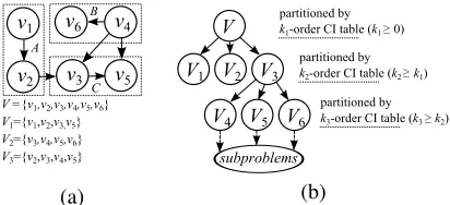
Example 1.Fig. 2(a) is an example to illustrate the pro-cess of Alg. 2. The input set V={v1, ...,v6} is partitioned
by 1-order CI tableM (as 0-order CI table is not enough
to partitionV, we therefore need to construct the 1-order CI table), we haveV={A={v1,v2},B={v4,v6},C={v3,v5}}. As M31=1 and M36=1, we further obtain V1={v1,v2,v3,v5}, V2={v3,v4,v5,v6} and V3={v2,v3,v4,v5}. We can see that ∀vi,vj∈V, ifviandvjare non-adjacent, then they are split
into different subsets, or they ared-separable in at least one subsetV1orV2orV3, i.e., thed-separation holds.
Example 2. On the other hand, as Alg. 2 is a subroutine of CAPA (Alg. 1), here we give an example in Fig. 2(b) to illustrate the whole process of finding causal partitionings by CAPA. The original variable setVis partitioned into three subsets{V1,V2,V3}based on thek1-order (k1≥0) CI table
regardingV. SupposeV1andV2cannot be further partitioned,
we terminate the recursive partitioning process onV1andV2.
AndV3will be further partitioned intoV4,V5andV6based on
thek2-order (k2≥k1) CI table regardingV3. Such a process
continues till all subsets meet the termination condition.
v1
v2 v3 v5 v4 v6
V ={v1,v2,v3,v4,v5,v6} V1={v1,v2,v3,v5} V2={v3,v4,v5,v6} V3={v2,v3,v4,v5}
A B
C
(a)
V
V2 V3
subproblems partitioned by
k1-order CI table (k1 0)
partitioned by
k2-order CI table (k2 k1)
partitioned by
k3-order CI table (k3 k2)
V1
V5 V6
V4
(b)
Figure 2: (a) An example of finding causal partitioning by using Alg.2; (b) An example of finding causal partitionings by CAPA.
We can see that the partitioning process in CAPA consti-tutes a hierarchy, like a ternary tree. Child subsets are resulted from their parent subset by using the same or a higher-order CI table. Therefore, this partitioning scheme can reduce the
number of redundant CI tests as many as possible, and also generates more reliable results than the existing recursive methods such as SADA, as these methods use high-order CI tests in each iteration.
Distinguishing Markov Equivalence Classes
As aforementioned in Alg. 1, a specified causal learning algorithm Agwill be used to solve a subset if it cannot be
further partitioned by Alg. 2. In this subsection, we study how to distinguish Markov equivalence classes via ReCIT. Here, we first review the process of discoveringV-structures, which is the critical step for CI-based methods to determine causal directions. Consider a local structurex−z−y, ifxis independent ofygiven a set of variablesZ,x⊥y|Z, then we can infer thatx−z−yisx→z←yin casez<Z according
to the mechanism ofd-separation. But, ifz∈Z, we cannot draw any conclusion about the causal directions ofx−z−y
(before consistent propagation). Thus, the problem turns to how to orient directions in the case ofz ∈ Z. We have the following theorem:
Theorem 2 Given a variable set V generated by linear non-Gaussian additive noise model. For any subset of V and its corresponding subgraph satisfying the faithfulness condition, and containing two random variables x and y as well as a set of other variables Z, if x (or y) is adjacent to z (z∈ Z) and x−E(x|Z)⊥z (or y−E(y|Z)⊥z) holds, then z causes x (or z causes y).
Proof:Without loss of generality, we assumex−E(x|Z)⊥z. Letεdenote the exogenous disturbance ofz. Ifx−E(x|Z)6⊥ε,
then x−E(x|Z)6⊥z according to Darmois-Skitovitch theo-rem (Darmois 1953; Skitovich 1953). We therefore have
x−E(x|Z)⊥ε, which means xandεcan bed-separated by
Zunder the faithfulness condition. Ifzis a child ofx, then
x→z←εforms aV-structure wherezis a collider, then there must bex−E(x|Z)6⊥ εor faithfulness is violated. This is a contradiction. Therefore, z can only be the parent of x. Similarly, we can prove the case w.r.t.y.
According to the process of causal partitioning, the (lo-cal) structure similar tox→z→y,x←z←yandx←z→ywill be preserved in at least one subset. Therefore, the depen-dence betweenx−E(x|Z) andzcan be used for determining directions (Line 3, Alg. 1).
Theoretical Analysis
In this section, we study the properties of CAPA, including correctness, completeness and complexity.
Correctness and completeness.We have the following the-orem:
Theorem 3 Given a variable set V={v1, ...,vn}following a
causal graph G. If all CI tests performed in CAPA are reliable, then CAPA returns the actual graph G.
Proof: Let G0 denote the causal graph reconstructed by
CAPA. The correctness and completeness are equivalent to the propositions:
1. Completeness:∀(v1→v2)∈G⇒(v1→v2)∈G0;
As discussed in Theorem 1, the causal partitioning returned by Alg. 2 in each iteration is theoretically valid. Assume that
Vis first partitioned into (V1,V2,V3), and the three subsets
cannot be further partitioned. According to the Condition 2 in Def. 1, we know that any adjacent variables cannot be separated during partitioning, the completeness is therefore guaranteed. On the other hand, because of the Condition 3 in Def. 1, any non-adjacent variable is either separated during partitioning ord-separable in at least one subset, i.e., the correctness is satisfied.
Therefore, the question turns to that ifV1(orV2,V3) can
be further partitioned, can CAPA still meet the complete-ness and correctcomplete-ness? We present the following proposi-tion:If two groups of variable sets S1={V1,...,Vt,...,Vm}and
S2={Vt1,...,Vtk}are two causal partitionings over V and Vt respectively, then S2∪S1\Vtforms a causal partitioning over V.The proof of this proposition is straightforward according to Definition 1. It implies that no matter how many times a set is partitioned by CAPA, if the returned causal partitioning in each iteration is valid, then all the resulting partitionings con-stitute an whole valid partitioning. Thus, as aforementioned, CAPA meets the completeness and correctness.
Time complexity.We focus on the number of CI tests used in CAPA since the other operations are computationally negli-gible compared to CI tests. Suppose that the original variable set V={v1, ...,vn} is recursively partitioned into m subsets
{V1, ...,Vm}where|Vm| ≤nfor allm. Suppose that we use the
PC algorithm as the basic algorithm. Then the time complex-ity of solving subproblems isO(mk2
max2kmax−2), wherekmax=
max(|V1|, ...,|Vm|). On the other hand, we need to calculate
a CI table in each iteration. In the worst case, we have to calculate aσ-order CI table w.r.t. the original variable set
V. Therefore, the upper bound of time complexity of CAPA isO(mk2
max2kmax−2+nσ+2). In practice, the step of dividing
a set into three non-overlapping subsets (Line 4 in Alg. 2) may consume considerable time if the causal structure is very large or complex. We have three strategies to accelerate CAPA: 1) using aσ-order CI table in the first time instead of using ones from 0 toσ-order, 2) terminating the causal par-titioning process when the current subset is sufficient small, and 3) employing a faster CI testing method such as partial correlation with Fisher transformation (Cai, Zhang, and Hao 2017) to check CI. If CI holds, we further use ReCIT to orient causal directions.
Performance Evaluation
We first compare CAPA with one of the latest recursive learn-ing methods SADA (Cai, Zhang, and Hao 2017) by extensive simulated experiments for evaluating their abilities of find-ing causal partitionfind-ing and learnfind-ing causal directions. To further illustrate the advantage of CAPA in causal structure learning, we also compare CAPA with four other existing causal learning methods, including LiNGAM (Shimizu et al. 2006), DLiNGAM (Shimizu et al. 2011), Sparse-ICA LiNGAM (Zhang et al. 2009) and SADA-LiNGAM (Cai, Zhang, and Hao 2017), over various real-world causal struc-tures. Note that all these four methods can distinguish Markov equivalence classes, in which SADA-LiNGAM stands for the state of the art in high-dimensional cases.
Performance on simulated structures. In this group of ex-periments, we evaluate our method on datasets generated by simulated causal network structures, under the linear non-Gaussian model. Because there are not large-scale causal inference problems with ground truth, simulated data on synthetic and real-world structures are used in most causal structure learning methods (Kalisch and B¨uhlmann 2007). The structures and data generating processes are similar to those presented in (Cai, Zhang, and Hao 2017). Concretely, we first randomly generate a set of root nodes, then itera-tively generate descendants in two steps: 1) Randomly select a subset of nodes from the generated nodes; 2) Using the selected nodes as parent nodes to generate a descendant with the average in-degree being 1.5. We then generate the data ac-cording to the corresponding structures with a linear function asvi=Pvj∈Paviwi jvj+εi, wherePavi denotes the parents ofvi andεiis the non-Gaussian noise term. When generating these
linear functions, we letP
Paviwi j=1 and the varianceVarεi=1
for every variablevi. To save time, we terminate the causal
partitioning process when the regarding subset is smaller than
|V|/10 and limit the maximum size of controlling set at 3.
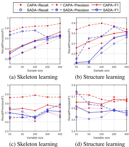
We first compare CAPA with SADA over the above sim-ulated models with different sample sizes{25, 50, 100, 200,
400}and 100 nodes. Both CAPA and SADA use PC
algo-rithm (Spirtes, Glymour, and Scheines 2000) as their basic algorithm for causality discovery from the partitioned subsets. The results are shown in Fig. 3(a) and (b).
25 50 100 200 400
Sample size
0.2 0.4 0.6 0.8 1
Recall/Precision/F1
(a) Skeleton learning
25 50 100 200 400
Sample size
0 0.2 0.4 0.6 0.8
Recall/Precision/F1
(b) Structure learning
25 50 100 200 400
Variable size
0.5 0.6 0.7 0.8 0.9 1
Recall/Precision/F1
(c) Skeleton learning
25 50 100 200 400
Variable size
0.4 0.5 0.6 0.7 0.8
Recall/Precision/F1
(d) Structure learning
From Fig. 3(a), we can see that CAPA performs better
than SADA in terms of precisionandF1 on causal
skele-ton learning for different sample sizes. The reason is that
d-separation is violated in SADA, thus many non-adjacent variables cannot be separated by the base solver. However, therecallscore of SADA is slightly better than that of CAPA. This is the result of two counteracting factors: 1)d-separation is preserved in CAPA, thus there are some subsets that can no longer be partitioned by CAPA, but can be still partitioned by SADA. That is, the CI tests regarding some adjacent variables in these ‘larger’ subsets are easier to fall into Type II error. 2) In SADA, the variable set is divided by using normal order CI tests, while in CAPA, the variable set is partitioned the σ-order CI table. Moreover, CAPA uses much fewer CI tests than SADA. Therefore, as the size of variable set increases, CI testing between two variables in SADA becomes easier and easier to fall into Type II error.
We also evaluate our method on causal structure learn-ing (with direction orientation), and the results are shown in Fig. 3(b). CAPA performs much better than SADA in terms ofRecall,PrecisionandF1. This is because CAPA can learn more causal directions byx−E(x|Z)⊥z(ory−E(y|Z)⊥z) ac-cording to Theorem 2, while SADA orients directions based on only V-structure learning and consistent propagation.
We then compare CAPA with SADA over different
dimen-sional networks{25, 50, 100, 200, 400}with 400 samples. The results are presented in Fig. 3(c) and (d), which show that the performance of CAPA and SADA for different variable sizes is relatively stable on both skeleton and structure learn-ing. We can conclude that the two methods are able to solve relatively higher dimensional problems over these simulated networks. However, real-world causal structures are more complex, and the dimensionality will impact the performance of the two methods, which will be further discussed later.
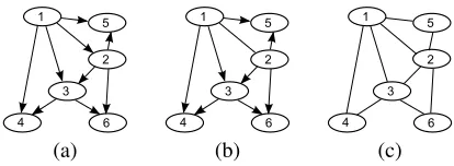
Performance of distinguishing equivalence classes.To fur-ther illustrate the advantage of CAPA in inferring causal di-rections, here we apply CAPA to a causal graph presented in (Shimizu et al. 2006), which was generated by following linear non-Gaussian structure equation model w.r.t. a DAG consisting of six variables as shown in Fig. 4(a). The graphs reconstructed by CAPA and SADA are shown in Fig. 4(b) and (c), respectively. We can see that all the causal direc-tions discovered by CAPA are correct, because CAPA can infer (v1,v3)→v4according tov4−E(v4|v1,v3)⊥(v1,v3).
Simi-larly, (v1,v2)→(v3,v5) and (v2,v3)→v6can also be obtained
by CAPA. There is only one edgev1−v2that is not oriented.
On the other hand, as shown in Fig. 4(c), though the skele-ton is correct, the corresponding directions are not inferred by any propagation. Because there is noV-structure in this graph, theoretically SADA cannot find any causal direction.
Performance on real-world structures
In this subsection, we compare CAPA with four other existing causal structure learning methods, including LiNGAM (Shimizu et al. 2006), DLiNGAM (Shimizu et al. 2011), Sparse-ICA LiNGAM (Zhang et al. 2009) and SADA-LiNGAM (Cai, Zhang, and Hao 2017). As all these methods can break Markov equivalence classes, we there-fore can further evaluate the performance of our method in
1
3 2 5
4 6
(a)
1
3 2 5
4 6
(b)
1
3 2 5
4 6
(c)
Figure 4: Performance comparison in causal direction in-ference. (a) The ground truth causal model; (b) The DAG reconstructed by CAPA; (c) The PDAG reconstructed by SADA.
.
causal structure learning. The implementations of LiNGAM, DLiNGAM and SADA-LiNGAM strictly follow the cor-responding original papers (Shimizu et al. 2006; 2011; Cai, Zhang, and Hao 2017). The implementation of Sparse-ICA LiNGAM is based on the sparse-Sparse-ICA of (Zhang et al. 2009) and the pruning algorithm of (Shimizu et al. 2006). Among these existing methods, SADA-LiNGAM is the most effective approach for learning causal structures of high dimensional cases, where LiNGAM is selected as the base solver by default. All methods are evaluated on eight real-world causal network structures1 that cover a variety
of applications, including insurance evaluation (Insurance), medicine (Alarm and Pathfinder), agricultural industry ( Bar-ley), weather forecasting (Hailfinder), system troubleshoot-ing (Win95pts and Andes) and the pedigree of breeding pigs (Pigs). Table 1 gives the structural statistics of these causal networks.
Note that the performance of the four counterparts is highly influenced by the ratio of the sample size to the number of nodes (Cai, Zhang, and Hao 2017), and the baseline approach LiNGAM is usually unreliable when the number of samples is less than 2|V|. We therefore compare CAPA against the four existing methods by fixing the sample size to 2|V|in the following experiments.
Table 1: Statistics of the eight causal network structures.
Dataset Nodes# Avg. degree Max degree
Insurance 27 3.95 9
Alarm 37 2.49 6
Barley 48 3.50 8
Hail f inder 56 2.36 17
Win95pts 76 1.84 9
Path f inder 109 3.58 106
Andes 223 3.03 12
Pigs 441 2.68 41
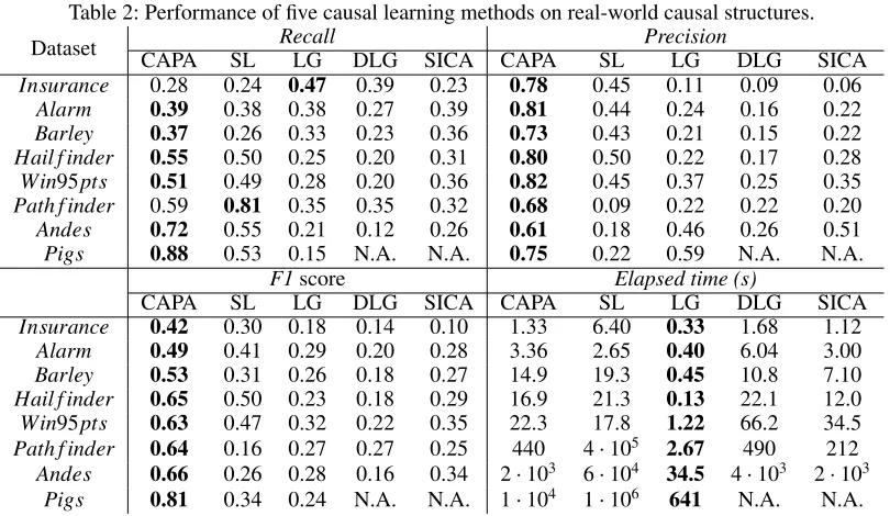
The results are shown in Table 2, where for compress-ing the space in the table, SADA-LiNGAM, LiNGAM, DLiNGAM and Sparse-ICA LiNGAM are simply denoted as SL, LG, DLG and SICA, respectively. It can be seen that CAPA achieves significantly betterprecisionandF1score on all structures. Only in the case ofInsuranceLiNGAM works
Table 2: Performance of five causal learning methods on real-world causal structures.
Dataset Recall Precision
CAPA SL LG DLG SICA CAPA SL LG DLG SICA
Insurance 0.28 0.24 0.47 0.39 0.23 0.78 0.45 0.11 0.09 0.06
Alarm 0.39 0.38 0.38 0.27 0.39 0.81 0.44 0.24 0.16 0.22
Barley 0.37 0.26 0.33 0.23 0.36 0.73 0.43 0.21 0.15 0.22
Hail f inder 0.55 0.50 0.25 0.20 0.31 0.80 0.50 0.22 0.17 0.28
Win95pts 0.51 0.49 0.28 0.20 0.36 0.82 0.45 0.37 0.25 0.35
Path f inder 0.59 0.81 0.35 0.35 0.32 0.68 0.09 0.22 0.22 0.20
Andes 0.72 0.55 0.21 0.12 0.26 0.61 0.18 0.46 0.26 0.51
Pigs 0.88 0.53 0.15 N.A. N.A. 0.75 0.22 0.59 N.A. N.A.
F1score Elapsed time (s)
CAPA SL LG DLG SICA CAPA SL LG DLG SICA
Insurance 0.42 0.30 0.18 0.14 0.10 1.33 6.40 0.33 1.68 1.12
Alarm 0.49 0.41 0.29 0.20 0.28 3.36 2.65 0.40 6.04 3.00
Barley 0.53 0.31 0.26 0.18 0.27 14.9 19.3 0.45 10.8 7.10
Hail f inder 0.65 0.50 0.23 0.18 0.29 16.9 21.3 0.13 22.1 12.0
Win95pts 0.63 0.47 0.32 0.22 0.35 22.3 17.8 1.22 66.2 34.5
Path f inder 0.64 0.16 0.27 0.27 0.25 440 4·105 2.67 490 212
Andes 0.66 0.26 0.28 0.16 0.34 2·103 6·104 34.5 4·103 2·103
Pigs 0.81 0.34 0.24 N.A. N.A. 1·104 1·106 641 N.A. N.A.
better than CAPA and in the case of Path f inder
SADA-LiNGAM works better than CAPA, all in terms ofRecall
score. In most cases, especially in larger causal networks
(with|V| > 100), CAPA works much better than
SADA-LiNGAM. The other three methods, LiNGAM, DLiNGAM and Sparse-ICA LiNGAM are not competitive in all these cases in terms of learning accuracy. As DLiNGAM and Sparse-ICA LiNGAM are of high time-complexity, here we do not present their results on thePigsnetwork.
In summary, we have the following observations:
1. The performance (Recall,Precision and F1 score) of CAPA turns better with the increase of the sample size, rather than the ratio of the sample size to the number of nodes (2|V|), while the performance of the four existing methods work more stable with a fixed ratio of the sample size to the number of nodes (2|V|). We can also see that on larger networks,Path f inder,AndesandPigs, theF1
score of CAPA is from 2 to 3 times higher than that of the four existing methods. Therefore, CAPA is more effective in causal discovery in high-dimensional cases in terms of inference accuracy when limited samples are given.
2. As the dimensionality of causal networks increases, the ratio ofRecalltoPrecisionof CAPA remains relatively stable, therefore theF1score of CAPA maintains at an acceptable level. On the contrary, we can see that on
small causal networks,Precisionof SADA-LiNGAM is
slightly higher thanRecall, while in the cases of larger causal networks, likePath f inderandAndes,Precision
of SADA-LiNGAM is much lower thanRecall. Note that
Recall is the fraction of actual causality found by the algorithm, andPrecisionis the actual fraction of inferred causality with respect to the true graph. We can say that SADA-LiNGAM cannot remove many incorrect causal relationships in these networks. On the other hand, CAPA
does particularly well in all these networks in terms of
precision.
3. By comparing the time costs of CAPA and SADA-LiNGAM, we notice that the time cost of CAPA increases with the size of variables, while the efficiency of SADA-LiNGAM is not stable. The reason is that in the step of finding causal partitioning, CAPA determines a smallerC
set by solving an optimization problem (Line 4 in Alg. 2),
while SADA-LiNGAM chooses aCset randomly.
Gen-erally, the smallerC, the higher accuracy and the less running time (Cai, Zhang, and Hao 2017). So we can con-clude that CAPA is more applicable to causal discovery in high-dimensional cases than these existing methods.
Conclusion
Acknowledgement: This work was supported by NSFC under gant No. U1636205. Jihong Guan and Xin Wang were supported by NSFC under grants No. 61772367 and No. 61772420, respectively.
References
Bergsma, W. P. 2004. Testing conditional independence for continuous random variables. Eurandom.
Cai, R.; Zhang, Z.; and Hao, Z. 2013. Causal gene identifica-tion using combinatorial v-structure search.Neural Networks
43:63–71.
Cai, R.; Zhang, Z.; and Hao, Z. 2017. SADA: A general framework to support robust causation discovery with theo-retical guarantee.CoRRabs/1707.01283.
Chickering, D. M. 2002. Learning equivalence classes of bayesian-network structures. The Journal of Machine Learn-ing Research2:445–498.
Darmois, G. 1953. Analyse g´en´erale des liaisons stochas-tiques: etude particuli`ere de l’analyse factorielle lin´eaire. Re-vue de l’Institut international de statistique2–8.
Doran, G.; Muandet, K.; Zhang, K.; and Sch¨olkopf, B. 2014. A permutation-based kernel conditional independence test.
Edwards, D. 2012. Introduction to graphical modelling.
Springer Science & Business Media.
Flaxman, S. R.; Neill, D. B.; and Smola, A. J. 2016. Gaussian processes for independence tests with non-iid data in causal
inference. ACM TIST7(2):22–1.
Fukumizu, K.; Gretton, A.; Sun, X.; and Sch¨olkopf, B. 2007.
Kernel measures of conditional dependence. Advances in
Neural Information Processing Systems20(1):167–204.
Gao, T., and Ji, Q. 2015. Local causal discovery of direct causes and effects. InAdvances in Neural Information Pro-cessing Systems, 2512–2520.
Geng, Z.; Wang, C.; and Zhao, Q. 2005. Decomposition of search for v-structures in DAGs. Journal of Multivariate Analysis96(2):282–294.
Grosse-Wentrup, M.; Janzing, D.; Siegel, M.; and Sch¨olkopf, B. 2016. Identification of causal relations in neuroimag-ing data with latent confounders: An instrumental variable
approach.NeuroImage125:825–833.
Kalisch, M., and B¨uhlmann, P. 2007. Estimating high-dimensional directed acyclic graphs with the pc-algorithm.
Journal of Machine Learning Research8(Mar):613–636. Koller, D., and Friedman, N. 2009.Probabilistic graphical models: principles and techniques. MIT press.
Liu, H.; Zhou, S.; Lam, W.; and Guan, J. 2017. A new hybrid method for learning bayesian networks: Separation
and reunion.Knowledge-Based Systems121:185 – 197.
Pearl, J. 2009.Causality. Cambridge university press.
Peters, J.; Janzing, D.; and Sch¨olkopf, B. 2011. Causal in-ference on discrete data using additive noise models.Pattern Analysis and Machine Intelligence, IEEE Transactions on
33(12):2436–2450.
Ramsey, J. D. 2014. A scalable conditional
indepen-dence test for nonlinear, non-gaussian data. arXiv preprint arXiv:1401.5031.
Shimizu, S.; Hoyer, P. O.; Hyv¨arinen, A.; and Kerminen, A. 2006. A linear non-gaussian acyclic model for causal
dis-covery.The Journal of Machine Learning Research7:2003–
2030.
Shimizu, S.; Inazumi, T.; Sogawa, Y.; Hyv¨arinen, A.; Kawa-hara, Y.; Washio, T.; Hoyer, P. O.; and Bollen, K. 2011. Directlingam: A direct method for learning a linear non-gaussian structural equation model. The Journal of Machine Learning Research12:1225–1248.
Skitovich, V. 1953. On a property of the normal distribution.
DAN SSSR89:217–219.
Spirtes, P.; Glymour, C. N.; and Scheines, R. 2000.Causation, prediction, and search, volume 81. MIT press.
Strobl, E. V.; Zhang, K.; and Visweswaran, S. 2017.
Approximate kernel-based conditional independence tests
for fast non-parametric causal discovery. arXiv preprint
arXiv:1702.03877.
Tian, J.; Pearl, J.; and Paz, A. 1998. Finding minimal d-separators.
Xie, X., and Geng, Z. 2008. A recursive method for structural
learning of directed acyclic graphs. Journal of Machine
Learning Research9(3):459–483.
Xie, X.; Geng, Z.; and Zhao, Q. 2006. Decomposition of structural learning about directed acyclic graphs. Artificial Intelligence170(4-5):422–439.
Zhang, K., and Hyv¨arinen, A. 2009. On the identifiability of the post-nonlinear causal model. InProceedings of the twenty-fifth conference on uncertainty in artificial intelligence, 647– 655. AUAI Press.
Zhang, K.; Peng, H.; Chan, L.; and Hyv¨arinen, A. 2009. Ica with sparse connections: Revisited. InInternational Confer-ence on Independent Component Analysis and Signal Sepa-ration, 195–202. Springer.
Zhang, K.; Peters, J.; Janzing, D.; and Sch¨olkopf, B. 2011. Kernel-based conditional independence test and application in causal discovery. 804–813. Corvallis, OR, USA: AUAI Press.