The Thirty-Third AAAI Conference on Artificial Intelligence (AAAI-19)
Sign-Full Random Projections
Ping Li
Cognitive Computing Lab (CCL) Baidu Research USA Bellevue, WA 98004, USA
Abstract
The method of 1-bit (“sign-sign”) random projections has been a popular tool for efficient search and machine learning on large datasets. Given twoD-dim data vectorsu,v∈RD, one can generatex=PD
i=1uiri, andy=
PD
i=1viri, where ri ∼ N(0,1) iid. Then one can estimate the cosine
simi-larityρfromsgn(x)andsgn(y). In this paper, we study a series of estimators for “sign-full” random projections. First
we proveE(sgn(x)y) =q2
πρ, which provides an
estima-tor forρ. Interestingly this estimator can be substantially im-proved by normalizing y. Then we study estimators based on E(y−1x≥0+y+1x<0) and its normalized version. We analyze the theoretical limit (using the MLE) and conclude that, among the proposed estimators, no single estimator can achieve (close to) the theoretical optimal asymptotic variance, for the entire range ofρ. On the other hand, the estimators can be combined to achieve the variance close to that of the MLE. In applications such as near neighbor search, duplicate detec-tion, knn-classificadetec-tion, etc, the training data are first trans-formed via random projections and then only the signs of the projected data points are stored (i.e., thesgn(x)). The origi-nal training data are discarded. When a new data point arrives, we apply random projections but we do not necessarily need to quantize the projected data (i.e., they) to 1-bit. Therefore, sign-full random projections can be practically useful. This gain essentially comes at no additional cost.
Introduction
Consider two high-dimensional data vectors, u, v ∈ RD.
Suppose we generate aD-dim random vector whose entries are iid standard normal, i.e.,ri∼N(0,1), and compute
x=
D
X
i=1
uiri, y=
D
X
i=1 viri
We have in expectation E(xy) = hu, vi = PD
i=1uivi.
If we generate x and y independently for k times, then
1
k
Pk
j=1xjyj ≈ E(xy) = hu, vi, and the quality of
ap-proximation improves as k increases. This idea of ran-dom projections has been widely used for large-scale search and machine learning (Johnson and Lindenstrauss 1984;
Copyright c2019, Association for the Advancement of Artificial Intelligence (www.aaai.org). All rights reserved.
Vempala 2004; Papadimitriou et al. 1998; Dasgupta 1999; Datar et al. 2004; Li, Hastie, and Church 2006).
A popular variant is the “1-bit” random projections (Goe-mans and Williamson 1995; Charikar 2002), which we refer to as “sign-sign” random projections, based on the following result of “collision probability”
P(sgn(x) =sgn(y)) = 1−cos
−1ρ
π (1)
whereρ=
PD i=1uivi
√
PD i=1u2i
√
PD i=1vi2
is the “cosine” similarity be-tween the two original data vectors u andv. The method of sign-sign random projections has become popular, for ex-ample, in many search related applications (Henzinger 2006; Manku, Jain, and Sarma 2007; Grimes 2008; Hajishirzi, Yih, and Kolcz 2010; T¨ure, Elsayed, and Lin 2011; Manzoor, Mi-lajerdi, and Akoglu 2016).
Note that by using only the signs of the projected data, we lose the information about the norms of the original vec-tors. Thus, in this context, with no loss of generality, we assume that the original data vectors are normalized, i.e.,
PD
i=1u 2
i =
PD
i=1v 2
i = 1. In other words, we can assume the projected data to bex∼N(0,1)andy∼N(0,1).
Interestingly, one can take advantage ofE(sgn(x)y)and several variants to considerably improve 1-bit random pro-jections. This gain essentially comes at no additional cost. Basically, the training data after projections are stored using signs (e.g.,sgn(x)). When a new data vector arrives, how-ever, we need to generate its random projections (y) but do not necessarily have to quantize them.
Related Work
The idea of “1-bit” projections has been extended to “sign cauchy projections” for estimatingχ2 similarity (Li,
Samorodnitsky, and Hopcroft 2013), and to “1-bit minwise hashing” (Broder 1997; Li and K¨onig 2010) for estimating the resemblance between sets. More general quantization schemes of random projections have been studied in, for ex-ample, (Li and Slawski 2017).
In the context of random projections, the idea of
estimat-ingρfromsgn(x)andywas explored in (Dong, Charikar,
Review of Estimators Based on Full Information
after Random Projections
In this context, since we are only concerned with estimating the cosineρ, we can without loss of generality assume that the original data are normalized, i.e.,kuk= kvk = 1. The projected data thus follow a bi-variant normal distribution:
xj
yj
∼N
0 0
,
1 ρ
ρ 1
, iid j = 1,2, ..., k.
whereρ=PD
i=1uivi. The obvious estimator forρis based on the inner product:
ˆ ρf =
1 k
k
X
j=1
xjyj, E( ˆρf) =ρ,
V ar( ˆρf) =
Vf
k , Vf = 1 +ρ
2
one can find the derivation of variance (i.e., Vf) in (Li, Hastie, and Church 2006). Note thatV ar( ˆρf)is the largest when|ρ|= 1. This is disappointing, because when two data vectors are identical, we ought to be able to estimate their similarity with no error. One can improve the estimator by simply normalizing the projected data. See (Anderson 2003) for the derivation.
ˆ ρf,n=
Pk
j=1xjyj
q Pk
j=1x 2
j
q Pk
j=1y 2
j
, E( ˆρf,n) =ρ+O
1
k
V ar( ˆρf,n) =
Vf,n
k +O
1
k2
, Vf,n= 1−ρ2
2
In particular, Vf,n = 0 when |ρ| = 1, as desired. One can further improveρˆf,n but not too much. The theoretical limit (i.e., the Cram´er-Rao bound) of the asymptotic vari-ance (Lehmann and Casella 1998) can be obtained by the maximum likelihood estimator (MLE), which is the solution of the following cubic equation:
ρ3−ρ2
k
X
j=1
xjyj+ρ
−1 +
k
X
i=1
x2j+ k
X
j=1
yj2
−
k
X
j=1
xjyj= 0
This cubic equation can have multiple real roots with a small probability (Li, Hastie, and Church 2006), which decreases exponentially fast with increasingk. The MLE is asymptot-ically unbiased and its asymptotic variance becomes:
E( ˆρf,m) =ρ+O
1
k
,
V ar( ˆρf,m) =
Vf,m
k +O
1
k2
, Vf,m=
1−ρ22
1 +ρ2
Estimator Based on Sign-Sign Random Projections
FromP r(sgn(xj) =sgn(yj)) = 1− 1πcos−1ρ, we have an asymptotically unbiased estimator and its variance:
ˆ
ρ1= cosπ
1−
1 k
k
X
j=1
1sgn(xj)=sgn(yj)
,
E( ˆρ1) =ρ+O
1
k
, V ar( ˆρ1) = V1
k +O
1
k2
,
V1= cos−1ρ π−cos−1ρ
(1−ρ2)
As later will be shown in Lemma 2, we have when|ρ| →1,
V1= 2√2π(1− |ρ|)3/2+o(1− |ρ|)3/2,
This rate is slower than O (1− |ρ|)2
, which is the rate at which Vf,n and Vf,m approach 0. Figure 1 compares the estimators in terms of V1
Vf,m,
Vf
Vf,m, and
Vf,n
Vf,m. Basically,
Vf,n < Vf always which means we should always use the
normalized estimator. Note thatV1< Vf if|ρ|>0.5902.
-1
-0.5
0
0.5
1
1
2
3
4
5
6
Var Ratios
V
mV
f
V
f,n
V
1Figure 1: Ratios (lower the better) of variance factors: V1
Vf,m,
Vf
Vf,m,
Vm
Vf,m,
Vf,n
Vf,m. They are always larger than 1, asVf,mis
the theoretically smallest variance factor. Note thatVmis the variance factor for the MLE of sign-full random projections.
Estimators for Sign-Full Random Projections
In many practical scenarios such as near-neighbor search and near-neighbor classification, we can store signs of the projected data (i.e.,sgn(xj)) and discard the original high-dimensional data. When a new data vector arrives, we gen-erate its projected vector (i.e.,y). At this point we actually have the option to choose whether we would like to use the full information or just the signs (i.e.,sgn(yj)) to estimate the similarityρ. If we are able to find a better (more accu-rate) estimator by using the full information ofyj, there is no reason why we have to only use the sign ofyj.We first study the maximum likelihood estimator (MLE), in order to understand the theoretical limit.
Theorem 1 Given k iid samples (sign(xj), yj), j =
1,2, ..., k, withxj, yj ∼ N(0,1),E(xjyj) = ρ, the
max-imum likelihood estimator (MLE, denoted byρˆm) is the
so-lution to the following equation:
k
X
j=1 φ
ρ √
1−ρ2sgn(xj)yj
Φ
ρ √
1−ρ2sgn(xj)yj
sgn(xj)yj= 0 (2)
φ(t) = √1 2πe
−t2/2
andΦ(t) =Rt
−∞φ(t)dtare respectively
E( ˆρm) =ρ+O
1 k
, V ar( ˆρm) =
Vm
k +O
1 k2
,
1 Vm
=E
ρ (1−ρ2)7/2
φ
ρ
√
1−ρ2sgn(xj)yj
Φ
ρ
√
1−ρ2sgn(xj)yj
sgn(xj)y 3
j
+E
1 (1−ρ2)3
φ2
ρ
√
1−ρ2sgn(xj)yj
Φ2
ρ
√
1−ρ2sgn(xj)yj
y 2
j
(3)
−E
3ρ (1−ρ2)5/2
φ
ρ
√
1−ρ2sgn(xj)yj
Φ
ρ
√
1−ρ2sgn(xj)yj
sgn(xj)yj
.
As the MLE equation (2) is quite sophisticated, we study this estimator mainly for theoretical interest, for example, for evaluating other estimators. We can evaluate the expec-tations in (3) by simulations. Figure 1 already plots Vm
Vf,m, to
compareρˆmwith three estimators:ρ1ˆ ,ρˆf,ρˆf,n. The figure shows thatρˆmindeed substantially improvesρ1ˆ .
Next, we seek estimators which are much simpler than
ˆ
ρm. Ideally, we look for estimators which can be written as “inner products”. In this paper, we studyfoursuch estima-tors. We first present a Lemma which will be needed for de-riving these estimators and proving their properties. The re-sults can also be easily validated by numerical integrations. Lemma 1
Z ∞
0
te−t2/2Φ p ρt 1−ρ2
!
dt= 1 +ρ
2 (4)
Z ∞
0
t3e−t2/2Φ p ρt 1−ρ2
!
dt=1
2 2 + 3ρ−ρ
3
(5)
Z ∞
0
t2e−t2/2Φ p ρt 1−ρ2
!
dt (6)
= 1ρ≥0
r
π
2 −
r
1
2π tan
−1
p
1−ρ2
ρ −ρ
p
1−ρ2
!
where we denote thattan−1 1
0
= tan−1 1
0+
=π
2.
The first estimator we present is based on the (odd) mo-ments of(sgn(xj)yj)as shown in Theorem 2.
Theorem 2
E(sgn(xj)yj) =
r
2
πρ, (7)
E (sgn(xj)yj)3
= √1
2π 6ρ−2ρ
3
(8)
Proof Sketch: Note that: E (sgn(xj)2yj)2
= 1, and E (sgn(xj)yj)4= 3. Because(xj, xj)is bi-variate
nor-mal, we havexj|yj∼N ρyj, (1−ρ2)
, and
E(sgn(xj)yj)) =E(yjE(sgn(xj)|yj))
=E(yjP r(xj|yj≥0)−yjP r(xj|yj<0))
=E yj 1−2Φ
−ρyj
p
1−ρ2
!!!
=E yj 2Φ
ρyj
p
1−ρ2
! −1
!!
=2
Z ∞
−∞
tφ(t)Φ p ρt
1−ρ2
!
dt
=4
Z ∞
0
tφ(t)Φ p ρt
1−ρ2
!
dt−2
Z ∞
0
tφ(t)dt
=41 +ρ
2 1
√
2π−2
1
√
2π =
r
2
πρ, result in Lemma 1
Similarly, using result from Lemma 1
E sgn(xj)y3j)
= 4
Z ∞
0
t3φ(t)Φ p ρt
1−ρ2
!
dt
−2
Z ∞
0
t3φ(t)dt=√1
2π 6ρ−2ρ
3
.
Theorem 2 leads to a simple estimatorρˆgand its variance:
ˆ ρg =
1 k
k
X
j=1
r
π
2sgn(xj)yj, E( ˆρg) =ρ (9)
V ar( ˆρg) =
Vg
k , Vg=
π
2 −ρ
2 (10)
The variance does not vanish when|ρ| → 1. Interestingly, the variance can be substantially reduced by applying a nor-malization step onyj, as shown in Theorem 3.
Theorem 3 Ask→ ∞, the following asymptotic normality holds:
√
k
r
π 2
Pk
j=1sgn(xj)yj √
k
q Pk
j=1y 2
j −ρ
D
=⇒N(0, Vg,n) (11)
Vg,n=Vg−ρ2 3/2−ρ2
(12)
whereVg=π2 −ρ2as in (10).
Proof Sketch: LetZk =
Pk
j=1sgn(xj)yj √
kqPk j=1y2j
. Ask→ ∞, then
1 k
k
X
j=1
y2j →E y2j
= 1, a.s.
Zk =
1
k
Pk
j=1sgn(xj)yj
q
1
kk
q
1
k
Pk
j=1y2j →
r
2
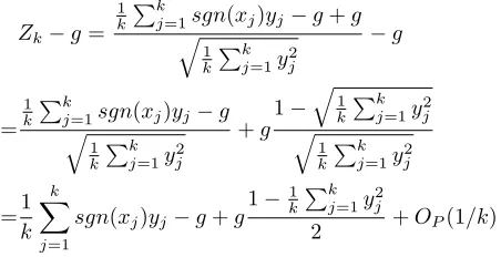
We express the deviationZk−gas
Zk−g=
1
k
Pk
j=1sgn(xj)yj−g+g
q
1
k
Pk
j=1yj2
−g
= 1
k
Pk
j=1sgn(xj)yj−g
q
1
k
Pk
j=1y2j
+g
1−q1
k
Pk
j=1y 2
j
q
1
k
Pk
j=1yj2
=1
k
k
X
j=1
sgn(xj)yj−g+g
1−1
k
Pk
j=1y 2
j
2 +OP(1/k)
Thus, to analyze the asymptotic variance, it suffices to study:
E
sgn(x)y−g+g1−y
2
2
2
=E sgn(x)y−g(1 +y2)/22
=E(y2) +g2E(1 +y4+ 2y2)/4−gE(sgn(x)(y+y3))
=1 +g2(1 + 3 + 2)/4−gE(sgn(x)(y+y3))
=1 + 3/2g2−g2−gg3= 1−1
π 5ρ
2−2ρ4
where we recallg3=E sgn(x)y3)=√1
2π 6ρ−2ρ
3
.
Theorem 3 leads to the following estimatorρˆg,n:
ˆ ρg,n=
r
π 2
Pk
j=1sgn(xj)yj
√ k
q Pk
j=1yj2
, E( ˆρg,n) =ρ+O
1
k
,
V ar( ˆρg,n) =
Vg,n
k +O
1 k2
This normalization always helps, becauseVg,n≤Vg. We can develop more estimators based on Theorem 4.
Theorem 4
E(y−1x<0+y+1x≥0) =
1 +ρ
√
2π (13)
E(y−1x<0+y+1x≥0)2 (14)
= 1ρ≥0− 1
π tan
−1
p
1−ρ2 ρ
!
−ρp1−ρ2
!
E(y−1x≥0+y+1x<0) =
1−ρ
√
2π (15)
E(y−1x≥0+y+1x<0)
2
(16)
= 1ρ<0+ 1
π tan
−1
p
1−ρ2 ρ
!
−ρp1−ρ2
!
This leads to another estimator, denoted byρˆs:
ˆ
ρs= 1−
√
2π k
k
X
j=1
yj−1xj≥0+yj+1xj<0
(17)
E( ˆρs) =ρ, V ar( ˆρs) =
Vs
k
Vs= 2π×1ρ<0+ 2 tan−1
p
1−ρ2 ρ
!
(18)
−2ρp1−ρ2−(1−ρ)2
After a careful check, the estimator proposed in (Dong, Charikar, and Li 2008) is equivalent to ρˆs, despite the different expressions. (Dong, Charikar, and Li 2008) used hyper-spherical projection which is equivalent to random projection for high-dimensional original data. The variance expression in (Dong, Charikar, and Li 2008) appeared different but it is indeed the same as the variance ofρˆsif we let original data dimension be large.
We can again try to normalize the projected data for the hope of obtaining an improved estimator:
Theorem 5 √
k
Pk
j=1yj−1xj≥0+yj+1xj<0
√
k
q Pk
j=1y 2
j
−1√−ρ
2π
(19)
D
=⇒N(0, Vs,n)
Vs,n=Vs−
(1−ρ)2
4π 1−2ρ−2ρ
2
(20)
whereVsis in (18). .
This leads to the following estimator:
ˆ
ρs,n= 1−
Pk
j=1
√
2π
yj−1xj≥0+yj+1xj<0
√
kqPk
j=1y 2
j
(21)
E( ˆρs,n) =ρ+O
1 k
, V ar( ˆρs,n) =
Vs,n
k +O
1 k2
whereVs,nis in (20). The resultant estimatorρˆs,n has the property that the variance approaches 0 as ρ → 1. The normalization step however does not always help. From (20), we haveVs ≥ Vs,nifρ ≤
√ 3−1
2 ≈ 0.3660. On the
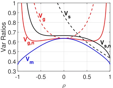
other hand, as shown in Figure 2, the normalization step only increases the variance slightly ifρ >0.3660.
Figure 2 plots the rations:Vm
V1,
Vg
V1,
Vg,n
V1 ,
Vs
V1,
Vs,n
V1 , to
com-pare those five estimators in terms of their improvements relative to the 1-bit estimatorρ1ˆ . As expected, the MLEρˆm achieves the smallest asymptotic variance and Vm
V1 = 2
π at
ρ = 0and Vm
V1 ≈0.36at|ρ| →1. This means in the high
similarity region, usingρˆmcan roughly reduce the required number of samples (k) by a factor of 3. Overall,ρˆs,nis com-putationally simple and its variance is very close to the vari-ance of the MLE, at least forρ≥ −0.4.
-1 -0.5 0 0.5 1 0.3
0.4 0.5 0.6 0.7 0.8 0.9 1
Var Ratios
V
g
V
g,n
Vs
V
s,n
V m
Figure 2: Variance ratios:Vm
V1,
Vg
V1,
Vg,n
V1 ,
Vs
V1,
Vs,n
V1 , to compare
the five estimators, in terms of the relative improvement with respect to the 1-bit estimatorρˆ1. The MLE (ρˆm, solid blue)
achieves the lowest asymptotic variance.
Lemma 2 Atρ= 0, Vm
V1
= Vg V1
=Vg,n V1
=2
π ≈0.6366, Vs
V1
= 4
π−
4
π2 ≈0.8680,
Vs,n
V1
= 4
π −
6
π2 ≈0.6653
As|ρ| →1,
V1= 2√2π(1− |ρ|)3/2+o(1− |ρ|)3/2 (22)
Asρ→1,
Vs
V1 =
Vs,n
V1 =
4
3π ≈0.4244,
Vg
V1 =∞,
Vg,n
V1 =∞
Recommendation for Estimators
We have studied four estimators (with closed forms) :ˆ ρg=
1 k
k
X
j=1
r
π
2sgn(xj)yj,
ˆ ρg,n=
r
π 2
Pk
j=1sgn(xj)yj √
k
q Pk
j=1y2j
,
ˆ
ρs= 1−
√
2π k
k
X
j=1
yj−1xj≥0+yj+1xj<0
,
ˆ
ρs,n= 1−
Pk
j=1
√
2πyj−1xj≥0+yj+1xj<0
√
k
q Pk
j=1y 2
j
The choice depends on application scenarios. Presumably, for a given query, we would like to retrieve data points which have similarityρclose to 1. However, for practical datasets, typically most data points are not similar at all. From Fig-ure 2, if we hope to use one single estimator, thenρˆs,nis the
overall best. We can also combine two estimators: ρˆsand
ˆ
ρg,n. Figure 2 showsρˆsis better ifρ >0.4437. Forρ < 0, we can always switch to the mirror version of the estimators.
A Simulation Study
We provide a simulation study to verify the theoretical prop-erties of the four estimators for sign-full random projections:
ˆ
ρg,ρˆg,n,ρˆs,ρˆs,n, as well asρˆ1for sign-sign projections.
For a givenρ, we simulatekstandard bi-variate normal variables (xj, yj)with E(xjyj) = ρ, j = 1, ..., k. Then we choose an estimator ρˆto estimate ρ. With 106
simu-lations, we plot the empirical mean square errors (MSEs):
M SE( ˆρ) = Bias2( ˆρ) +V ar( ˆρ), together with the
theo-retical variance of ρˆ. If the empirical MSE curve and the theoretical variance overlap, we know that the estimator is unbiased and the theoretical variance formula is verified.
10 100 1000
k 10-5
10-4 10-3
10-2 10-1
MSE
= 0.99 g
g,n
s s,n
10 100 1000
k 10-4
10-3 10-2 10-1
MSE
= 0.95
g
g,n
s s,n
10 100 1000
k
10-3
10-2
10-1
MSE
= 0.75
g
g,n
ss,n
10 100 1000
k
10-3
10-2
10-1
MSE
= 0
g g,n
s s,n
10 100 1000
k 10-4
10-3 10-2 10-1
MSE
= - 0.95
g
g,n s
s,n
10 100 1000
k 10-4
10-3 10-2 10-1
MSE
= - 0.99
g
g,n s
s,n
Figure 3: Empirical MSEs (solid curves) for four proposed estimators, together with theoretical (asymptotic) variances (dashed curves), for 6ρvalues. Forρˆgandρˆs, the solid and dashed curves overlap, confirming that they are unbiased and the variance formulas are correct. Forρˆg,nandρˆs,n, the solid and dashed curves overlap whenkis not too small.
Figure 3 presents the results for 6 selected ρ values:
0.99,0.95,0.75,0,−0.95,−0.99. Those simulations verify that bothρˆgandρˆsare unbiased, while their normalized ver-sionsρˆg,n andρˆs,n are asymptotically (i.e., whenk is not too small) unbiased. The (asymptotic) variance formulas for these four estimators are verified since the solid and dashed curves overlap (whenkis not small).
Figure 4 presents the ratios of empirical MSEs (solid curves): M SEM SE( ˆ( ˆρρ1)
s,n)and
M SE( ˆρ1)
theo-retical asymptotic variance ratios (dashed curves): V1
Vs,n and
V1
Vg,n. These curves again confirm the asymptotic variance
formulas. In addition, they indicate that in the high similarity region, when the sample sizekis not too large, the improved gained from usingρˆs,ncan be substantially more than what are predicted by theory. For example, whenρis close to 1 (e.g.,ρ= 0.99), theoretically V1
Vs,n = 3
4π≈2.3562, the
ac-tual improvement can be as much as a factor of 8 (atk= 10). This is the additional advantage ofρˆs,n.
10 100 1000
k 0
1 2 3 4 5 6 7 8
MSE Ratios
= 0.99
g,n s,n
10 100 1000
k 0
1 2 3 4 5
MSE Ratios
= 0.97
g,n s,n
10 100 1000
k 0
1 2 3 4
MSE Ratios
= 0.95
g,n s,n
10 100 1000
k 0
0.5 1 1.5 2 2.5
MSE Ratios
= 0.9
g,n s,n
Figure 4: Empirical rations: M SEM SE( ˆ( ˆρρs,n)1) and M SEM SE( ˆρ( ˆρg,n)1) , together with the theoretical asymptotic variance ratios (dashed curves): V1
Vs,n and
V1
Vg,n. When k is not small, the
solid and dashed curves overlap. At high similarity and small
k, the improvement would be even more substantial.
An Experimental Study
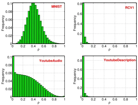
To further verify the theoretical results, we conduct an exper-imental study on the ranking task for near-neighbor search on 4 public datasets (see Table 1 and Figure 5).
Table 1: Information about the datasets Dataset # Train # Query # Dim
MNIST 10,000 10,000 780
RCV1 10,000 10,000 47,236
YoutubeAudio 10,000 11,930 2,000 YoutubeDescription 10,000 11,743 12,183,626
These four datasets are downloaded from either the UCI repository or the LIBSVM website. When a dataset contains significantly more than 10,000 training samples, we only use a random sample of it. The datasets represent a wide range of application scenarios and data types. See Figure 5 for the frequencies of all pairwiseρvalues.
For each data point in the query set, we estimate its sim-ilarity with every data point in the training set, using ran-dom projections. The goal is to return training data points with which the estimated similarities are larger than a pre-specified thresholdρ0. For each query point, we rank all the
0 0.2 0.4 0.6 0.8 1
0 0.02 0.04 0.06 0.08 0.1
ρ
Frequency
MNIST
0 0.2 0.4 0.6 0.8 1
0 0.2 0.4 0.6 0.8
ρ
Frequency
RCV1
0 0.2 0.4 0.6 0.8 1
0 0.02 0.04 0.06 0.08 0.1
ρ
Frequency
YoutubeAudio
0 0.2 0.4 0.6 0.8 1
0 0.2 0.4 0.6 0.8
ρ
Frequency
YoutubeDescription
Figure 5: Histograms of all pairwiseρvalues.
(estimated) similarities and return top-Lpoints. We can then compute the precision and recall
P recision=#retrieved points with true similarities ≥ρ0
L ,
Recall=#retrieved points with true similarities ≥ρ0 #total points with true similarities ≥ρ0
We report the averaged precision-recall values over all query data points. By varyingLfrom 1 to the number of training data points, we obtain a precision-recall curve.
Figure 6 presents the results for the RCV1 datasets, for
ρ0 ∈ {0.9,0.8,0.6}, and for k ∈ {50,100}. In the first row (i.e., ρ0 = 0.9), we can see that ρˆs,n is substantially more accurate than bothρˆ1andρˆg,n. Since this case
repre-sents the high-similarity region, as expected,ρˆg,nperforms poorly. For smaller ρ0 values,ρˆg,n performs substantially better, also as expected. Figure 7, Figure 8, and Figure 9 present the results for the other three datasets. The trends are pretty much similar to what we observe in Figure 6.
Conclusion
The method of sign-sign (1-bit) random projections has been a standard tool in practice. In many scenarios such as near-neighbor search and near-near-neighbor classification, we can store signs of the projected data and discard the original high-dimensional data. As a new data point arrives, one can generate its projected vector and use it (without taking signs) to estimate the similarity. We study various estimators for sign-full random projections and compare their variances with the theoretical limit. Nevertheless, a combination of two estimators (ρˆg,n andρˆs) can almost achieve the theo-retical bound. For applications which only allows a single estimator, the proposedρˆs,nis the overall best estimator.
References
Anderson, T. W. 2003. An Introduction to Multivariate
Sta-tistical Analysis. Hoboken, New Jersey: John Wiley & Sons,
0.5 0.6 0.7 0.8 0.9 1 0.82 0.84 0.86 0.88 0.9 0.92 Recall Precision RCV1
ρ0 = 0.9, k = 50
s,n
1
g,n
0.5 0.6 0.7 0.8 0.9 1
0.86 0.88 0.9 0.92 0.94 Recall Precision RCV1
ρ0 = 0.9, k = 100 s,n
1 g,n
0.4 0.5 0.6 0.7 0.8 0.9 1
0.65 0.7 0.75 0.8 0.85 0.9 Recall Precision RCV1
ρ0 = 0.8, k = 50 1 g,n s,n
0.4 0.5 0.6 0.7 0.8 0.9 1
0.78 0.8 0.82 0.84 0.86 0.88 0.9 0.92 0.94 Recall Precision RCV1 ρ
0 = 0.8, k = 100 1 g,n s,n
0.3 0.4 0.5 0.6 0.7 0.8 0.1 0.2 0.3 0.4 0.5 0.6 0.7 0.8 Recall Precision RCV1
ρ0 = 0.6, k = 50 1 g,n
s,n
0.3 0.4 0.5 0.6 0.7 0.8 0.9
0.55 0.6 0.65 0.7 0.75 0.8 0.85 Recall Precision RCV1 ρ
0 = 0.6, k = 100
1
g,n s,n
Figure 6:RCV1: precision-recall curves for selectedρ0and kvalues, and for three estimators:ρˆs,n,ρˆg,n,ρ1ˆ .
0.1 0.2 0.3 0.4 0.5 0.6 0.7 0.1 0.2 0.3 0.4 0.5 Recall Precision MNIST
ρ0 = 0.9, k = 50 1
g,n
s,n
0.1 0.2 0.3 0.4 0.5 0.6 0.7 0.2 0.3 0.4 0.5 0.6 0.7 Recall Precision MNIST ρ
0 = 0.9, k = 100 1 g,n s,n
0 0.2 0.4 0.6 0.8
0.1 0.2 0.3 0.4 0.5 0.6 Recall Precision MNIST ρ
0 = 0.8, k = 50 1
g,n s,n
0 0.2 0.4 0.6 0.8
0.3 0.4 0.5 0.6 0.7 0.8 Recall Precision MNIST ρ
0 = 0.8, k = 100
1
g,n s,n
0 0.2 0.4 0.6 0.8
0.2 0.4 0.6 0.8 1 Recall Precision MNIST ρ
0 = 0.6, k = 50 1
g,n s,n
0 0.2 0.4 0.6 0.8
0.4 0.5 0.6 0.7 0.8 0.9 1 Recall Precision MNIST ρ
0 = 0.6, k = 100 1
g,n s,n
Figure 7: MNIST: precision-recall curves for selectedρ0
andkvalues, and for three estimators:ρˆs,n,ρˆg,n,ρ1ˆ .
0.2 0.4 0.6 0.8
0.3 0.35 0.4 0.45 0.5 0.55 Recall Precision YoutubeAudio ρ
0 = 0.9, k = 50 1
g,n
s,n
0.2 0.4 0.6 0.8 0.4 0.45 0.5 0.55 0.6 0.65 0.7 0.75 Recall Precision YoutubeAudio ρ
0 = 0.9, k = 100 1
g,n
s,n
0.1 0.2 0.3 0.4 0.5 0.6 0.7 0.2 0.3 0.4 0.5 0.6 Recall Precision YoutubeAudio ρ
0 = 0.8, k = 50
1 g,n s,n
0.1 0.2 0.3 0.4 0.5 0.6 0.7 0.4 0.5 0.6 0.7 0.8 Recall Precision YoutubeAudio
ρ0 = 0.8, k = 100 1 g,n s,n
0 0.2 0.4 0.6 0.8
0.4 0.5 0.6 0.7 0.8 Recall Precision YoutubeAudio ρ
0 = 0.6, k = 50
1 g,n
s,n
0 0.2 0.4 0.6 0.8 0.5 0.6 0.7 0.8 0.9 Recall Precision YoutubeAudio
ρ0 = 0.6, k = 100 1
g,n
s,n
Figure 8: YoutubeAudio: precision-recall curves for se-lectedρ0andkvalues, and three estimators:ρˆs,n,ρˆg,n,ρ1ˆ .
0.6 0.7 0.8 0.9 1
0.91 0.92 0.93 0.94 0.95 0.96 0.97 Recall Precision ρ
0 = 0.9, k = 50
YoutubeDescription
s,n
g,n
1
0.6 0.7 0.8 0.9 1
0.94 0.95 0.96 0.97 0.98 0.99 Recall Precision ρ
0 = 0.9, k = 100
1 s,n
g,n YoutubeDescription
0.5 0.6 0.7 0.8 0.9 1 0.75 0.8 0.85 0.9 0.95 Recall Precision YoutubeDescription ρ
0 = 0.8, k = 50 1
g,n
s,n
0.6 0.7 0.8 0.9 1
0.9 0.91 0.92 0.93 0.94 0.95 0.96 Recall Precision ρ
0 = 0.8, k = 100 YoutubeDescription
s,n
g,n
1
0.4 0.6 0.8 1
0 0.2 0.4 0.6 0.8 1 Recall Precision YoutubeDescription
ρ0 = 0.6, k = 50 1 g,n s,n
0.5 0.6 0.7 0.8 0.9 1 0.65 0.7 0.75 0.8 0.85 0.9 Recall Precision YoutubeDescription ρ
0 = 0.6, k = 100 1 g,n
s,n
Broder, A. 1997. On the resemblance and containment of documents. InProceedings of the Compression and
Com-plexity of Sequences (Sequences), 21–29.
Charikar, M. 2002. Similarity estimation techniques from rounding algorithms. In Proceedings of the 34th Annual
ACM Symposium on Theory of Computing (STOC), 380–
388.
Dasgupta, S. 1999. Learning mixtures of gaussians. In
Proceedings of the 40th Annual Symposium on Foundations
of Computer Science (FOCS), 634–644.
Datar, M.; Immorlica, N.; Indyk, P.; and Mirrokni, V. S. 2004. Locality-sensitive hashing scheme based on p-stable distributions. InProceedings of the 20th ACM Symposium
on Computational Geometry (SoCG), 253–262.
Dong, W.; Charikar, M.; and Li, K. 2008. Asymmetric dis-tance estimation with sketches for similarity search in high-dimensional spaces. InProceedings of the 31st Annual In-ternational ACM SIGIR Conference on Research and
Devel-opment in Information Retrieval (SIGIR), 123–130.
Goemans, M. X., and Williamson, D. P. 1995. Improved approximation algorithms for maximum cut and satisfia-bility problems using semidefinite programming. J. ACM
42(6):1115–1145.
Gradshteyn, I. S., and Ryzhik, I. M. 1994.Table of Integrals,
Series, and Products. New York: Academic Press, fifth
edi-tion.
Grimes, C. 2008. Microscale evolution of web pages. In
Proceedings of the 17th International Conference on World
Wide Web (WWW), 1149–1150.
Hajishirzi, H.; Yih, W.-t.; and Kolcz, A. 2010. Adaptive near-duplicate detection via similarity learning. In Proceed-ings of the 33rd international ACM SIGIR conference on
Research and development in information retrieval (SIGIR),
419–426.
Henzinger, M. R. 2006. Finding near-duplicate web pages: a large-scale evaluation of algorithms. InSIGIR 2006: Pro-ceedings of the 29th Annual International ACM SIGIR Con-ference on Research and Development in Information
Re-trieval (SIGIR), 284–291.
J´egou, H.; Douze, M.; and Schmid, C. 2011. Product quan-tization for nearest neighbor search. IEEE Trans. Pattern
Anal. Mach. Intell.33(1):117–128.
Johnson, W. B., and Lindenstrauss, J. 1984. Extensions of Lipschitz mapping into Hilbert space. Contemporary
Math-ematics26:189–206.
Lehmann, E. L., and Casella, G. 1998. Theory of Point
Estimation. New York, NY: Springer, second edition.
Li, P., and K¨onig, A. C. 2010. b-bit minwise hashing. In
Proceedings of the 19th International Conference on World
Wide Web (WWW), 671–680.
Li, P., and Slawski, M. 2017. Simple strategies for recover-ing inner products from coarsely quantized random projec-tions. InAdvances in Neural Information Processing
Sys-tems (NIPS), 4570–4579.
Li, P.; Hastie, T.; and Church, K. W. 2006. Improving ran-dom projections using marginal information. InProceedings
of the 19th Annual Conference on Learning Theory (COLT),
635–649.
Li, P.; Samorodnitsky, G.; and Hopcroft, J. E. 2013. Sign cauchy projections and chi-square kernel. In Advances in
Neural Information Processing Systems (NIPS), 2571–2579.
Manku, G. S.; Jain, A.; and Sarma, A. D. 2007. Detecting near-duplicates for web crawling. InProceedings of the 16th
International Conference on World Wide Web (WWW), 141–
150.
Manzoor, E. A.; Milajerdi, S. M.; and Akoglu, L. 2016. Fast memory-efficient anomaly detection in streaming heteroge-neous graphs. InProceedings of the 22nd ACM SIGKDD In-ternational Conference on Knowledge Discovery and Data
Mining (KDD), 1035–1044.
Papadimitriou, C. H.; Raghavan, P.; Tamaki, H.; and Vem-pala, S. 1998. Latent semantic indexing: A probabilistic analysis. InProceedings of the Seventeenth ACM SIGACT-SIGMOD-SIGART Symposium on Principles of Database
Systems (PODS), 159–168.
T¨ure, F.; Elsayed, T.; and Lin, J. J. 2011. No free lunch: brute force vs. locality-sensitive hashing for cross-lingual pairwise similarity. InProceeding of the 34th International ACM SIGIR Conference on Research and Development in
Information Retrieval (SIGIR), 943–952.