Modelling 1-D signals using Hermite basis functions

(1)

MURDOCH RESEARCH REPOSITORY

http://dx.doi.org/10.1049/ip-vis:19971613

Rasiah, A.I., Togneri, R. and Attikiouzel, Y. (1997) Modelling 1-D

signals using Hermite basis functions. IEE Proceedings - Vision,

Image, and Signal Processing, 144 (6). pp. 345-354.

http://researchrepository.murdoch.edu.au/18660/

(2)

Modelling

1 -D signals using Hermite basis functions

A.I. Rasiah

R

.

Tog ne r i Y.Attikiouzel

Indexing terms: Hermite function, QRS detection, ECG analysis, Pattern recognition, Gaussian quadratures, LMS estimation

Abstract: The paper discusses a method for

estimating the Hermite coefficients of a discrete- time one-dimensional signal. To estimate the Hermite coefficients a solution based on Gaussian quadratures is used. The paper also looks at various least mean squared (LMS) estimation methods to estimate two further parameters which are incorporated into the orthonormal Hermite basis function; a spread term and a shift term. In addition, the effects of scaling, dilation and translates of a signal on its Hermite coefficients, spread and shift terms are presented. The paper concludes with a brief discussion on the potential application of the Hermite parameters as features for use in problems requiring shape discrimination within a one- dimensional signal. It also mentions those applications where this was found to be appropriate.

1 Introduction

The objective of any feature extraction process is to obtain a pattern space that retains sufficient information, has low dimensionality and provides good inter- class separation to enhance discrimination between the various feature classes.

A typical feature extraction process involves the parameterisation of a system in terms of a mathematical model and use of its parameters as features. In this paper, the model adopted for 1-D signal representation is a series expansion of N basis functions, where the features are the coefficients of these functions, and the pattern space is a space in

RN.

Using this model, com- parisons between the original signal and its synthesis (defined as the linear combination of basis functions) can easily be made. This provides a means to demonstrate the retention of relevant information by the features and, a way to determine the sufficiency of the number of features used.

0 IEE, 1997

IEE Proceedings online no. 19971613

Paper first received 17th July 1996 and in final revised form 25th Septem- ber 1997

A.I. Rasiah was with the University of Westem Australia and is now with Motorola Australia Software Centre, Adelaide, Australia

R. Togneri and Y . Attikouzel are with the Centre for Intelligent Informa- tion Processing Systems, Department of Electrical and Electronic Engi- neering, University of Western Australia, Nedlands, WA 6907, Australia

This paper concerns itself solely with the orthonormal basis functions of the Hermite family. It outlines a deterministic method based on Gaussian quadratures for estimating the Hermite coefficients of a one-dimensional signal. In addition, two further parameters are included into the definition of the orthonormal Her- mite function. They are a spread parameter and a shift parameter.

To estimate these parameters, least mean squared (LMS) estimation is used. Various gradient descent techniques were evaluated to determine a technique which would provide the fastest convergence to a solution: results are presented in this paper. The paper also examines the problem of reducing false minima in the cost function of the spread term and includes some visualisation of the search space landscape of these parameters.

The choice of the Hermite family was made for two reasons. First, the Hermite family of basis functions are orthogonal. This means that there is no redundancy between features and the assumption of independence among them can be made. Also, the Hermite polynomial has the following desirable properties:

(i) easily computable via a three-term recurrence relation as given by the Christoffel-Darboux formula [l]. (ii) completeness: this means that any signal can be represented to an arbitrarily high degree of accuracy by taking the number of terms in its series expansion, the truncation, to be sufficiently large.

Hermite N=4

-N =3 1 N W I

I I

a

I I

b

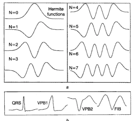
Fig. 1 Hermite functions

a Plots o f the first eight basis functions belonging to the Hermite family of functions;

b Example of a set of ‘shapes’ to be modelled by Hermite functions for a specific application; namely QRSiectopic beat detection

(3)

The second reason for selecting the Hermite function set was motivated by the form of the functions them- selves. Comparing the form of the Hennite functions with typical QRSiectopic beats, i.e. electrocardiogram (ECG) arrhythmia beats (see Figs. l a and b), it seems reasonable to suppose that a series expansion of Her- mite functions may be well suited to provide a concise representation of these signals [2-61. In short, if a signal has a form which shares some resemblance with the form of the basis functions, then its series expansion is likely to have few terms in it, i.e. the ‘spectra’ has a ‘narrowband’ characteristic. This also means the dimensionality of the feature space is minimised.

Note that the method described in this paper has been applied to the problem of detecting and classify- ing QRS and ectopic beats within an ECG trace [2, 31. Consequently, much of its description lies within the context of this application. Although the method outlined is focused on ECG waveform analysis, its suitability can be extended to signals, e.g. u(t), that suffer simple scale and translation distortions as modelled by au(pt - z). This paper concentrates its discussion on the methodology for determining and using Hermite coefficients. The main contribution of the paper is Section 2 where the Hermite basis is introduced and its use detailed: how to estimate the spectral coefficients, the spread factor, and the shift factor; and the effect of signal scaling, translation and dilation on the spectral coefficients. Also suggestions on estimating the number of terms to use in the series expansion are presented in the context of a specific application.

2 Methodology

2.7 Hermite basis set

The nth-order Hermite function is a weighted function of the nth-order Hermite polynomial. The Hermite polynomials are recurrence relations, and so too are their derivatives [l, 71:

dn

H n ( t ) = i - 1 ) ” e x P ( t 2 ) ) ( e x P ( - t 2 ) ) (1)

H n + l ( t ) = 2 t H n ( t ) - 2 n H n - l ( t ) where H o ( t ) = 1

To minimise precision errors caused during the computation of factorials in the Hermite function normalisa- tion constant, this paper uses the normalised form of the Hermite polynomials (signified by the A notation).

Also, a table-lookup approach is used to replace precomputable functions such as dn.

h 1

H o ( t ) = -

Jz/;;

( 3 )

00

/

exp (

-t2)

Iz,

( t ) R

( t )

dt -02

00

-00

Therefore, { hn(t)} represents the orthonormal basis set of Hermite functions as shown in Fig. la. By replacing

346

t with its scaled version ( t - z)/o, a generalised form of the nth-order orthononnal Hermite function, h,,.(t,

z)

is defined, where

o

is the ‘spread’ of the function and

z

is the ‘shift’ of the function.

hn,u(t, 7)

2.2 Evaluating the Hermite coefficients To determine the Hermite coefficients of signal u(t), the following iiitegral is evaluated:

& ( a , 7 ) = u(t)h,,,(t, r)dt (6)

-cc

.I

Substituting

x

= ( t - z ) / ( d 2 ) into eqn. 6 we obtain

00

u n ( o , r ) =

/ v ? % u ( z n h + ~ ) l ? ~ ( z \ / T )

e x p ( - z 2 ) d z

( 7 ) To evaluate this integral, the Gauss-Jacobi integration theorem is used [I, 81

(-m

<

03) ₍₈₎

where the set of weights wi is known.

If p(x) is defined as an exponential weighting function, exp(-x2), then the optimum grid points are the roots of the (A4

+

1)th Hermite function (i.e. the Mth- order Hermite function). If these points are examined, we find that they are unevenly spaced, i.e. the outer- most points are further apart than the points near t = 0. To compute the roots of HM and its corresponding weights, the algorithm by Secrest and Stroud is used [9], p.154.

The first task is to exploit the form of eqn. 8 by rewriting the integrand of eqn. 7 as the product of two functions,

Ax)

and p(x), where

p(x)

is defined as an exponential weighting function:

p ( z ) = e x p ( - z 2 ) (9)

If we assume u(x) is a polynomial such that

fn,o(x,

z)

is also a polynomial of at most degree ( 2 M - l), then the spectral coefficients are

M-1

2=0

If no such assumption is made, then the equality of eqn. 11 becomes an approximation, i.e. the spectral coefficients are estimates.

2.3 Estimating the Hermite spectral coefficients for a discrete time signal

The previous subsection has shown how the spectral coefficients for the Hermite basis set can be determined for continuous-time signals. Since most signals are represented in a time sampled form, it would be useful if

(4)

eqn. 11 could be used accordingly. Unfortunately, there is no integer-based quadrature technique since the manner in which the spectral coefficients are determined makes it necessary to know the value of the signal, i.e. u(x), at the grid points; which have noninteger values and thus lie between the sample points of the signal. To get around this problem, interpolation is done; e.g. zero-order holding or linear interpolation. Experimental results on the signals in Fig. l b have shown improvements in the fit (i.e. squared error) between a signal and its synthesised form when linear interpolation is used instead of zero-order holding. Note that because of interpolation, the equality in eqn. 11 is replaced by approximation.

If the grid values (or roots) of HM are examined, one finds M values

{xo,

xl,

...,

x ~ - ~ } , such that

xo

> x1 >

...

> xM-l. Note that

(i) for M odd;

f,,dO,

Z) = 0 for n odd; xM, = 0 and xMn+l+z =

-x,

where i E {O, 1,

...,

M/2 - l}.

(ii) for M even; = -x, where i E (0, 1, ..., M/2 - 11.

With this in mind, eqn. 11 is rewritten as Ml2-1

U n ( 0 , T ) = W z [ f n , & z , T )

+

f n , 0 ( - % 4 ]

n = 0 , 1 , .

. .

,

N - 1

t=O

(12) However, the following expression is used in the case where M is odd and n even:

an(a, .) = W M / 2 f n , d O , 7 )

M l 2 - 1

+

w z [ f n o ( G , T )

+

f n , o ( - G , 4 1

2=0

(13)

Also from eqn. 10, and given that u(t) is a continuous-time form of a discrete time signal of finite duration, i.e. (2L

+

l ) samples, the range of values for t for which u(t) = 0 is, It1 < L or equivalently

-(z

+

L ) / ( d 2 )

> x >

(L

- z)/(d2); given the substitution used in eqn. 7. Referring to eqns. 12 and 13 we need not evaluate the entire summation over the interval i = 0 to

(Mi2 - 1). Instead the minimum value of

k

is found such that xk 5 (abs(z)

+

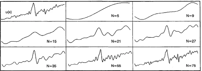
L ) / ( d 2 ) . Then the summation interval of eqns. 12 and 13 becomes i = k to (M/2 - 1). Fig. 2 demonstrates the modelling of a typical discrete- time, finite duration signal for various values of N

where N is the number of Hermite coefficients. It also shows that the Hermite series representation is not par-

N -

N=35

ticularly efficient when modelling a typical discrete- time, finite duration ‘wideband’ signal, i.e. a signal which has both low and high frequency components. However, in the following Section 2.4.4, an approach is considered to selectively model the relevant component within such signals.

//--

N=5

AA

>>

N=55

2.4 Estimating the spread/shift value

In the previous subsection, a procedure for computing the Hermite coefficients was outlined, where the spread and shift term have fixed real values. This Section investigates methods to estimate the spread value, where such methods can be similarly applied to the estimation of the shift value. Since the theory for choosing an optimum spread is still incomplete, LMS techniques are used instead. After each estimate of 0,

the coefficients are recalculated and the iterations con- tinue until a solution is reached. Note that if the spread value is chosen poorly then a large number of series expansion terms are required to produce a satisfactory fit. Also, this relationship between (r and N is a significant one as emphasised in [lo]. In this subsection various optimisation techniques [ 1 11 are considered to estimate the spread for a fixed N . They, however, do not guarantee the spread to be optimal, i.e. finding the global minimum of the cost function.

Consider the discrete-time signal (interpolated) u(t), and its synthesised form, uN,dt). The error-sum (cost) function, EN(c)), is defined as the squared error between these two signals. To minimise this error, two well- known methods, namely the step-search approach and a gradient descent approach have been tried; see the Appendix for details.

2.4.

I

Step-search approach: The step-search approach to selecting

o

that minimises the error sum involves computing the error sum at various values of

o,

within the range

omin

I

o

I

omax,

as

o

moves in constant A o increments; and choosing the value of (r with the least error sum. This method requires that the search range of o be known a priori together with its step size. Although this approach is computationally expensive, especially if the step size is small, the solution it provides is a ‘ball-park’ estimate of the global minima.

2.4.2 Gradient descent approach: This approach is computationally less expensive than the step-search method. Two methods that adopt this approach, i.e. steepest-descent and Newton’s method, are presented below; see the Appendix for equations.

/

N=9

vJ^-J\/Jv’

N=27

M

N=75

i of N orthonortnal

(5)

Steepest descent method. The steepest descent method involves adjusting the value of o after each iteration as given by eqn. 14; see also eqns. 30, 31 and 32 in Section 7.1. See [4, 51 for a similar proposition. After each adjustment of o, the coefficients are recomputed with this new value of CT using the method outlined in earlier

sections:

ok+l = f l k -

XvI,

(14) where

A

2 0 and V k is the error gradient

Newton's method. Newton's method is similar to steepest descent. However, unlike steepest descent, there is no step-size parameter A. Instead, the second derivative is used and the adjustment of o is given by eqn. 15; see also eqns. 33, 34 and 35. This method converges rap- idly but is sensitive to the initial value of o. It works especiaily well for problems where the 'error surface' is quadratic in form.

(15) vk

v k k

f l k + l = f l k - -

where Vkk is the derivative of the error gradient.

2.4.3 Combined approach: Given the strengths and weaknesses of the step-search and gradient descent methods, it seems only appropriate to use both approaches to increase the likelihood of finding an optimum solution for the spread. The combined method would involve the following stages.

Stage 1. Step-search method. Here a sparse step-search is made to minimise the computational expense and provide a 'ball-park' estimate of the global minimum.

Stage 2. Steepest descent method. Since the initial value provided by stage 1 is only an estimate and could well be far from the solution, the steepest descent method is employed to provide a better estimate. It is preferred over Newton's method because it is far better behaved in the presence of a poor initial estimate.

Stage 3. Newton's method. Newton's method is used in the final stage because of its fast convergence. Also, it is assumed that the initial spread value provided by stage 2 is a good enough estimate to guarantee the nonchaotic behaviour of this final stage.

The maximum number of iterations is fixed when implementing such an algorithm in a time constrained application. This is because the maximum computation time allocated for the algorithm to complete its task has to be known a priori to guarantee known behaviour. Therefore, gradient descent algorithms usually have as their stopping criterion the following condi- tions: (i) V k = 0, or (ii) k > MAXITERATIONS; which ever is satisfied first.

2.4.4 Problems with local minima: To illustrate problems inherent in selecting an optimum CT when

using gradient descent techniques, consider the following example. Note that this example seeks to demonstrate how the presence of more than one local minima can cause methods like steepest descent to fail; and how, through 'preprocessing' the signal, the 'landscape' of the cost function can be changed to favour the intended minima.

To begin, a test case is generated, i.e. signal s(x) as defined by eqn. 16, which contains a high-frequency component (spike) and a low-frequency component (linear trend). Next s(x) and w ( x ) are multiplied

348

together to create a signal u(x) = w(x).s(x) that provides more than one dominant local minima, i.e. local minima with comparable error sum values. This is done to provide a scenario that emphasises the difficulties in picking the 'right' minima.

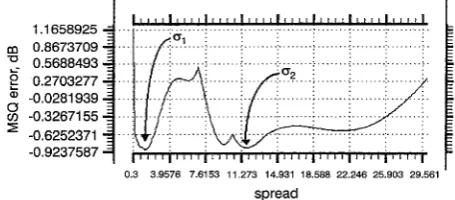
Figs. 3-5 demonstrate that selection of the value of the spread o, at the first 'local minimum' isolates the 'high- frequency' signal in s ( ~ ) , i.e. the spike. Alternatively, by selecting the next spread value, 02, at the next 'local

minimum', a signal of 'lower frequency' i.e. the linear trend component, is isolated. The relation between the spread and frequency is an intuitive one, i.e. the smaller the spread value, the higher the frequency. The spread parameter is also a useful feature for measuring the 'width' of a signal's shape. Note that this particular example typifies the problem of detecting QRS com- plexes in ECG signals with severe baseline wander.

a

...

U

0

...

b

Fig.3

a Typical signal, s(x), with a high-frequency spike and a low-frequency linear trend

b Signal windowed, u ( x ) = s(x) w(x), to provide comparable local minima Example of more than one 'optimum'

I .I 658925 m 0.8673709

T-

0.5688493

g 0.2703277

'

-0.0281939

%

-0.3267155 -0.6252371 -0.9237587

I

0 3 39576 76153 11 273 14931 18588 22246 25903 29561

spread

Fig.4 Error sum for various values of B for the signal from Fig 3b

(6)

a

I I

b

Fia.

-

5 Simal reconstructions i N = 51 based on Fic. 4

a High-freqiency spike, ~~,~,(x), 'reconstiucted by sele&ng the lower of the two minima, 0,

b Low-frequency signal, pN,02(x), reconstructed by selecting the higher of the two minima, 0,

Returning to the problem of detecting a beat in an ECG, consider the scenario where the ECG waveform is processed as a series of running snapshots of partial ECG waveforms as viewed through a sliding window that traverses the full ECG waveform in time. Clearly only when the beat to be recognised occupies a central position in the window, is the beat considered detected. This means that the signal information at the centre of the window is more relevant than that at the ends. In other words the fit of the signal segment located in the central portion of the window should be better than the segments at the ends. To reflect this in the overall fit, the error contributed by the samples at the end of the window have less weight than those in the middle; hence the error term is redefined as

biased error sum,

(18) where m is equal to the sample width of the signals, i.e.

= 0.6L.

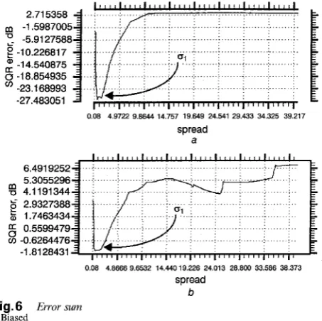
From Fig. 6a note that the biased error sum alters the cost function 'landscape' such that only a single minima is left, thus making the selection of an optimum spread simpler.

The previous attempt to remove the undesirable local minima works only for signals whose relevant information all lie within the regions of the window of similar size. Therefore

if

there are signals with vastly different widths (i.e. frequencies), erroneous local minima are usually the minima with the largest spread values and can be attributed to some linear trend component within the signal. As an alternative to using a biased IEE Proc -Vis Image Signal Process, Vol 144, No 6 December 1997

error sum, the unbiased error sum is used. It is defined in terms of u(x) whose linear trend component has been removed. To carry out this removal, a straight line is fitted through u(x) using linear regression, and then u(x) is redefined by removing this linear component within it. Fig. 6b shows that the error sum after removal of the linear trend effectively creates a single minima, thus making the selection of an optimum spread simpler.

, ~ ~ ~ I ~ ~ ~ ~ i ~ ~, I # , , , I ~ ~ I ~ ~ ~ ~ I ~ I , ~ I , , , , I , ~ ,

e

-10226617

2

-14 540875

8

-1 8 854935 -23 168993

-27 483051

008 49722 98644 14757 19649 24541 29433 34325 39217

spread a

I , I I I I , , I c l , , , , I , , , 0 1 1 I , , I , , , I I , I , , I , , I , I ,

6 491 9252 5 3055296

% 41191344 2.9327388

5 1.7463434

-1 8128431

I " " I " " I " " I " " I " " 1 " " 1 ~ " ' I '

0 0 8 4866696532 1444019226 24013 28800 33586 38373 spread

b

Fia.6 Error sum

a E h e d

b Unbiased, but with linear trend removed from u(x)

N = 5 in all cases

2.5 Overview of results

To determine a suitable combined estimation approach, experiments were carried out using five test signals. These were signals QRS, FIB, VPBl and VPB2 of Fig. lb, and a signal with arbitrarily chosen Hermite parameters as shown in Fig. 7a. They were represented as sampled signals of 200 samples each (i.e. -100 5 t 5 100) and taken from the synthesised form of the signal as defined by their Hermite parameters.

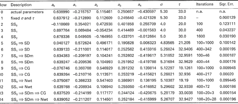
Using the estimation techniques outlined earlier, various permutations of the combined approach were tried; see the second column of Table 1. In the first stage of this approach, a step-search is adopted to estimate a starting point for use by the subsequent gradient descent stage. This is done by imposing a uniform grid of CY and z values across a fixed range of values

and computing the error sum at every point in the grid. Then the (0, z) pair with the smallest error sum is cho-

sen. Note that for certain applications, this grid need not be uniform, but random or user defined to minimise the number of grid points searched. Also, the Her- mite coefficients are recalculated for every point in the grid and after every adjustment to 0 and

z

during the

gradient descent optimisation process. Therefore, if a signal s(t) has an error-sum minimum that lies at (0, 0),

then the error-sum minimum of the signal s(t -

z)

will lie at (0,

z),

see Figs. 7a and b.

(7)

Table 1: Results of various optimisation procedures for estimating the Hermite coefficients, o a n d z of a signal (200 samples) as defined by the first row‘s parameters

0 1 2 3 4 5 6 7 8 9 10 11 12 13 14

Row Description a, a, a2 a3 a4 cf z Iterations Sqr. Err.

actual parameters 0.638990 -0.215757 0.1 15461 0.250657 -0.430597 5.30 33.0 n.a. n.a.

fixed o a n d z 0.637912 -0.212890 0.112609

sso -0,118669 0.354021 0.472938

SSl 0.697764 0.069484 -0.054234

ss2

0.678336 0.049505 -0.164955

SS, =$ SD 0.040127 0.572624 0.496171

SS, 3 SD 0.639133 -0.211001 0.114017

SS, 3 SDm 0.634383 -0.209197 0.104241 SS, 3 SDm 0.639247 -0.209536 0.104993

SS,

+

CG -0.076746 0.360708 0.546929

SS,

+

CG 0.639264 -0.210716 0.113571

SS,

+

N w t -0.075087 0.366233 0.547403

SS,

+

N w t 0.639768 -0.208934 0.106940

SS, j SDm 3 CG 0.637520 -0.214199 0.117177

SS, 3 SDm

+

N w t 0.639052 -0.211207 0.114501

0.245640

0.401858

0.414469

0.43370 1

0.190828 0.252562 0.252602 0.251952 0.391232 0.253219 0.386901 0.255050 0.2441 24 0.252184 -0.421328 0.255709 -0.001563 -0.012664 0.008323

0.41 591 6

-0.419617 -0.419788 0.139814 -0.415621 0.136195 -0.416852 -0.420675 -0.415999 5.30 4.0 4.0 5.0 4.83565 5.26824 5.31852 5.31694 5.12297 5.26821 5.10387 5.29602 5.28179 5.26707

33.0 - 0.000 129

20.0 100 0.1231 11

30.0 400 0.043237

30.0 1600 0.030190

21.205 100+1000 0.100142

32.9406 400+342 0.000195

32.9591 100+46 0.000187

32.9629 400+44 0.000176

19.1261 100+1000 0.009945

32.936 400+217 0.00020

19.19 100+1000 0.099445

32.9338 400+72 0.000186

33.0038 100+20+3 0.000154

32.9427 100+20+28 0.000196 ~

Procedures

SS,= Step-search across a 10 x 10 uniform grid; SS, = Step-search across a 20 x 20 uniform grid; SS, = Step-search across a 40 x 40 uniform grid; SD = Steepest descent; Lo = 1.0; L, = 10.0; SDm = Steepest descent w/momentum; ;1, = 1.0;

CG = Conjugate gradient; La = 1.0; N w t = Newton‘s method.

Stopping criterion

(1) Sqr. Err. < 0.0002; or (2) Number of iterations (by stages > 1) 2 1000

= 10.0; pa = 0.5; & = 1.0.

= 10.0.

12, 9 ) for VPBl and (11, 14, 7, 12, 10, 5, 8, 9, 13, 6 )

for VPB2. Therefore, given the desired approach must take as few iterations as possible and must always reach the solution, the approach SSo

+

SDm +Nwt (row 14) was selected and used by the applications described in [2, 31.

a

b Fig. 7

a s(t ~ z)

b Error sum surface of ~ ( t ~ z)

Error-sum surface for a ‘shifted’ signal with respect to o and z

2.6 Effect of signal scaling, translation and dilation on He rm ite coefficients

In this Section the effects of signal scaling, translation and dilation on its Hermite spectral coefficients, spread term and shift term are determined. The influence of these three common transformations is particularly important because they are a first-order approximation

350

of the kinds of typical distortions experienced by signals. Consider a signal u(t) whose Hermite spectral coefficients are {bo, bl,

... .

bNpl} for some spread

o,

and shift z,, which have been determined such that the squared error of the fit is minimised, i.e.

N-I

i=O

Let signal v(t) be defined as a scaled version of signal

u(t), with Hermite spectral coefficients {CO, cl,

...,

c ~ - ~ }

and spread 0, and shift z, or equivalently described

with Hermite spectral coefficients {ao, a l ,

...,

u ~ - ~ } and spread

ovv.

v ( t )

= olu(Pt - T ) where a ,

p

and ‘r are scalars

(20)

u ( t ) = UN,,,

( t )

N-1

i=O N--1

i=O

The parameters

z,,

0, and

e,

can

be rewritten

in

terms of

z,,

o, and b, as follows,

w h e r e p > o a n d n E { O , l ,

. . . ,

N - l } (22) Also, if z = 0 in eqn. 20 then,

(8)

In summary, the relationships of eqns. 22 and 23 provide a means for estimating the Hermite coefficients, spread and shift for a distorted signal, v(t), using the known parameters of the undistorted signal, u(t), and the distortion, as given by parameters

z,

p

and

a.

In addition, by comparing the Hermite model parameter estimates of u(t) with that of v(t), the values of the distortion parameters can be determined.

The results of eqns. 22 and 23 are particularly useful because they provide a method for describing a signal by appropriately defining the feature vector in terms of the signal's Hermite model parameters. For example, if there is to be no discrimination between a signal u(t) and its distortion au(Pt), then the norm of its Hermite coefficients is taken:

= r ( a u ( P t ) ) (24)

where T(u(t)) defines the feature vector of signal u(t)

and represents a feature extraction process on u(t).

Similarly, if there is a need to discriminate between a signal's scale distortions in time but not in magnitude then,

q u ( t ) )

=

[a,

iqT

=

r(aU(t))

#

r(.U(pt))

where

/3

#

1 ( 2 5 )

Hence by choosing the features in the manner similar to that described by examples eqns. 24 and 25, the type of discrimination between signals can be predefined.

2.7

Order

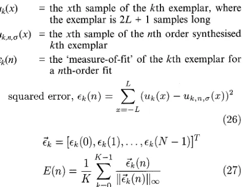
estimation

Evaluating the order of our series expansion is very much dependent on the 'patterns' to be classified. Since these patterns are known (and it is assumed that there are K exemplars of their typical form), a value for the order, N , is chosen such that there is no significant improvement in the fit for the order greater than N . To do this, some measure of the fit is required. Two such 'measures' are considered i.e. the squared error and the correlation coefficient.

Considering the squared error as the first measure of the fit.

uk(x) = the xth sample of the kth exemplar, where

U ~ , ~ , ~ ( X ) = the xth sample of the nth order synthesised

~ ~ ( n ) = the 'measure-of-fit' of the kth exemplar for the exemplar is 2L

+

1 samples long

kth exemplar

a nth-order fit L

squared error, e k ( n ) = (uk(z) - U ~ , ~ , ~ ( Z ) ) ~ x=-L

(26)

K-1 \

The maximum value for the normalised averaged error, E(n) is unity for n E (0, 1,

...,

N - l}. In general, n = 0 has the worst fit, which implies E(0) = 1. Let the order be n when E(n

+

1) 2 E(n). This condition for picking n does not always work and depends on the convergent properties of the exemplars i.e. the inequality is satisfied for large values of n only.

IEE Proc.-Vis. Image Signal Process., Vol. 144, No. 6, December 1997

Next consider the correlation coefficient as the measure-of-fit [13] i.e.

suv

linear correlation coefficient, &k ( n ) =

su(k)su(k)

where U =

u ~ ( x )

and U = u ~ , ~ , ~ ( x ) ₍₂₈₎ As long as it is of no consequence that the synthesised signal is a linear function of the original signal (i.e. it could be scaled and/or have its mean shifted), it is safe to interpret eqn. 28 as a measure of fit to use.

When the average correlation coefficient E(n) equals unity, there is a perfect fit. Similar to the least squares approach, n is chosen such that E(n

+

1) I E(n). Once again, depending on the convergent properties of the exemplars, this inequality may only be satisfied for large n. Although the basis functions satisfy completeness, there will be a point beyond which there will be no 'significant' improvement in the fit. At this point the truncation error is small and susceptible to precision errors. These errors give rise to an overall error sum that oscillates along a decreasing long-term trend (see Fig. 8). Since this tends to occur for large n, the inequality is modified such that the order is chosen as the smallest value of n that satisfies, E(n) 2 E , for a predetermined threshold E,.

-"''2'-

C 0.7131924

-6.5168552 -7.206862

1 5 9 13 18 22 26 30

order n a 1.0026458

0.94516434

1

7

k0.2549848

0.298583

I ' ' ' ' I ' ' ' ' I ' ' ' ' I ' I ' ' I ' ' ' I ' ' ' ' I ' ' ' '

' '

!% 0.8876828i 0.8302012

[

0.21 13867 0.16778855

0.1 241 9042 0.0805923 = 0.0369941

f

-0.006604

2 0.7727197 0.7152382 0.6577566 0.6002751

1 5 9 13 18 22 26 30

order n

b Fig.8

a E(n) defined as sum of squared errors, E ( l ) = 0.24 b E(n) defined as correlation coefficient, E(l) = 0.60

Plots of E(n) and dE(n)/dn versus N for various definitions of

E(n)

This inequality does not particularly suit the least squares approach because ETH is arbitrarily chosen. The correlation coefficient, however, lends itself to the 'threshold' inequality because it is a measure that is not influenced by the scalar variations of u(t), and it is intuitively more meaningful.

To estimate a suitable n, we can either be conservative or liberal in our choice. We define a liberal selection by picking n for which the correlation coefficient 2

0.95 and conservative, by picking n for which the correlation coefficient 2 0.99. From Fig. 8, these values of n

are 5 and 11 for the liberal and conservative approach, respectively.

3 Applications

The representation of a 1-D signal as a series expansion of Hermite basis functions and the subsequent use of the coefficients of this series expansion as features towards signal analysis has been successfully applied to the area of ECG waveform analysis. The suitability of

(9)

Hermite coefficients as morphological features in QRS detection was first suggested by Sornmo et al. [6]. However, no method for estimating these coefficients was proposed. Since then, Laguna et al. [4, 51 have also investigated the use of Hermite coefficients together with an associated spread term for QRS and ectopic beat detection. However, they did suggest a method for estimating the Hermite coefficients. Theirs was a scheme based on the adaptive linear combiner [13], called the adaptive Hermite model estimation system (AHMES). It used LMS estimation to estimate both the coefficients and the spread term. While the AHMES approach is well suited to tracking an ECG signal, it is unclear if the coefficients and spread term model the ‘shape’ of the beats and if they can indeed be interpreted as shape features.

Unlike the AHMES system, where the approach seeks to minimise the squared error of each ‘incoming’ sample, the authors have proposed an approach in [2, 31 which seeks to minimise the squared error of each ‘incoming’ signal segment. In other words, the cost function is the sum of the squared errors of all the samples taken over a user-defined period within which the shape of signal to be modelled lies. Note that the length of this user-defined period is a heuristic choice such that the ‘shapes’ being looked for in a signal all fit within this period. Hence the length of this period is determined by the shape with the largest ‘width’.

It is worth noting that the first Hermite basis function has the form of a Gaussian distribution and all subsequent Hermite basis functions are derivatives of this form. This could suggest that the Hermite series expansion may be well suited to modelling ‘distribu- tions’.

4 Conclusions

The selection of an appropriate orthogonal basis function is very much dependent on the shape of the signals to be modelled. This choice involves fmding an orthogonal set of basis functions which most conservatively models the types of ‘shapes’ intended for recognition. More often than not, the close morphological similarity of these functions to the ‘shapes’ provides a good indi- cation of their suitability.

In this regard, this paper has purposely considered the orthonormal Hermite basis set given, the suitability of the Hermite parameters in modelling the one-dimensional shapes found in signals such as ECG traces. This paper has outlined a methodology to estimate the Her- mite-spectral coefficients of a one-dimensional signal and its associated spread andlor shift term values.

It is worth noting that the deterministic approach to estimating the Hermite spectral coefficients of a I-D signal, as described in this paper, allows the method to constrain the use of LMS estimation techniques to just the two (one) variables, i.e. the spread and (or) shift term. As a consequence, the visualisation of the search space ‘landscape’ for these two terms is now a practical proposition. From such visualisation, the problems in trying to estimate an optimum spread and shift term value, like false minima and nonconvergence were addressed. In addition, heuristic approaches to estimating the number of coefficients to use were suggested, and special attention was given to determining the influence of common signal distortions such as scalar, dilatory and translatory effects, on the Hermite coefficients, spread and shift parameters.

352

5 Acknowledgments

We wish to thank the PhD and Scholarship Committee of the University of Western Australia for supporting this work through the University Research Scholarship Award. , 6 1 2 3 4 5 6 7 8 9 References

ABRAMOWITZ, M., and STEGUN, L.A.: ‘Handbook of mathematical functions’ (Applied Mathematics Series, vol. 55, Dover Publications, 1968)

RASIAH, A.I., and ATTIKIOUZEL, Y.: ‘Syntactic recognition of common cardiac arrhythmias’. IEEE Eng., Biology and Medi- cine Society 16th annual international conference, November 1994, Baltimore, USA

RASIAH, A.I., and ATTIKIOUZEL, Y.: ‘A syntactic approach to the recognition of common cardiac arrhythmias within a single ambulatory ECG trace’, Australian Computer J., 1994, 26, (3), pp.

102-112

LAGUNA, P., CAMINAL, P., THAKOR, N.V., and JANE, R.: ‘Adaptive QRS shape estimation using Hermite model’. 1 lth IEEE annual conference of Eng., Medicine and Biology Society, 1989, pp. 683-684

LAGUNA, P., JANE, R., and CAMINAL, P.: ‘Adaptive feature extraction for QRS classification and ectopic beat detection’, Pro- ceedings Computers in Cardiology, 1992, IEEE Computer Society Press, pp. 613-616

SORNMO, L., BORJESSON, P.O., NYGARDS, M., and PAHLM, 0.: ‘A method for evaluation of QRS shape features using a mathematical model for the ECG’, IEEE Trans., 1981,

BMlG-28, (lo), pp. 713-717

GRADSHTEYN, IS., and RYZHIK, I.M. ‘Table of integrals, series and products’ (Academic Press, 1980), pp. 1033, corrected and enlarged edition

BOYD, J.P.: ‘Chebyshev and Fourier spectral methods’ in BREB- BIA, C.A., and ORSZAG, S.A. (Eds.): ‘Lecture Notes in Engi- neering 49’ (Springer-Verlag, 1989)

PRESS, W.H., VETTERLING, W.T., TEUKOLSKY, S.A., and FLANNERY, B.P.: ‘Numerical recipes in C. The art of scientific computing’ (Cambridge University Press, 1992), Chap. 4, pp. 147-161, 2nd edn

10 BOYD, J.P.: ‘The asymptotic coefficients of Hermite functions’, J. Computat. Phys., 1984, 54, pp. 382410

11 FLETCHER, R.: ‘Practical methods of optimization’ (Wiley, 1987). 2nd edn

12 SPIEGEL, M.R.: ‘Probability and statistics’ (Schaum’s Outline Series, McGraw-Hill, 1988

13 WIDROW, B., GLOVER, J.R., MCCOOL, J.M., KAUNITZ, J., WILLIAMS, C.S., HEARN, R.H., ZEDLER, J.R., DONG, E., and GOODLIN, R.C.: ‘Adaptive noise cancelling: principles and applications’, IEEE Proc., 1975, 63, (12), pp. 1692-1716

7 Appendix

7.

I

Estimating the spread value

u(x) = discrete time, finite duration signal for x E

U ~ , ~ ( X ) = synthesised signal from N Hermite coefficients with a spread of 0

~ ~ ( 0 , x) = the error between u(x) and U ~ , ~ ( X ) at the kth iteration

{-L, ...) L }

error sum,

L L

x=-L x = - L

(29)

n = O

(10)

-(an

+

1)&

(y)

x

+

_4)(n

+

_{3 ) ( n}

+

_2)(n

+

1)&+4

( Z )

- J ( n

+

2)(n

+

l)kn+z

(E)

-(n2+n+l)&

(31

(35)

1

2

+ - J n ( n - 1)(n - 2)(n - 3)fin-4

7.2 Estimating the shift value

As demonstrated in Section 2.6, the Hermite coefficients are translation variant, i.e. the Hermite coefficients for a signal u(t - z) differ for different values of

z. When a shift term, T, is introduced into the defini-

tion of the Hermite basis function, as given by eqn. 5 ,

then least-squares estimation can be used to estimate a value for z; such that the Hermite functions of eqn. 4 are fitted about t =

z.

In the previous Section, the equations for estimating a spread value for a fixed shift value (i.e.

x

= t -

z)

were presented. Now the remaining cases are considered: (i) estimating the shift value for a fixed spread value; and (ii) estimating the spread and shift value. Note that after each adjustment in value to the spread and/or shift parameter, the Hermite coefficients are recomputed.

7.2.1 For constant

s:

Using eqns. 36 to 39, the same LMS techniques are used to estimate the shift value.

x

[

J ( n

+

1)(n

+

2)I;Tn+2

(q)

IEE Proc.-Vis. h u g e Signal Process.. Vol. 144, No. 6, December 1997

x=-L

7.2.2 For variable 0: Once again, the techniques of the previous Section are employed with some notable changes and additions. First, the second derivative of the error sum function is now defined by eqn. 44 and its inverse, i.e. the Hessian matrix, is required for New- ton's approach. Next, two more gradient descent techniques are introduced: (i) steepest descent with a momentum term; and (ii) conjugate gradient.

- ( n

+

2 ) J n + l H n + 1

(5)

+ J n ( n - l ) ( n - 2 ) & 4

(31

- ₍₄₁₎

The motivation for steepest descent with momentum comes from having found that a typical error-sum surface has significant portions that are 'flat'. Therefore the introduction of a momentum term may prove use-

(11)

ful in reducing the convergence time. We have also found it useful to include eqn. 47 which drops the momentum to zero when an ‘overshoot’ (as given by the predetermined AETHRESHOLD) occurs (see Fig. 7b).

With conjugate gradient, if the error-sum surface is of ‘quadratic’ form, then a faster convergence can be expected:

(48)

vk+l vi,