A b s t r a c t. In the present study, the application of a back propagation) neural network for the prediction of moisture content of barberry fruit (berberis vulgaris) during drying was investiga-ted. The important parameters, namely, pretreatment (no pretreat-ment, heat shocking, olive oil + K2CO3), air drying temperature (60, 70 and 80°C), air drying velocity (0.3, 0.5 and 1 m s-1) and time (s) were considered as the input parameters, and moisture content as the output of the artificial neural network. Experimental data obtained from a thin-layer drying process were used for training and testing the network. Several criteria such as training algorithm, learning rate, momentum coefficient, number of hidden layers, number of neurons in each hidden layer, and activation function were given to improve the performance of the artificial neural net-work. The best training algorithm was Levenberg-Marquard with the least mean square error value. Optimum values of learning rate and momentum for the artificial neural network with gradient descent momentum training algorithm were set at 0.5 and 0.7, respectively. The optimal topologies were 4-20-1 and 4-25-5-1 with mean square error values of 0.00318 and 0.001 with logsig activation functions. Also, with tansig activation function, the optimal topo-logies were 4-20-1 and 4-15-15-1 with the mean square error values of 0.00293 and 0.00130. There was no significant difference between the two activation functions in optimal topologies. There was good correlation between the predicted and experimental values in optimal models.
K e y w o r d s: thin-layer, artificial neural network, moisture content, training algorithm
INTRODUCTION
Barberry fruit (Berberis vulgaris) is known as a medici-nal and ornamental plant in the world (Aghbashloet al., 2008). Medicinal use of barberry dates back more than 2 500 years, and it has been used in Indian folk medicine to treat diarrhoea, reduce fever, improve appetite, relieve upset
sto-mach, and promote vigour as well as sense of well-being. Iran is the largest producer of barberry in the world (Fathol-lahzadehet al.,2008). Dehydration of agricultural products in the tray dryer involves a high energy consumption mainly because the operation control and maintenance are made heuristically. Too high moisture content leads to microorga-nism growth and low quality, while too low moisture content may lead to excessive energy consumption (Lertworasirikul and Tipsuwan, 2008). To achieve an increase in the process efficiency and to reduce the energy consumption, the pro-cess parameters have to be optimized (Aghbashloet al., 2009; Akpinaret al., 2003; Aviaraet al., 2010). A convenient way of getting to this target is to numerically simulate the total system behaviour and to predict the main parameter evo-lution for different operational conditions (Margaris and Ghiaus, 2006). The main obstacle for extensive analysis of the dehydration process by numerical simulation is the lack of knowledge on the thermophysical properties of most of the agricultural products. On the other hand, the results from numerical simulation have to be validated by means of experimental investigation. Mathematical correlations usually give the most accurate results only in specific experiments and they are not valid in other conditions (Movagharnejadet al., 2007). Besides, mathematical models simulate the drying process based on some assumptions while neglecting the effect of some interdependent variables, which results in de-creased prediction capability (Tripathy and Kumar, 2009). Neural networks have many attractive properties for the mo-delling of complex process. Several studies demonstrated the significance and usefulness of the artificial neural net-work (ANN) in modelling the drying process (Behroozi
Designing and optimizing a back propagation neural network to model
a thin-layer drying process
S. Gorjian*, T. Tavakkoli Hashjin, and M.H. Khoshtaghaza
Department of Agricultural Machinery Mechanics, College of Agricultural Engineering, Tarbiat Modares University, Tehran, Iran
Received March 4, 2010; accepted November 23, 2010
© 2011 Institute of Agrophysics, Polish Academy of Sciences
*Corresponding author’s e-mail: [email protected]
A A
Agggrrroooppphhyhyysssiiicccsss
Khazaee, 2003; Farkaset al., 2000a, 2000b; Sablani and Rahman, 2003; Satish and Pedy Setty, 2005), food temperature prediction during solar drying (Tripathy and Kumar, 2009), predicting moisture content of agricul- tural products (Topuz, 2009), moisture content and water ac-tivity prediction of semi-finished cassava crackers (Lertwo-rasirikul and Tipsuwan, 2008), moisture content modelling of thin-layer corn during the drying process (Trelaet al., 1997), prediction of physical property changes of carrot during drying (Kerdpiboonet al., 2006). Also, a neural net-work has been used to model an industrial drying process and thin-layer drying kinetics (Assidjoet al., 2008; Khazaei and Daneshmandi, 2007) and for the modelling of tomato drying (Movagharnejadet al., 2007).
The aim of this study was to verify that an ANN model can be used to predict the moisture content of barberry fruit during the drying process under different drying conditions. In addition, a method to obtain representative learning data and several criteria to provide an optimal training of the ANN are proposed. The paper is organized as follows: 1. the experimental procedures are described,
2. the ANN was first trained using a database of data sets obtained experimentally,
3. was the optimization of parameters, establishing some criteria to optimize the training process and the learning database were nade (the optimization was made by con-sidering the type of the learning algorithm, different va-lues of momentum coefficient and learning rate, the number of hidden layers and the number of neurons in each of them, and the type of activation functions), 4. the accuracy of the various proposed prediction models
was tested trough the comparison of predicted values with experimental data using linear regression analysis.
MATERIALS AND METHODS
The moisture content of fresh berries was determined by drying in an oven at 105°C for 4 h until the mass did not change between two weighing intervals, performed in tripli-cate (Aghbashloet al.,2008). Chemicals used for dipping the samples were of technical grade. To expedite drying by breaking the waxy layer of barberry skin, thermal shocking of the berries was carried out by immersing them in hot water, followed by cooling with cold water. To increase the water permeability of the skin, the berries were also dipped in a suspension of commercial olive oil and K2CO3. The so-lution of the desired concentration of K2CO3was prepared in distilled water and heated to 50°C, on a hot plate with magnetic stirring. Olive oil was then added to this solution which was kept under continuous agitation during dipping of berries. The test treatments were as follows:
– no pretreatment;
– E1: dipped in hot-water at 85°C for 60 s followed by rinsing with cold water at 10°C immediately;
– E2: dipped in emulsion of 3% olive oil and 6% K2CO3at
50°C for 2 min.
The drying experiments were performed using a labora-tory-scale cross-flow hot-air dryer available at the Agricul-tural Engineering Department of Tarbiat Modares Univer-sity, Tehran, Iran. The dryer consisted of a tray, an air flow system, an air drying heating section and the main drying chamber. The dryer was equipped with an automatic tem-perature controller (± 0.1°C), an online weight data recorder using precision balance (0.01 g, A&D Model-Japan), a load cell and an online data logger employing a computer pro-gram that recorded the weight loss of berries at 2 min inter-vals. The experiments were carried out at hot air temperatu-res of 60, 70 and 80°C. At each drying temperature three velocity values were tested: 0.3, 0.5 and 1 m s-1. For quantitati-ve evaluation of the pretreatment effect, an experiment with untreated barberries was also included. To achieve a steady-state thermal condition, the dryer was set to work for about half an hour prior to the experiments. In each drying experi-ment, about 10 g barberries were placed on the tray of the drying chamber in a thin-layer formation. To ensure storage stability, the barberries were dried to a final moisture content below 18 % (w/w). The experiments were repeated three times and the average of the moisture ratio at each time point was used for drawing the drying curves. The moisture ratio (MR) was calculated using the following equation:
MR M M
M M
e
o e
=
-- (1)
where:Mo,M,andMeare initial moisture, moisture at time
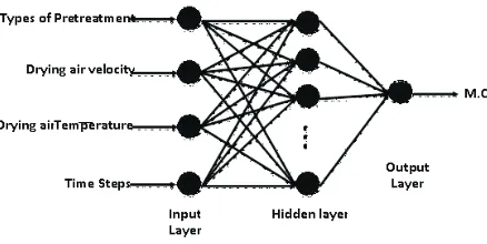
barberry fruits. Each input unit of input layer receives input signalXiand broadcasts this signal to all units in the hidden
layer. Each hidden unitYjsums its weighted input signal and
applies its activation function to compute an output signal as identified in the following function:
Yj fact W Xij i bj
i
= æå +
è ç ç ö ø ÷ ÷ =1 , (2)
where:Wijis the weight of the connection from theith input
to thejth hidden unit,bjis the weight of bias connection for jth hidden unit. The output signal of the hidden unitYjis sent to all units in the output layer. Each output unitOksums its
weighted input signal and applies its activation function to compute its output signal as identified in Eq. (3):
Ok fact V Yjk j bk
j
= æå +
è ç ç ö ø ÷ ÷ =1 , (3)
where: Vjk is the weight of the connection from the jth
hidden unit to thekth output unit. The parameter of bias (b) in Eqs (2) and (3), also called the threshold value, is per-manently set to 1 in the hidden layer as well as in the output layer, so that corresponding weight shifts the activation function along thexaxis. The activation functions used in this study were tangent sigmoid and logistic sigmoid that are defined respectively as (Demuth and Beale, 2003):
f x
x
act( )
exp( )
= +
1
1 , (4)
f x
x
act( )
( exp ( ))
=
+ -
-2
1 2 1. (5)
These two activation functions were utilized in the hidden layers and the linear activation function was prac-ticed the in output layer. The BP training algorithm is an iterative gradient descent algorithm, designed to minimize
the mean of square error (MSE) and mean absolute error (MAE) which are averaged over all patterns and are cal-culated as follows:
(
)
MSE= -å å = = S T n n ip ip i N p M p 2 1 1 0 , (6)MAE= å
-=
1
1
ni Sip Tip
N
, (7)
where:Sipis the desired or actual output,Tipis the predicted
output for the pattern,n0is the number of neurons in the output layer, andnpis the number of patterns.
During training, an ANN is the presented with the data for thousands of times, which is referred to as epochs. After each epoch the error between the ANN output and the desired values is propagated backward to adjust the weight in a man-ner mathematically guarantied to converge. Adjustment of the weightsÄWijcan be calculated as (Topuz, 2009):
(
)
DWij E D
Wij Wij s
=-a ¶ +
-¶ b 1 , (8)
where:ais the learning rate,bis the momentum coefficient and s is the current step. Training is the act of continuously adjusting the connection weights until they reach unique values that allow the network to produce outputs that are close enough to actual desired outputs. The accuracy of the de-veloped model, therefore, depends on these weights. Once optimum weights are reached, the weights and biased values encode the network state of knowledge (Topuz, 2009).
Using experimental data obtained in the thin-layer dryer, an optimized ANN model was developed to predict the outlet moisture content of the barberry fruit. The basic back propa-gation algorithm adjusts the weights in the steepest descent direction (negative of the gradient) (Dayhoff, 1990).
One of the most important tasks in ANN model develop-ment is to find the optimal network architecture. This net-work architecture is to be selected out of several netnet-work con-figurations. Comprising the combination of various model parameters, namely, the value of momentum coefficient and learning rate, the number of hidden layers, the number of neurons in hidden layers, different activation functions and the training algorithm. A list of different training algorithms is summarised in Table 1.
RESULTS AND DISCUSSION
Initially the performance of the ANN was assessed with different training algorithms. In order to obtain the best results, each of the model parameters was varied, keeping the other parameters constant to study the influence of variable parameters. The ANN with randomly chosen tansig activation function, one hidden layer and 20 neurons in the hidden layer, was trained and the best training algorithm that Fig. 1. Scheme of the ANN used for predicting the moisture
can make the ANN model most effective in the simulation of experimental data was selected. The results of the error ana-lysis showing the influence of different training algorithms on prediction of the moisture content are presented in Fig. 2. Among the different training algorithms the LM provided the best results. CGF and OSS were also satisfactory.
In order to acquire the optimum performance of a neural network, the rate of error convergence was checked by ad-justing the learning rate and momentum coefficient. The learning rate and momentum coefficient values affect the ANN performance significantly (Khazaei and Danesh-mandi, 2007). The number of neurons in the hidden layer was 20. In this optimization, GDM algorithm was exploited, that is due toaandbin this algorithm are constant during
training. On the other hand, these parameters in this training algorithm are time independent. In order to illustrate how the ANN was optimized, some of the results obtained during training are given in Table 2. The greater the learning rate, the more the weight values were changed. Too low a ing rate made the network learn very slowly. Too high a learn-ing rate made the weights and objective function diverge. From these results, the learning rate of 0.5 led to the best convergence and the lowest model error. Similar results were reached with the momentum coefficient of 0.7. As can be shown, a small learning rate and large momentum were desirable. Momentum allows a network to respond not only to the local gradient, but also to recent trends in the error surface. Totally, the optimal values of these parameters should be reached by a trial and error method. The networks were trained up to epochs where the level of error was
Learning rate a
Momentum coefficient
b
MAE
0.2 0.4 0.276
0.2 0.4 0.215
0.2 0.4 0.541
0.5 0.7 0.394
0.5 0.7 0.257
0.5 0.7 0.682
0.8 0.5 0.457
0.8 0.5 0.282
0.8 0.5 0.597
T a b l e 2. Results of the ANN training with GDM training algorithm and different values ofaandb
Fig. 2.Results of the ANN model considering different training algorithms.
MSE
Acronym Algorithm GD Gradient Descent
GDM Gradient Descent Momentum
GDX Variable Learning Rate Backpropagation GDA Variable Learning Rate Backpropagation LM Levenberg- Marquardt
RP Resilient Backpropagation CGF Conjugate Gradient BFG BFGS Quasi- Newton OSS One- Step Secant
CGB Conjugate Gradient with Powell/Beale Restarts SCG Scaled Conjugate Gradient
CGP Polak-Ribiére Conjugate Gradient
satisfactory and further cycles had no significant effect on its reduction. In order to obtain the optimum number of hidden layers and the number of neurons in each of them, at first the ANN model was trained with one hidden layer and varying number of neurons in this layer with logsig activation function and LM training algorithm. Then the ANN was trained with two hidden layers and different number of neurons in each layer with the same training algorithm and activation function. The minimum and maximum number of neurons in hidden layers was 5 and 20, respectively, starting with 5 neurons and then increasing the network size by adding 5 neurons each time. The best topologies were 4-20-1
and 4-25-5-1 with MSE values of 0.00318 and 0.001, respectively. The results are shown in Table 3. In the ANN architecture with one hidden layer, the error with 5 neurons was high; by increasing the number of the neurons this error reduced, but when the number of neurons was 25 the error increased again. Using too few neurons in the hidden layers will result in something called under-fitting. Under-fitting occurs when there are too few neurons in the hidden layers to adequately detect the signals in a complicated data set. Too many neurons in the hidden layers may result in over-fitting. Over-fitting occurs when the neural network has so much information processing capacity that the limited amount of information contained in the training set is not enough to train all of the neurons in the hidden layers. When the network begins to over-fit the data, the error in validation set will typically begin to increase (Assidjoet al., 2008). The ANN with two hidden layers was trained and the error was reduced in respect of one hidden layer architecture. These networks, named shallow networks (Amiri Chayjan, 2006), had better performance. Obviously, some compromise must be reached between too many and too few neurons in the hidden layers. In order to assess the performance of the network with two different activation functions, the pre-vious experiments were done with tansig activation function again and the results were comprised (Fig. 3). The best topo-logies with this activation function were 4-20-1 and 4-15-15-1 with the MSE values of 0.00293 and 0.00130, respec-tively (Table 3). Comparison between the two activation functions indicates that except the topologies of 4-5-1, 4-5-15-1, 4-5-5-1 and 4-10-15-1, in other topologies the influence of the transfer functions on the capability of the ANN model made no significant difference. Finally, the pre-diction capability of proposed models was further assessed on the basis of regression line characterized by its correla-tion coefficients (R), between predicted and experimental values for test and validation data sets. The results are presented in Table 4. As can be seen, the results predicted by those topologies that have the least error were found to be slightly closer to experimental data.
Number hidden layers
Number neurons
MSE 1st
hidden layer
2nd hidden layer Logsig activation function
1 5 - 0.06380
1 10 - 0.00492
1 15 - 0.00422
1 20 - 0.00318
1 25 - 0.00385
1 5 5 0.02850
1 10 5 0.00401
2 15 5 0.01090
2 20 5 0.00246
2 25 5 0.00173
2 30 5 0.00874
2 25 5 0.00100
2 25 15 0.00147
Tansig activation function
1 5 - 0.00833
1 10 - 0.00545
1 15 - 0.00486
1 20 - 0.00293
1 25 - 0.00346
2 5 5 0.01050
2 10 5 0.00395
2 15 5 0.00273
2 20 5 0.00313
2 10 10 0.00317
2 15 10 0.00174
2 15 15 0.00130
2 15 20 0.00248
T a b l e 3.Results of the ANN training with LM training algorithm and: logsig and tansig activation functions
0 0.01 0.02 0.03 0.04 0.05 0.06 0.07
5 10 15 20 25
5*5 10*5
15*5 20*5 10*1
0
15*1
0
15*1
5
15*2
0
M
S
E
Tansig
Logsig
Various topologies of the ANN
CONCLUSIONS
1. The ANN model was successful in predicting the moisture content of barberry during thin-layer drying under different drying conditions.
2. The best training algorithm with the least MSE value in this problem was LM.
3. In training with GDM algorithm, the optimum values of learning rate and momentum coefficient with the mini-mum error were 0.5 and 0.7, respectively.
4. The optimum models from all the data sets with the logsig activation function were 4-20-1 and 4-25-5-1 with MSE values of 0.00318 and 0.001, respectively, and the op-timum models with the tansig activation function were 4-20-1 and 4-15-15-1 with the MSE values of 0.00293 and 0.00130, respectively. The results show that in optimum to-pologies there was no significant difference between the performance of the ANN with tansig and logsig activation functions.
5. The optimal models can predict the moisture content with high values of R.
6. The application of artificial neural networks can be suc-cessful for estimating the on-line states and for controlling the drying process in industrial operations.
REFERENCES
Aghbashlo M., Kianmehr M.H., Khani S., and Ghasemi M., 2009.Mathematical modelling of thin-layer drying of carrot. Int. Agrophysics, 23, 313-317.
Aghbashlo M., Kianmehr M.H., and Samimi-Akhijahani H., 2008.Influence of drying conditions on the effective moistu-re diffusivity, energy of activation and energy consumption during the thin-layer drying of berberis fruit (Berbeidaceae). J. Energy Conversion Manag.,49, 2865-2871.
Amiri Chayjan R., 2006.Intelligent pprediction of drying process of Rice. Ph.D. Thesis, Agricultural Faculty, Tarbiat Modares University, Tehran, Iran.
Assidjo E., Yao B., Kisselmina K., and Amane D., 2008.
Modeling of an industrial drying process by artificial neural networks. Brazilian J. Chem. Eng., 03, 515-522.
Aviara N.A., Igbeka J.C., and Nwokocha L.M., 2010.Effect of drying temperature on physicochemical properties of cassa-va starch. Int. Agrophysics, 24, 219-225.
Dayhoff J.E., 1990. Neural Network Principles. Prentice-Hall Press, New York, USA.
Demuth H. and Beale M., 2003.Neural Network Toolbox for Matlab-Users Guide Version 4.1. Natrick: The Mathworks Press, New York, USA.
Erenturk S. and Erenturk K., 2007. Comparison of genetic algorithm and neural network approaches for the drying process of carrot. Food Eng., 78, 905-912.
Farkas I., Reményi P., and Biró B., 2000a.A neural network topology for modeling grain drying. Computers Electronics Agric., 26, 147-158.
Farkas I., Reményi P., and Biró B., 2000b.Modeling aspects of grain drying with a neural network. Computers Electronics Agric., 29, 99-113.
Fathollahzadeh H., Mobli H., Jafari A., Rajabipour A., Ahmadi H., and Borghei A.M., 2008. Effect of moisture content on some physical properties of barberry. Am.-Eur. J. Agric. Environ. Sci., 3(5), 789-794.
Logsig activation function Tansig activation function
Topology R (Validation) R (Test) Topology R (Validation) R (Test)
4-5-1 0.894 0.875 4-5-1 0.988 0.981
4-10-1 0.993 0.993 4-10-1 0.987 0.988
4-15-1 0.994 0.990 4-15-1 0.992 0.993
4-20-1 0.993 0.995 4-20-1 0.994 0.993
4-25-1 0.989 0.989 4-25-1 0.994 0.991
4-5-5-1 0.948 0.956 4-5-5-1 0.983 0.981
4-10-5-1 0.992 0.992 4-10-5-1 0.994 0.996
4-15-5-1 0.981 0.985 4-15-5-1 0.995 0.997
4-20-5-1 0.997 0.998 4-20-5-1 0.993 0.990
4-25-5-1 0.997 0.997 4-10-10-1 0.991 0.994
4-30-5-1 0.982 0.981 4-10-15-1 0.996 0.995
4-25-10-1 0.996 0.998 4-15-15-1 0.995 0.996
4-25-15-1 0.997 0.997 4-20-15-1 0.994 0.995
Kerdpiboon S., Kerr W.L., and Devahastin S., 2006.Neural net-work prediction of physical property changes of dried carrot as a function of fractal dimention and moisture content. Food Res. Int., 39, 1110-1118.
Khazaei J. and Daneshmandi S., 2007.Modeling of thin-layer drying kinetics of sesame seeds: mathematical and neural networks modeling. Int. Agrophysics, 21, 335-348.
Lertworasirikul S. and Tipsuwan Y., 2008.Moisture content and water activity prediction of semi-finished cassava crackers from drying process with artificial neural network. J. Food Eng., 84, 65-74.
Margaris D.P. and Ghiaus A.G., 2006.Experimental study of hot air dehydration of grapes. J. Food Eng., 79, 1115- 1121.
Movagharnejad K., Nikzad K., and Maryam M., 2007.Modeling of tomato drying using artificial neural network. Computers Electronics Agric., 59, 78-85.
Sablani S.S. and Rahman M.S., 2003.Using neural networks to predict thermal conductivity of food as a function of moisture content, temperature and apparent porosity. Food Res. Int., 36, 617-623.
Satish S. and Pydi Setty Y.P., 2005.Modeling of a continuous fluidized bed dryer using artificial neural networks. Int. Commun. Heat Mass Transfer, 32, 539-547.
Topuz A., 2009.Predicting moisture content of agricultural products using artificial neural networks. Advances Eng. Software. Available online.
Trelea I.C., Courtois F., and Trystram G., 1997.Dynamic mo-dels for drying and wet-milling quality degradation of corn using neural networks. Drying Technol., 15, 1095-1102.