Please cite this article as: M. Parsa, N. Mollaverdi-Esfahani, M. Alinaghiana, R. Tavakkoli-Moghaddam, Introducing the Time Value of Money in a Non-consignment Vendor Managed Inventory Model, International Journal of Engineering (IJE), TRANSACTIONS B: Applications Vol. 29, No. 5, (May 2016) 637-645
International Journal of Engineering
J o u r n a l H o m e p a g e : w w w . i j e . i r
Introducing the Time Value of Money in a Non-consignment Vendor Managed
Inventory Model
M. Parsa*a, N. Mollaverdi-Esfahania, M. Alinaghianaa, R. Tavakkoli-Moghaddamb
a Department of Industrial and Systems Engineering, Isfahan University of Technology, Isfahan, Iran b School of Industrial Engineering, College of Engineering, University of Tehran, Tehran, Iran
P A P E R I N F O
Paper history: Received 15 May 2015
Received in revised form 09 April 2016 Accepted 14 April 2016
Keywords:
Vendor Managed Inventory Non-consignment Contractual Agreement Time Value of Money Sensitivity Analysis
A B S T R A C T
Vendor managed inventory (VMI) is an integrated approach for buyer–vendor coordination, according to which the vendor (supplier or manufacturer) decides on the appropriate buyer’s (retailer’s) inventory levels. The time value of money has not traditionally been considered in evaluating VMI supply chain’s total inventory cost in any studies up to now. Therefore, in the present study a new model for two-echelon single-manufacturer multi-retailer supply chain under non-consignment VMI program by considering time value of money is proposed. In order to take the time value of money into consideration, the present value of each inventory cost is evaluated in a single period and generalized to infinity horizon and then is transformed to the equivalent annual cost. This model also explicitly includes contractual agreements between the manufacturer and each retailer. Under this type of contracts, an upper bound on each retailer’s inventory level is placed such that the manufacturer is penalized for items exceeding this bound. At the end, a sensitivity analysis is conducted to study effects of key parameters on the optimal solution and validate the proposed model.
doi: 10.5829/idosi.ije.2016.29.05b.07
1. INTRODUCTION1
Vendor managed inventory (VMI) is a partnership between a supplier (often a manufacturer) and a buyer (described here as a retailer) whereby the supplying organization makes inventory replenishment decisions on behalf of the buyer [1-3]. As participants of a VMI program, the buyer may benefit from cost saving or profit increasing, while the supplier may benefit by integrating his operational decisions of production and supply so as to attain economies of scale and flexible deliveries in the distribution process [4-6].
Although VMI programs bring benefits to participants, there are potential challenges in implementing VMI programs [4]. For example, under a non-consignment VMI process, the downstream buyer pays for an item as soon as he receives it, thus, the buyer is the owner of the inventory in his site and incurs holding cost. In this case, it is in the benefit of the supplier to push a lot of inventory downstream to save
1*Corresponding Author’s Email:
[email protected] (M. Parsa)
on his holding and dispatching costs. As a result, the buyer incurs a considerable holding cost. To overcome this deficiency, two common approaches have been
proposed: Consignment VMI (supplier owned
inventory): This is a modification of non-consignment VMI in which the supplier owns the items in the buyers’ warehouses until they are sold [7].
Contractual agreements: Under this kind of contracts, an upper bound on the buyer’s inventory level is set during his negotiations with supplier such that the supplier agrees to pay a penalty cost per unit to the buyer for every unit of the buyer’s inventory that is more than the upper bound [8].
now; this, however, is necessary to be considered because each party in the supply chain (SC) incurs inventory costs at different time. In order to cover these research gaps, efforts are made in this paper to investigate a decision problem of a two-echelon single-manufacturer multi-retailer supply chain under the contractual agreements by considering the time value of money.
The outline of the remainder of the paper is as follows: a review of the literature is presented in Section 2. We define the problem in Sections 3. Section 4 deals with assumptions and notations, and then presentation of the model. In Section 5, a sensitivity analysis is conducted to study effects of key parameters on the optimal solution and validate the proposed model. Finally, summery and conclusions are provided in Section 6.
2. LITERATURE REVIEW
There are two main research streams with regard to the subject under study in this paper: single-vendor and multi-buyer coordination models under VMI programs and contract designs for VMI programs. We review the works that are important to our problem in the following two sections:
2. 1. Two-echelon Single-vendor Multi-buyer Supply Chains (TSVMBSC) under VMI Programs Woo et al. [11] modeled an integrated inventory system where a single vendor purchases and processes raw materials in order to deliver finished items to multiple buyers. In their study, the vendor and all the buyers are willing to invest in reducing the ordering cost in order to decrease their joint total cost. Zhang et al. [12] extended the work of Woo et al. [11] by relaxing their assumption of a common cycle time for the vendor and all the buyers.
Jasemi [13] considered a TSVMBSC and compared performances of a VMI system with a traditional one. He also made a pricing system for profit sharing between parties. Nachiappan and Jawahar [14] formulated a TSVMBSC under VMI mode of operation as a non-linear integer programming problem (NIP), and then proposed a Genetic Algorithm based heuristic for solve it. Also, Sue-Ann et al. [15] considered the problem of Nachiappan and Jawahar [14] and presented a hybrid of Genetic Algorithm and Artificial Immune System (GA–AIS) to find the optimal solution.
Taleizadeh et al. [16] developed a TSVMBSC model of VMI system in which both the raw material and the finished product had different deterioration rates. Pasandideh et al. [17] proposed a bi-objective mathematical model for a single manufacturer multi retailers VMI supply chain in which both the
manufacturer and retailers’ profits was maximized. Then, the bi-objective problem was formulated as a lexicographic max–min problem in order to find a Pareto optimal solutions. Sadeghi et al. [18] presented a combinatorial optimization model for TSVMBSC under VMI program with fuzzy demand.
2. 2. Contract Designs for VMI Programs In recent years, contract designs for VMI programs are recognized to be an important issue, but only a few researches have been published [4]. For example, Cachon and Lariviere [19] analyzed VMI contracts with revenue sharing, in which a manufacturer facing an uncertain demand offers various contracts to a component supplier.
Yu et al. [20] studied a single-manufacturer multi-retailer VMI supply chain, and discussed how a manufacturer can take advantage of his retailers’ market-related information for increasing his own profit by using a Stackelberg game and improved it using a cooperative contract.
Wong et al. [21] studied a sales rebate contract to help coordinate a TSVMBSC under VMI program. Guan and Zhao [4] dealt with contracts for TSVSBSC
under consignment and non-consignment VMI
programs. They designed a revenue sharing contract for consignment VMI and a franchising contract for non-consignment VMI.
Yao et al. [1] showed how a manufacturer uses an incentive contract with a distributor in a VMI program to gain market share as well as how the manufacturer inspirits the distributor’s efforts to convert potential lost sales. Lee and Cho [22] developed a model of designing a vendor-managed inventory (VMI) contract with consignment stock and stockout-cost sharing in a (Q, r) inventory system between a supplier and a retailer.
Also, to the best of our knowledge, there are only three studies in the VMI literature that include the contractual agreements: Fry et al. [8] investigated a TSVSBSC under the contractual agreements. Shah and Goh [9] modeled a VMI problem in a context of supply hub with a single retailer where a contractual agreement is explicitly included. Darwish and Odah [10] developed a model that explicitly incorporates this contract into a TSVMBSC.
3. PROBLEM DEFINITION
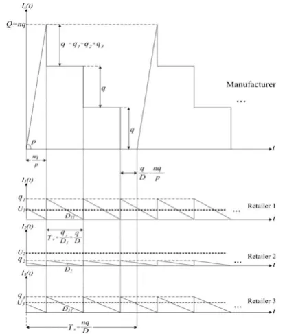
Consider a non-deteriorating single-item two-echelon single-manufacturer multi-retailer supply chain in which shortages aren’t allowed. The manufacturer produces inventory by constant rate . When on hand inventory at the manufacturer becomes a natural multiple of a total replenishment quantity of all the retailers ( ), the production is paused. At this moment, the manufacturer dispatches a total replenishment quantity ( ) to all the retailers instantaneously. As a result, the manufacturer’s inventory level decreases to ( ) and inventory level for each retailer increases by .
Based on VMI systems, it is assumed that the manufacturer replenishes the retailers at the same time. This is a reasonable assumption in VMI programs because the manufacturer makes decisions regarding the replenishment timing and amount. Each retailer consumes his inventory by constant rate . According to assumption of the simultaneous replenishment for all the retailers, inventory level for each of the retailers becomes zero at the same time. At this moment, the manufacturer dispatches the total replenishment quantity ( ) to all the retailers again instantaneously. This replenishment cycle is repeated until the manufacturer’s inventory level reaches zero. Afterwards, for ( ) time units, inventory level of the manufacturer remains zero and then by resuming the production at the rate , a new cycle for the manufacturer is started (Figure 1).
Figure 1. Inventory level against time for a single manufacturer and three retailers
While VMI can be implemented in conjunction with consignment, our paper focuses on non-consignment VMI setting in order to isolate impacts of the transfer of replenishment decisions to the manufacturer. Under non-consignment VMI environment, it is in the benefit of the manufacturer to push a lot of inventory downstream to save on the holding and dispatching costs. In order to prevent this trend, non-consignment VMI program includes contractual agreements between the manufacturer and each retailer. Under each contract, an upper bound is set on the retailer ’s inventory level such that the manufacturer pays a penalty cost per unit per unit time ( ) to this retailer for every unit of the retailer ’s inventory that is more than the upper bound .
The aim of this problem is to find optimal operating policies for the manufacturer and the retailers by considering the time value of money such that total annual cost of the whole supply chain is minimized.
4. MATHEMATICAL MODEL
4. 1. Assumptions and Notations The mathematical model in this research was developed on the basis of the following assumptions:
1) A two-echelon single-manufacturer multi-retailer supply chain with a non-deteriorating single-item under non-consignment VMI is considered. 2) Planning horizon is assumed to be infinite.
3) In order to take the time value of money into consideration, each of the inventory costs is discounted by a continuous compounding discount rate.
4) Demand and production rates are deterministic and constant.
5) The production rate is finite and greater than the sum of all retailers’ demand rates.
6) Shortages are not allowed. 7) The lead time is zero.
8) The manufacturer replenishes the retailers at the same time.
9) Each retailer can replenish more than once during the manufacturer’s cycle time.
10) There are no constraints on the capacity of warehouses, number of orders, production resources, and investment involved in inventory. 11) Based on VMI systems, it is assumed that the
manufacturer replenishes the retailers at the same time.
The following notations are used in the developed model:
: discount rate, : number of retailers,
: demand rate for retailer ,
∑ : total demand rate for all retailers, : setup cost per production run for manufacturer, : ordering cost for retailer per order,
: manufacturer’s holding cost per unit product per unit time,
: holding cost for retailer per unit product per unit time,
: over stock penalty cost for retailer per unit product per unit time,
: upper limit on the inventory level of retailer , : cycle time for retailer ,
: common cycle time of retailers, : manufacturer’s cycle time,
: replenishment quantity of retailer ,
∑ : total replenishment quantity of all retailers,
: number of shipments received by a retailer during the manufacturer’s cycle time,
: manufacturer’s production quantity, : set of all retailers whose upper limit is exceeded, ̅: set of all retailers whose upper limit is not exceeded (complement of the set ),
( ): manufacturer’s inventory level in terms of time, ( ): retailer ’s inventory level in terms of time, : equivalent annual ordering cost of retailer , : total equivalent annual ordering cost of all retailers,
: equivalent annual holding cost of retailer , : total equivalent annual holding cost of all retailers,
: equivalent annual setup cost of manufacturer, : equivalent annual holding cost of manufacturer, : equivalent annual penalty cost of manufacturer for violating the upper limit of retailer ,
: total equivalent annual penalty cost of manufacturer for violating the upper limits of all retailers,
: total equivalent annual cost of manufacturer, : total equivalent annual cost of retailer , : total equivalent annual cost of all retailers, : total equivalent annual cost of the whole supply chain,
: a very large positive number, and
: a binary variable equal to 1 if the retailer be a member of the set , and 0 otherwise.
4. 2. Modeling According to the simultaneous replenishment assumption for all the retailers we have:
* +
* + (1)
Based on Figure 1, the manufacturer’s cycle time will be:
(2)
According to Figure 1, the manufacturer’s inventory level in terms of time during the time interval * + is ( ) . So, in this interval, the manufacturer’s holding cost at time in a very small time interval can be obtained as follows:
(3)
By discounting this cost to time zero, the present value of Equation (3) will be:
(4)
By integrating Equation (4) on the time interval * +, the present value of the manufacturer’s holding cost during this interval is obtained as follows:
∫
(5)
According to Figure 1, the manufacturer’s inventory level in terms of time during the time interval *
+ is ( ) ( ) . As a result, in this interval, the present value of the manufacturer’s holding cost is calculated as follows:
∫ ( )
(6)
Hence, in the time interval * + (during the manufacturer’s cycle time), the present value of the manufacturer’s holding cost is:
∫
∑ ∫ ( )
( )
(7)
Considering infinite horizon, the present value of Equation (7) will be:
(∫
∑ ∫ ( )
( )
)
( ) (∫
∑ ∫ ( )
( )
) ∑
Also, considering infinite horizon, Equation (9) holds between the present value ( ) and equivalent annual value ( ) [23]:
(9)
Therefore, the equivalent annual value of the manufacturer’s holding cost is calculated according to Equation (10):
( ( (( ) ) (( ) ) ) ( (( ) )) ( ( ) ) ( (( ) ) ( ) )) ( ( (( ) ) ))
(10)
Always, th retailer’s inventory level in terms of time is ( ) ( ). For each retailer as a member of the set , the present value of the manufacturer’s penalty cost for violating the upper limit of retailer during the time interval * + is equal to:
∫ ( )
(11)
Therefore, during the time interval * +, the present value of Equation (11) will be:
(∫ ( )
) (
( )
) (∫ (
) ) ∑
(12)
Using the previous approach, the total equivalent annual penalty cost of the manufacturer is calculated in Equation (13):
∑ ∑ (∫ (
) ) ∑
∑
∑ ( (
) ( ) )
(
)
(13)
Considering the production setup cost at the beginning of the manufacturer’s cycle, equivalent annual value of this cost is obtained as follows:
∑
(
) (14)
If we consider the ordering cost for each retailer at the beginning of replenishment, the equivalent annual value of this cost for retailer will be:
∑
∑
(
) * +
(15)
The present value of holding cost for retailer during is:
∫ ( )
* +
(16)
Using the previous approach, the equivalent annual value of this cost will be:
(∫ ( )
) ∑
∑
( ( )) (
) * +
(17)
In both consignment and non-consignment VMI, the manufacturer incurs the retailers’ ordering cost. Also, unlike consignment VMI, in non-consignment VMI, each retailer incurs his holding cost. So, according to the problem under study, the manufacturer’s costs involved in this model are the retailers’ ordering cost, the manufacturer’s holding, setup, and penalty costs. Therefore, the total equivalent annual cost of the manufacturer under non-consignment VMI system is obtained from the following equation.
∑ ∑
(18)
Also, according to our problem, only cost incurred by each retailer is his holding cost. So, the equivalent annual cost of retailer will be:
* + (19)
Finally, the equivalent annual value of the total inventory cost for the whole supply chain will be resulted from the sum of Equations (18) and (19) as follows:
∑ (20)
Now, to model the proposed problem, we should consider Constraints (21) and (22):
(21)
They are included in order to ensure that penalty is incurred only for the retailers whose bound is violated. To decrease the number of variables of the model, we can rewrite Constraints (21) and (22) using Equation (1) as follows:
(23)
(24)
̅
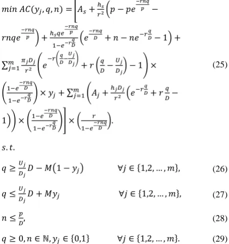
Now, the final model is formulated as a mixed integer non-linear programming (MINLP). The decision variables are , , and . We present this formulation below:
( ) [ (
)
(
)
∑ ( (
) ( ) )
(
) ∑ ( (
)) (
)] ( )
(25)
( ) * + (26)
* + (27)
(28)
* + * + (29)
The objective function (25) minimizes the total equivalent annual cost of the whole VMI supply chain. Constraint (26) is activated when . In this case, this constraint acts for members of the set according to relation (23).
Constraint (27) is activated when . In this case, this relation acts according to relation (24) for members of the set ̅. Constraints (26) and (27) ensure that penalty is incurred only for the retailers whose bound is violated. Constraint (28) ensures that shortages are not allowed (assumption 3); otherwise, according to relation (30), the manufacturing time ( ) will become
more than the common cycle time for retailers ( ) and they will face shortages.
( ( ))
(30)
5. SENSITIVITY ANALYSIS
In this section, a sensitivity analysis is conducted to study the effects of parameters on the optimal solution. In addition to performance description of the proposed model, this analysis also includes validation of the model. Unless specified otherwise, the model parameters are given below and in Table 1:
, , , and .
To study the effects of the parameter , we obtained optimal solutions for selected values of ranging from 0 to 24 with an increment of 4. The results are summarized in Table 2. Intuitively, from a continuous cash flow perspective, a holding cost is dependent on inventory levels at any time. So, when increases, it is better to decrease the manufacturer’s inventory level. Hence, value of decreases as increases according to Table 2.
TABLE 1. Parameters of retailers
Retailer
A 60 7 15 15 2
B 140 5 12 14 3
C 50 6 13 20 4
TABLE 2. Effect ofhs
s
h S Q n q ACVMI Tr Ts
VMI s
HC VMI
s
OC PCr VMI
r
OC VMI
r
HC
0 {B,A} 166.3 2 83.15 607.822 0.333 0.665 0 208.718 36.033 124.309 238.765
4 {B,A} 134.57 2 67.285 764.192 0.269 0.538 141.232 254.744 22.755 152.658 192.803
8 {B} 115.819 2 57.909 894.783 0.232 0.463 242.588 293.811 15.936 176.714 165.733
12 {B} 103.068 2 51.534 1008.92 0.206 0.412 323.352 328.504 11.632 198.074 147.363
16 {B,A} 76.955 1 76.955 1080.89 0.308 0.308 260.01 435.461 30.633 133.988 220.793
20 {B,A} 72.914 1 72.914 1144.11 0.292 0.292 307.732 458.856 27.249 141.186 209.089
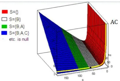
Surface in terms of and when and are represented in Figures 2 and 3, respectively. In and , the optimal solutions are depicted in red (Figure 2) and black points (Figure 3), respectively. Comparing these two surfaces shows the necessity of decrease in when increases. As increases, the state (Figure 2) has a much smaller increase in the objective function ( ) than the state (Figure 3). Moreover, as and decrease, the production runs and the manufacturer’s setup cost ( ) increase obviously.
It also seems that it is better to increase the total replenishment quantity ( ) when increases so that the manufacturer’s holding cost decreases. But, Table 2 shows that has a descending trend in equal values of . This is true because the decrease in the manufacturer’s penalty cost ( ) and the retailers’ holding cost ( ) not only compensates the increase in the manufacturer’s holding cost ( ) and the retailers’ ordering cost ( ), but also reduces the total cost of the VMI system ( ).
Figure 2. Surface in terms of and when
Figure 3. Surface in terms of and when
6. SUMMERY AND CONCLUSIONS
In the present research, we proposed a new model for a two-echelon single-manufacturer multi-retailer supply chain under non-consignment VMI and contractual agreements between the manufacturer and each retailer by considering the time value of money. Under this type of contracts, each retailer is protected by an upper bound on his inventory level, such that the manufacturer is penalized for quantity dispatched that is more than upper bound. In order to take the time value of money into consideration, the present value of each inventory cost was evaluated in a single period and generalized to infinity horizon and then transformed to the equivalent annual cost. Sensitivity analysis was conducted to study the effects of the parameters on the optimal solution and validate the proposed model. The most important results are presented as follows:
In case where penalty cost rate for a retailer is very low and the other one where upper bound of this retailer is high same optimal solutions exist. In both cases, the constraint related to upper bound on the retailer’s inventory will be redundant.
As penalty cost rate for a retailer is very high, the constraint related to over-stock limit of this retailer acts as a capacity constraint. This result can extend the proposed model in this paper to other applications where retailers have to manage the physical constraints of limited warehouse.
The sum of retailers’ ordering and holding costs and manufacturer’s penalty cost are nearly constant for different values of production rate.
As manufacturer’s production rate increases, the total replenishment quantity has a fluctuating behavior and the sensitivity of the optimal solution will become less. Also, when this rate is sufficiently large, the total annual cost of the whole system approaches to a value which is not dependent on it. The model can be further extended to some more practical situations, such as considering multi-manufacturer, multi-item and shortages, taking the raw material supply into account, and etc. We will consider these problems in the near future.
7. REFERENCE
1. Yao, Y., Dong, Y. and Dresner, M., "Managing supply chain backorders under vendor managed inventory: An incentive approach and empirical analysis", European Journal of
Operational Research, Vol. 203, No. 2, (2010), 350-359.
International Journal of Engineering-Transactions A: Basics, Vol. 27, No. 7, (2014), 1081-1090.
3. Akhbari, M., Zare Mehrjerdi, Y., Khademi Zare, H. and Makui, A., "A novel continuous knn prediction algorithm to improve manufacturing policies in a vmi supply chain", International
Journal of Engineering, Transactions B: Applications, Vol.
27, No., (2014), 1681-1690.
4. Guan, R. and Zhao, X., "On contracts for vmi program with continuous review (r, q) policy", European Journal of
Operational Research, Vol. 207, No. 2, (2010), 656-667.
5. Ahmadvand, A., Asadi, H. and Jamshidi, R., "Impact of service on customers' demand and members' profit in supply chain",
International Journal of Engineering, Vol. 25, No. 3, (2012),
213-222.
6. Hafezalkotob, A. and Makui, A., "Modeling risk of losing a customer in a two-echelon supply chain facing an integrated competitor: A game theory approach", International Journal of
Engineering, Vol. 25, No. 1, (2012), 11-34.
7. Clemmet, A., "Demanding supply", Work Study, Vol. 44, No. 7, (1995), 23-24.
8. Fry, M.J., Kapuscinski, R. and Olsen, T.L., "Coordinating production and delivery under a (z, z)-type vendor-managed inventory contract", Manufacturing & Service Operations
Management, Vol. 3, No. 2, (2001), 151-173.
9. Shah, J. and Goh, M., "Setting operating policies for supply hubs", International Journal of Production Economics, Vol. 100, No. 2, (2006), 239-252.
10. Darwish, M. and Odah, O., "Vendor managed inventory model for single-vendor multi-retailer supply chains", European
Journal of Operational Research, Vol. 204, No. 3, (2010),
473-484.
11. Woo, Y.Y., Hsu, S.-L. and Wu, S., "An integrated inventory model for a single vendor and multiple buyers with ordering cost reduction", International Journal of Production Economics, Vol. 73, No. 3, (2001), 203-215.
12. Zhang, T., Liang, L., Yu, Y. and Yu, Y., "An integrated vendor-managed inventory model for a two-echelon system with order cost reduction", International Journal of Production
Economics, Vol. 109, No. 1, (2007), 241-253.
13. Jasemi, M., "A vendor managed inventory", Master of Science Thesis, Department of Industrial Engineering, Sharif
University of Technology, Tehran, Iran (in Farsi), (2006),
115-123.
14. Nachiappan, S. and Jawahar, N., "A genetic algorithm for optimal operating parameters of vmi system in a two-echelon supply chain", European Journal of Operational Research, Vol. 182, No. 3, (2007), 1433-1452.
15. Sue-Ann, G., Ponnambalam, S. and Jawahar, N., "Evolutionary algorithms for optimal operating parameters of vendor managed inventory systems in a two-echelon supply chain", Advances in
Engineering Software, Vol. 52, (2012), 47-54.
16. Taleizadeh, A.A., Noori-daryan, M. and Cárdenas-Barrón, L.E., "Joint optimization of price, replenishment frequency, replenishment cycle and production rate in vendor managed inventory system with deteriorating items", International
Journal of Production Economics, Vol. 159, (2015), 285-295.
17. Pasandideh, S.H.R., Niaki, S.T.A. and Niknamfar, A.H., "Lexicographic max–min approach for an integrated vendor-managed inventory problem", Knowledge-Based Systems, Vol. 59, No., (2014), 58-65.
18. Sadeghi, J., Sadeghi, S. and Niaki, S.T.A., "Optimizing a hybrid vendor-managed inventory and transportation problem with fuzzy demand: An improved particle swarm optimization algorithm", Information Sciences, Vol. 272, (2014), 126-144. 19. Cachon, G.P. and Lariviere, M.A., "Contracting to assure
supply: How to share demand forecasts in a supply chain",
Management science, Vol. 47, No. 5, (2001), 629-646.
20. Yu, Y., Chu, F. and Chen, H., "A stackelberg game and its improvement in a vmi system with a manufacturing vendor",
European Journal of Operational Research, Vol. 192, No. 3,
(2009), 929-948.
21. Wong, W.-K., Qi, J. and Leung, S., "Coordinating supply chains with sales rebate contracts and vendor-managed inventory",
International Journal of Production Economics, Vol. 120, No.
1, (2009), 151-161.
22. Lee, J.-Y. and Cho, R.K., "Contracting for vendor-managed inventory with consignment stock and stockout-cost sharing",
International Journal of Production Economics, Vol. 151,
No., (2014), 158-173.
23. Çorbacıoğlu, U. and van der Laan, E.A., "Setting the holding cost rates in a two-product system with remanufacturing",
International Journal of Production Economics, Vol. 109, No.
Introducing the Time Value of Money in a Non-consignment Vendor Managed
Inventory Model
M. Parsaa, N. Mollaverdi-Esfahania, M. Alinaghianaa, R. Tavakkoli-Moghaddamb
a Department of Industrial and Systems Engineering, Isfahan University of Technology, Isfahan, Iran b School of Industrial Engineering, College of Engineering, University of Tehran, Tehran, Iran
P A P E R I N F O
Paper history: Received 15 May 2015
Received in revised form 09 April 2016 Accepted 14 April 2016
Keywords:
Vendor Managed Inventory Non-consignment Contractual Agreement Time Value of Money Sensitivity Analysis
ديكچ ه
( ُذٌشٍرف طسَت يدَجَه تيريذه
VMI
) راذيرخ يیب یگٌّاوّ يارب ِچراپکي درکيٍر کي
ىآ قبط ِک تسا ُذٌشٍرف
يیهأت( ُذٌشٍرف )ُذٌٌکذیلَت اي ُذٌٌک
يزاسرپزاب ِب طَبره تاویوصت ( راذيرخ
ُدرخ شٍرف ) یه راختا ار ذٌک شزرا لاحبات .
ٌِيسّ عَوجه یبايزرا رد لَپ یًاهز ُریجًز ياّ
تحت يیهأت ي
VMI
ِعلاطه رد ٍر ييا زا .تسا ُذشً ظاحل لذه کي رضاح ي
ُریجًز يارب ذيذج ُدرخ ذٌچ ٍ ُذٌٌکذیلَت کي اب یحطسٍد يیهأت ي
ِهاًرب تحت شٍرف ي
VMI
يتفرگ رظًرد اب یتًاهاریغ
یه ِئارا لَپ یًاهز شزرا َش
.د ِب ٌِيسّ یلعف شزرا اذتبا لَپ یًاهز شزرا ىدرک دراٍ رَظٌه ٍ ِبساحه ُرٍد کي یط رد اّ
ٌِيسّ ِب ذعب ٍ نیوعت تياًْ یب قفا ِب سپس یه ليذبت ًِایلاس گٌسوّ ي
ش ِب لذه ييا يیٌچوّ .دَ صخشه رَط
تقفاَه ِهاً ُدرخ رّ ٍ ُذٌٌکذیلَت يیب يدادرارق ياّ یه لهاش ار شٍرف
حت .دَش حطس يٍر لااب ذح کي اّدادرارق عًَ ييا ت
ُدرخ يدَجَه یه يییعت شٍرف
ِب دَش يرَط یه زٍاجت ذح ييا زا ِک یلَصحه ذحاٍ رّ يارب ُذٌٌکذیلَت ِک ِويرج ،ذٌک
یه ِعلاطه يارب تیساسح سیلاًآ ىاياپ رد.دَش یه ماجًا لذه يزاسربتعه ٍ ٌِیْب باَج يٍر يذیلک ياّرتهاراپ ریثأت ي
.دَش