TWO STAGE MULTIPLE ATTRIBUTE DECISION MAKING
PROBLEM IN IRANIAN GAS DISTRIBUTION SYSTEMS
M. B. Aryanejad
Faculty of Industrial Engineering, Iran University of Science and Technology Tehran, Iran, [email protected]
S. Ghavampour
Research and Science Branch, Iran Azad University Tehran, Iran, [email protected]
(Received: June 22, 2002 – Accepted in Revised Form: December 24, 2003)
Abstract The purpose of this paper is to present the possibility of replacing physical unit cost in transportation or distribution problems by an aggregate coefficient, getting qualitative and subjective considerations involved. The model for constructing aggregate cost is a two stage multiple attribute decision-making problems. In the first stage supply points, demand points and routes of transportation are alternatives and have to be weighted against their own attributes. In the second stage, the alternatives are placed as attributes in a new matrix and the unit aggregate costs will be the new alternatives. Some heuristic techniques are developed for tradeoffs between attributes. Experts and decision-makers do tradeoff. The results are compared with the simple physical costs.
Key Words Aggregate Cost, Multiple Attributes, Distribution
ﻩﺪﻴﻜﭼ
ﻩﺪﻴﻜﭼ
ﻩﺪﻴﻜﭼ
ﻩﺪﻴﻜﭼ
ﻑﺪﻫ ﻦﻳﺍ ﻪﻟﺎﻘﻣ ﺔﺋﺍﺭﺍ ﺞﻳﺎﺘﻧ ﻖﻴﻘﺤﺗ ﺭﺩ ﺩﺭﻮﻣ ﻲﻨﻴﺸﻧﺎﺟ ﻞﻣﺎﻋ ﻪﻨﻳﺰﻫ ﺭﺩ ﻞﺋﺎﺴﻣ ﻞﻤﺣ ﻭ ﻞﻘﻧ ﻳﺯﻮﺗﻭ ﻊ ﺎﺑ ﻚﻳ ﺐﻳﺮﺿ ﻲﻣﺎﻏﺩﺍ ﺖﺳﺍ ﻪﻛ ﻩﻭﻼﻋ ﺮﺑ ﺔﻨﻳﺰﻫ ﻲﻜﻳﺰﻴﻓ ﺕﺎﻈﺣﻼﻣ ﻱﺮﻈﻧ ﻭ ﺖﻳﺩﻭﺪﺤﻣ ﻱﺎﻫ ﺹﺎﺧ ﻊﺑﺎﻨﻣ ، ﻁﺎﻘﻧ ﻑﺮﺼﻣﻴﻧ ﺍﺭ ﻊﻳﺯﻮﺗﻱﺎﻫﺮﻴﺴﻣﻭ ﺰ ﻅﻮﺤﻠﻣ ﺪﻳﺎﻤﻧ . ﺭﺩ ﻦﻳﺍ ﺵﻭﺭ ﻞﻣﺎﻋ ﻪﻨﻳﺰﻫ ﺪﺣﺍﻭ ﻤﺣ ﻞ ﻭ ﻞﻘﻧ ﻪﻛ ﺭﺩ ﻱﺎﻬﺷﻭﺭ ﻲﻠﻌﻓ ﻲﻠﻣﺎﻋ ﻦﻴﻴﻌﺗ ﻩﺪﻨﻨﻛ ﺭﺩ ﻪﻨﻴﻬﺑ ﻱﺯﺎﺳ ﻊﻳﺯﻮﺗ ﻲﻣ ﺪﺷﺎﺑ ﻱﺎﺟ ﺩﻮﺧ ﺍﺭ ﻪﺑ ﺔﻨﻳﺰﻫ ﻲﻣﺎﻏﺩﺍ ﻲﻣ ﺪﻫﺩ . ﻡﺎﻤﺗ ﺕﺎﻈﺣﻼﻣ ﻲﻔﻴﻛ ﻱﺍﺮﺑ ﻊﺑﺎﻨﻣ ، ﻁﺎﻘﻧ ﻑﺮﺼﻣ ﻭ ﺰﻴﻧ ﺮﻴﺴﻣ ﻞﻤﺣ ﻭ ﻞﻘﻧ ﺩﺍﻮﻣ ﺭﺩ ﻦﻳﺍ ﺔﻨﻳﺰﻫ ﻲﻣﺎﻏﺩﺍ ﺭﻮﻈﻨﻣ ﻲﻣ ﺩﺩﺮﮔ . ﻦﻳﺍ ﻪﻨﻳﺰﻫ ﻲﻌﻗﺍﻭ ﺮﺗ ﺯﺍ ﺔﻨﻳﺰﻫ ﻲﻟﻮﻤﻌﻣ ﺖﺳﺍ ﺍﺮﻳﺯ ﺰﻫ ﻪﻨﻳ ﻱﺎﻫ ﺖﺻﺮﻓ ﻭ ﻪﻨﻳﺰﻫ ﻱﺎﻫ ﻲﺟﺭﺎﺧ ﺍﺭ ﻪﺑ ﻲﺑﻮﺧ ﺲﻜﻌﻨﻣ ﻲﻣ ﺪﻨﻛ . ﺩﺮﺑﺭﺎﻛ ﻦﻳﺍ ﻪﻨﻳﺰﻫ ﺭﺩ ﻞﺣ ﻞﺋﺎﺴﻣ ﻊﻳﺯﻮﺗ ﻪﺑ ﻱﺎﻬﺑﺍﻮﺟ ﻲﻌﻗﺍﻭ ﻱﺮﺗ ﺮﺠﻨﻣ ﻲﻣ ﺩﺩﺮﮔ . ﻝﺪﻣ ﺕﺭﺎﺒﻋ ﺖﺳﺍ ﺯﺍ ﻚﻳ ﺔﻠﺌﺴﻣ ﻢﻴﻤﺼﺗ ﻱﺮﻴﮔ ﺪﻨﭼ ﺓﺭﺎﻴﻌﻣ ﻭﺩ ﻪﻠﺣﺮﻣ ﻱﺍ . ﺵﻭﺭ ﻭﺩ ﻪﻠﺣﺮﻣ ﻱﺍ ﻦﻳﺍ ﺖﺻﺮﻓ ﺍﺭ ﻲﻣ ﺪﻫﺩ ﻪﻛ ﺭﺎﻴﻌﻣ ﻱﺎﻫ ﻲﻔﻴﻛ ﻊﺑﺎﻨﻣ ، ﻁﺎﻘﻧ ﺼﻣ ﻑﺮ ﻭ ،ﺮﻴﺴﻣ ﻪﻧﺎﮔﺍﺪﺟ ﻭ ﻂﺳﻮﺗ ﻥﺎﺳﺎﻨﺷﺭﺎﻛ ﻭ ﻢﻴﻤﺼﺗ ﻥﺍﺮﻴﮔ ﻁﻮﺑﺮﻣ ﺩﺭﻮﻣ ﻲﺑﺎﻳﺯﺭﺍ ﺭﺍﺮﻗ ﻴﮔ ﺩﺮ . . ﻪﻨﻳﺰﻫ ﻱﺎﻫ ﻲﻣﺎﻏﺩﺍ ﻞﺻﺎﺣ ﻦﻳﺰﮕﻳﺎﺟ ﻪﻨﻳﺰﻫ ﻱﺎﻫ ﻲﻟﻮﻤﻌﻣ ﺭﺩ ﺕﻻﺩﺎﻌﻣ ﻪﻨﻴﻬﺑ ﻱﺯﺎﺳ ﻞﺋﺎﺴﻣ ﻊﻳﺯﻮﺗ ﻲﻣ ﺪﻧﺩﺮﮔ . ﻪﺠﻴﺘﻧ ﻥﺎﺸﻧ ﻲﻣ ﺪﻫﺩ ﻪﻛ ﻪﻨﻳﺰﻫ ﻱﺎﻫ ﺎﺑﻲﻣﺎﻏﺩﺍ ﻪﻨﻳﺰﻫ ﻱﺎﻫ ﻲﻟﻮﻤﻌﻣ ﻑﻼﺘﺧﺍ ﻞﺑﺎﻗ ﻪﺟﻮﺗ ﺪﻧﺭﺍﺩ ﻭ ﺩ ﺭ ﻱﺭﺎﻴﺴﺑ ﺩﺭﺍﻮﻣ ﻪﺑ ﺦﺳﺎﭘ ﻱﺎﻫ ﻒﻠﺘﺨﻣ ﺮﺠﻨﻣ ﻲﻣ ﺪﻧﻮﺷ . 1. INTRODUCTION
The unit cost in classical transportation, distribution design and facility location have been the sole dominant in finding optimal solution for many years of academic works and project implementation. In this paper we are focused on qualitative aspects of supply, demand zones and routes. These together with the physical cost of transportation will be our new criteria for finding optimal way of source allocation or distribution problems. A two stage
content requirements in distribution systems and Wlodzimierz Ogryczak [2] have incorporated qualitative aspects of cost element in location and distribution problems. Frank Plasteria [3] has suggested consumer utilities as a criterion to be also considered in distribution problem other than cost. All of these endeavors are symptoms of necessity for considering qualitative aspects of supply, demand points and routes. In this paper all major qualitative factors are fed to the model for considering the increasing needs for attention to fast changing economy, environment and technology. Carrizosa and Conde [4] in their locating model assume the cost as a function of the network distances to users. But in an extension they use Weber’s problem to locate a facility in the Euclidean plane in order to minimize the sum of its (weighted) distances to the locations of a given set of users.
Pino et al. [5] have estimated a system of equations for distance function and cost shares and consider labor and capital as cost criteria. In the production-distribution models, Dasci and Verter [6] show that a few researchers have employed various extrinsic criteria for decision-making. Of course only some of important factors have been considered. In the mathematical models and operations research textbooks the sources and destinations with high or low priority are given a big or small cost value to be considered properly in decision-making. In this paper we have assumed the cost not only as a function of distance but also a function of all major extrinsic variables like technology, government policy and environmental impacts.
The paper has been organized in five sections. The first section is devoted to introducing TSMADM.
In second section the new aggregate cost element is formulated. Calculation for aggregate costs will be presented in section three through an example. In section four related models are compared. The conclusion will be presented in section five.
2. TWO STAGE MULTIPLE ATTRIBUTE DECISION MAKING
In many cases in transportation and distribution problems, suppliers that have to cover planned demands, have not the same qualitative levels. The demand zones also differs when qualitative parameters are taken into account. These differences are crucial to decision makers when hard policies have to be considered for allocating sources to demand points.
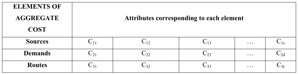
Qualitative decision making elements for supply zones, demand areas and the routes between are shown in Table 1. This is a three element aggregate cost concept.
For each alternative of distributing supply to demand points there are (s+d+r) criteria. The proposed method takes these criteria as the components of aggregate qualitative cost. Sources, demand points and routes are the first stage alternatives. They are ranked against their own criteria. The second stage alternatives, which are various competitors for supplying individuale demand points, are compared based on above-mentioned three main elements of aggregate qualitative cost. In the next section we formulate the method. We have to notice that this method differs from AHP [7] because each of the first stage alternatives (for example various sources) has its own attributes TABLE 1. Aggregate Cost Concept.
ELEMENTS OF AGGREGATE
COST
Attributes corresponding to each element
Sources C11 C12 C13 … C1s
Demands C21 C22 C23 … C2d
which are not applicable for the others. In other words the attributes are not common for all alternatives to allow us for constructing hierarchical system.
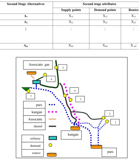
Therefore in the second stage of problem we have a number of possible choices each containing one supply point, one demand point and a proposed route between.
TABLE 2. The Second Stage MADM.
Second stage attributes Second Stage Alternatives
Supply points Demand points Routes
A1 X11 X12 X13
A2 X21 X22 X23
… … … …
Am Xm1 Xm2 X m3
refinery
source demand
pars kangan
Associate gas
1 2 3
4 5
6
7
pars
Associate kangan
shared
3. TWO STAGE MADM FORMULATION
After incorporating MADM proper methods for each row in Table 1, the first stage of solution is terminated and each of three sets of alternatives are ranked.We have usedpair wise comparison matrix to assess the relative contribution of supply and demand alternatives for each related attribute. In the second stage for each alternative the number of criteria is three: supply, demand and route. Table 2 shows the second stage of MADM problem. Contribution of alternatives for each related attribute would be available by use of pair wise comparison matrix. The next step is to link quantitative data to physical cost of each second stage alternative so that we could add qualitative and quantitative figures to each other. Selecting an attribute, which is better exchanged to quantitative figures, should do this. The quantitative values of other attributes are proportionally calculated based on comparative data. A better way is to refer to the first stage attributes to find which are more tangible and changeable to quantitative figures.
This will be clear in the following example.
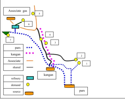
4. AN APPLICATION EXAMPLE
Figure 1 shows a distribution system for supplying natural gas to demand points in south of Iran. There are 3 supply points (Pars, Nar and Kangan, Associated gas field), 7 demand points (Southeast, Jahrom, Shiraz, Central and Western, Esfahan, Northwest export and injection in Aghajari) and 12 transportation routes involved in the natural gas distribution among selected areas.
Tables 3 and 4 show the attributes of sources and demand points respectively and evaluated numbers for them. The values have been calculated based on the results of two questionnaires prepared for the job. The questionnaires on supply and demand were designed for getting comments from decision makers through subjective pair wise comparisons. The weight of each first stage attributes can be calculated through eigenvector method.
TABLE 3. Pairwise Comparisons Between Supply Attributes.
Development Environment Byproducts Urgency
Development 1 2 1/2 1/3
Environment 1/2 1 1/3 1/5
Byproducts 2 3 1 1/2
Urgency 3 5 2 1
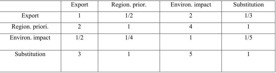
TABLE 4. Pairwise Comparisons Between Demand Attributes.
Export Region. prior. Environ. impact Substitution
Export 1 1/2 2 1/3
Region. priori. 2 1 4 1
Environ. impact 1/2 1/4 1 1/5
Only one qualitative attribute has been considered for routes in this example.
The quantitative attribute for distribution system is cost per one cubic meter of natural gas distributed to demanders. This includes production, refining, transmission and distribution costs. The four major qualitative attributes for supply areas are: development level [8], environment protection requirements, by products recovery and urgent on gas withdrawal. The demand attributes are: regional priorities, environment protection requirements [9], export potential and substitution advantages and the criterion for routes is environment protection requirements. For supply and demand attributes the pair wise comparisons have been done through questionnaires answered by experts and shown in Tables 3 and 4. The λmax values by using eigenvector method for these tables are 4.01 And 4.02 respectively and the weights of the attributes for supply and demand are as follows: Ws = (0.157, 0.088, 0.272, 0.483) and Wd = (0.158, 0.35, 0.083, 0. 41).
Tables 5 and 6 show comparisons of supply and
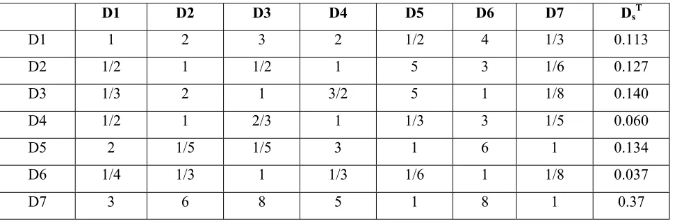
demand points with respect to one of their relative attributes. The results of comparisons are put in two vectors: SdT = (0.56, 0.32, 0.12) for supply and DsT = (0.113, 0.127, 0.14, 0.08, 0.134, 0.037, 0.37) for demand. The same calculation is done for the other attributes.
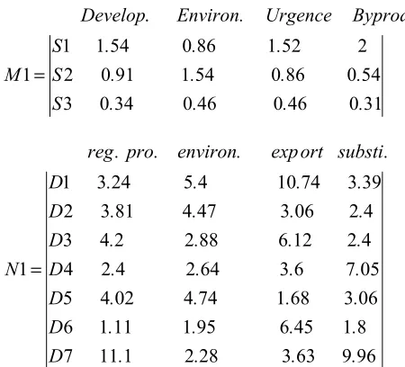
The results for the other attributes can be viewed in matrices M and N.
The first column of matrix M, stands for development attribute and so on. This is the same for matrix N and demand attributes. Matrix O, stands for routes single criteria.
It worth to mention that each column is obtained by judgments from experts and DM’s directly engaged in the subject. It is one of the advantages of this method.
11 0 16 0 16
0 12 0 3
19 0 3 0 54
0 32
0 2
7 0 54 0 3
0 56
0 1
.
99 2 1
3 0
3 36
3
. .
. .
S
. .
. .
S
. .
. .
S M
. Byprod Urgence
. Environ Develop
. .
. .
. max
= = λ
TABLE 5. Comparison of Supply Points with Respect to Development Potential.
S1 S2 S3 SdT
S1 1 2 4 0.56
S2 1/2 1 3 0.32
S3 1/2 1/3 1 0.12
TABLE 6. Comparison of Demand Points with Respect to Substitution Potential.
D1 D2 D3 D4 D5 D6 D7 DsT
D1 1 2 3 2 1/2 4 1/3 0.113
D2 1/2 1 1/2 1 5 3 1/6 0.127
D3 1/3 2 1 3/2 5 1 1/8 0.140
332 0 121 0 076 0 37 0 7
06 0 215 0 065 0 037 0 6
102 0 056 0 158 0 134 0 5
235 0 120 0 088 0 08 0 4
08 0 204 0 096 0 14 0 3
08 0 102 0 149 0 127 0 2
108 0 18 0 358 0 113 0 1
24 9 02 8 22
7 16
7
. .
. .
D
. .
. .
D
. .
. .
D
. .
. .
D
. .
. .
D
. .
. .
D
. .
. .
D
N
. environ ort
exp . substi .
pro . reg
. .
. .
. max
= =
λ O = (R1, R2, R3, R4, R5, R6, R7, R8, R9, R10,
R11, R12) = (0.3, 0.065, 0.06, 0.06, 0.095, 0.034, 0.07, 0.055, 0.05, 0.066, 0.05, 0.085)
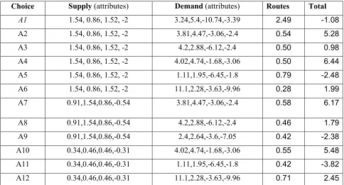
In matrices M and N and O, the figures for attributes are comparative and need to be comparable with quantitative unit cost of distribution network. For each matrix the candidate attribute that is better changed to quantities is selected. For supply, by products and for demand, substitution is the best. Also for each of these two criteria the more suitable TABLE 7. Decision Matrix for Determining Aggregate Qualitative Cost.
Choice Supply (attributes) Demand (attributes) Routes Total
A1 1.54, 0.86, 1.52, -2 3.24,5.4,-10.74,-3.39 2.49 -1.08
A2 1.54, 0.86, 1.52, -2 3.81,4.47,-3.06,-2.4 0.54 5.28
A3 1.54, 0.86, 1.52, -2 4.2,2.88,-6.12,-2.4 0.50 0.98
A4 1.54, 0.86, 1.52, -2 4.02,4.74,-1.68,-3.06 0.50 6.44
A5 1.54, 0.86, 1.52, -2 1.11,1.95,-6.45,-1.8 0.79 -2.48
A6 1.54, 0.86, 1.52, -2 11.1,2.28,-3.63,-9.96 0.28 1.99
A7 0.91,1.54,0.86,-0.54 3.81,4.47,-3.06,-2.4 0.58 6.17
A8 0.91,1.54,0.86,-0.54 4.2,2.88,-6.12,-2.4 0.46 1.79
A9 0.91,1.54,0.86,-0.54 2.4,2.64,-3.6,-7.05 0.42 -2.38
A10 0.34,0.46,0.46,-0.31 4.02,4.74,-1.68,-3.06 0.55 5.48
A11 0.34,0.46,0.46,-0.31 1.11,1.95,-6.45,-1.8 0.42 -3.82
A12 0.34,0.46,0.46,-0.31 11.1,2.28,-3.63,-9.96 0.71 2.45
TABLE 8. Results of Second Stage MADM.
Alternative A1 A2 A3 A4 A5 A6 A7 A8 A9 A10 A11 A12
Qualitative cost -1.08 5.28 0.98 6.4
4 -2.5 2
6.1
7 1.8 -2.4 5.48 -3.82 2.45
Physical cost 7 6.5 6 5.5 7.5 7 6.8 7.1 6.9 5 7.2 6.8
supply point and demand zone are identified. S1 (Pars field) and D3 (Shiraz) are the best. In this case routes criterion is changed to quantities regarding environmental attributes of supply and demands. The byproducts value for Pars field are evaluated about 2 cent per cubic meter of produced natural gas and the Shiraz substitution benefit is around 2.4 cent/M3. These two figures are corresponding to 0.7 and 0.08 in matrices M and N. Proportionally all other values in matrices are changed to money (matrices M1, N1 and O1). Environmental requirements for the route in choice A3 is estimated around 0.5 cent/M3 transported gas. Table 7 shows the new values of alternatives via 12 different choices.
31 0 46 0 46 0 34 0 3 54 0 86 0 54 1 91 0 2 2 52 1 86 0 54 1 1 1 . . . . . S . . . . S . . . S M . Byprod Urgence . Environ Develop = 96 9 63 3 28 2 1 11 7 8 1 45 6 95 1 11 1 6 06 3 68 1 74 4 02 4 5 05 7 6 3 64 2 4 2 4 4 2 12 6 88 2 2 4 3 4 2 06 3 47 4 81 3 2 39 3 74 10 4 5 24 3 1 1 . . . . D . . . . D . . . . D . . . . D . . . . D . . . . D . . . . D N . substi ort exp . environ . pro . reg =
O1 = (R1, R2, R3, R4, R5, R6, R7, R8, R9, R10,
R11, R12) = (2.49, 0.54, 0.5, 0.5, 0.79, 0.28, 0.58, 0.46, 0.42, 0.55, 0.42, 0.71)
The net result of supply, demand and routes attributes tradeoff is added to unit cost of each distribution choice (Table 7). It is worth to mention that A1 to A12 are the second stage alternatives. This vector takes the role of unit cost in transportation and distribution problems where subjective attributes on start and end points and the routes are important for decision makers.
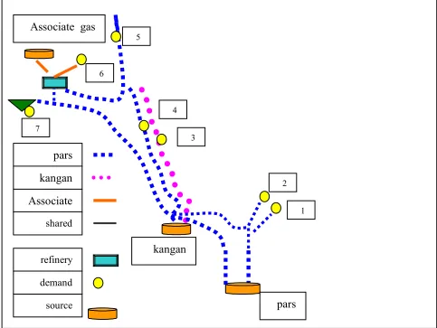
per day of natural gas and equal to S = (125,90,30) and D=(25,27,42,47,20,30,50). The unit costs are as in table 8. In Figure 3 (based on physical cost) the rejected alternatives are (A2, A4, A9), while for the case of aggregate cost (Figure 4) the removed alternatives will be (A3, A5, A7, A10, A12).
5. COMPARISON
The models applied for distribution problems have not been focused on the nature of large-scale industries when long-term consideration is of high importance. The extrinsic criteria are essential for allocating sources between various consumers. In
some of these models only part of extrinsic criteria have been considered like price uncertainty, tariffs and exchange rate uncertainty.
Priority policy involved in the model has been implied in many industries like power plants, oil and gas industry. Applying two-stage model has its merit for easing problem solving when compared with models dealing with a large number of attributes and demanding sophisticated mathematical method with high possibility of error.
The system dynamics methods [10]can be applied to construct the aggregate cost curves for long term considerations. The weakness of this method will be prediction formulation errors.
The most important disadvantage of TSMADM is that the collecting data will be time consumer because more experts have to be interviewed for refinery
source demand
pars kangan
Associate gas
1 2 3
4 5
6
7
pars
Associate kangan
shared
subjective information.
6. CONCLUSION
The existence of hidden effects of long term and macroeconomic parameters on decisions taken for selecting the best distribution pattern justifies that the aggregate costs is more reliable than physical costs especially when we are going to set a long term planning. It means that in a number of alternatives the external impacts are important and may affect the decisions accuracy. A part of post optimality analysis for distribution problems will be conducted
through incorporating two stages MADM model by changing or altering attributes without affecting the main structure of optimization models formulation.
Considering supply, demand and routes as separate fields of expertise help us to get the best results for comparisons on attributes or weighting alternatives. The number of attributes shrinks significantly because of breaking the decision in two stages. In the example we have comparisons in groups with maximum 4 attributes instead of a comparison between 9 attributes. In large-scale problems this advantage will be more highlighted. In energy section, the extrinsic aspects of supply demand points and routes are more controversial refinery
source demand
pars
kangan
Associate gas
1 2 3
4 5
6
7
pars
Associate
kangan
shared
than the cost of physical installations. The method has considered this case in its best way.
One strength point of the paper is making tradeoffs with cost which is tangible for supply and demand experts and DM’s. The breakdown to attributes has made tradeoffs with cost more meaningful than trading off the supply and demand levels directly with cost.
This study makes clear the concept of Extrinsic Values [11] for commodities like natural gas, which are not renewable and stored in different geographical location. The opportunity cost of supplying commodities to demanders will also be clarified.
7. REFERENCES
1. Arntzen, B. C., Brown, G. G. and Harrison, T. P., “Global Supply Chain Management at Digital Equipment Corporation”, Interfaces 25, (1995), 69-93.
2. Wlodzimierz and Ogryczak, “Quality Measures and Equitable Approaches to Location Problems”, European Journal of Operational Research, 122, (2000), 374-391. 3. Plasteria, F., “Static Competitive Facility Location:
An Overview of Optimization Approaches”, European
Journal of Operational Research, 129, (2001), 461-470.
4. Carizosa and Conde, “A Fractional Model for Locating
Semi-Desirable Facilities on Networks”, European
Journal of Operational Research, Vol. 136, (1), (Jan. 2002), 67-80.
5. Pino, J. B., Blanco, V. F. and Alvarez, A. R. “The Allocative Efficiency Measure by Means of a Distance Function: The Case of Spanish Public Railway”,
European Journal of Operational Research, Vol. 137, No. 1, (2002), 191-205.
6. Dasci, A. and Verter, V., “An Application of DEA fo r Comparative Analysis and Ranking of Regions in Serbia with Regards to Social-Economic Development”, European Journal of Operational Research, Vol. 132, (2), (16 July 2001), 343-356.
7. Hwang, C. L. and Yoon, K., “Analytical Hierarchical Process”, Lecture Notes in Economics and Mathematical System, MADM, Methods and Applications, Hwang and Lee, (1972), 41-43.
8. Odone and Bebbington, BP Exploration(Alaska) INC., External Affairs Department, Online Address: http:// www.bp.com, (2001).
9. P u zak, J. , “Decisio n M akin g an d V al u at i o n fo r En viro n men tal P o licy”, On lin e Ad d ress: http:// es.epa.gov/ ncer/rfa/ 98valrfa.html, (1998).
10. Sterman, J., http://web.mit.edu/jsterman/www/BusDyn2. html#Features_and_Content.