International Journal of Engineering Vol. 18, No. 1, February 2005 -1
SOLUTION OF FLOW FIELD EQUATIONS AND VERIFICATION
OF CAVITATION PROBLEM ON SPILLWAY OF THE DAM
S. A. Mirbagheri
Department of Civil Engineering, K. N. Toosi University of Technology, Tehran, IRAN
M. N. Mansouri
Graduate Student in Hydraulic Structure
(Received: jan. 24, 2003 – Accepted in Revised Form: Aug. 4, 2005)
Abstract The main objective of this paper is to formulate a mathematical model for finding flow field and cavitation problem on dam spillways. The Navier-Stokes Equation has been applied for the computation of pressure and velocity field, free water surface profiles and other parameters. Also, for increasing accuracy of the problem, viscosity effect has been considered. Because of internal flows the effect of gravity forces has been ignored. To have more accuracy the continuity and momentum equations have been transformed to a coordinate system with axis tangent and normal to stream flow.
Finite differences has been used to solve equations governing the over flow of dam the spillways. To linearize the nonlinear equations the parameters are expressed in terms of products of last step in the new one. Later the remaining derivatives are with finite differences form. Coefficients of convergence as well as a three diagonal system are used for all the grids points. The cavitation phenomena are discussed after determination of velocity and pressure fields, which cause erosion on the spillway shut and side walls. Also, the different types of cavitations and appropriate solutions were considered and a computer program <MANS> was developed Two examples were solved on this basis and the computed results were compared with experimental results. The results show that for flows up to 4000 m3/sec the condition is good, but for flows higher than this value, the water surface shows high uprising and provisions are needed to resist cavitation at these flows. The results also indicate that at flows about 10899 m3/sec secondary flows dominate near the lateral gates and side walls.
Key Words Solution of Flow Field, Equation, Cavitation, Spillway, Dam, Finite Difference
ﺪﻴﻜﭼ ﻩ
ﻩﺪـﻳﺪﭘﻦﻴـﻴﻌﺗونﺎـﻳﺮﺟناﺪـﻴﻣندروﺁﺖـﺳﺪﺑﺖـﻬﺟﯽﺿﺎﻳرلﺪﻣدﺎﺠﻳا،ﻪﻟﺎﻘﻣﻦﻳاﯽﻠﺻافﺪه
ﺪﺷﺎﺑﯽﻣﺪﺳﺰﻳرﺮﺳﯼورﺮﺑﯽﻳادزﻩﺮﻔﺣ
. ﻪﻟدﺎﻌﻣ ﺮﻳوﺎﻧ ﺲﮐﻮﺘﺳا
ناﺪـﻴﻣﻦﻴـﻴﻌﺗﺖـﻬﺟ
رﺎﺸـﻓ
،
ﺖﻋﺮـﺳ
ونﺎﻳﺮﺟ ﻞﻴﻓوﺮﭘ
ﺖـﻗدندﺮـﺑﻻﺎـﺑﯼاﺮـﺑﺎﻨﻤـﺿ؛ﺪـﻣﺁﺖﺳﺪﺑﺰﻳرﺮﺳﯼورﺮﺑﺎهﺮﺘﻣارﺎﭘﺮﻳﺎﺳوبﺁدازﺁﺢﻄﺳ
ﻞﻤﻋ ،
ﺪﺷﻪﺘﻓﺮﮔﺮﻈﻧردلﺎﻴﺳﺖﺟﺰﻟ
.
ﺪـﺷﻪﺘﻓﺮﮔﻩﺪﻳدﺎﻧنﺎﻳﺮﺟﺖﻴﻌﺿوﻞﻴﻟدﻪﺑﻞﻘﺛﯼوﺮﻴﻧﺮﺛا
. ﻪـﻟدﺎﻌﻣ
وﻪﺘﺳﻮﻴﭘنﺎﻳﺮﺟ ﻢﺘﻨﻤﻣ
لﺎﻣﺮﻧنﺎﻳﺮﺟﺮﻴﺴﻣردتﺎﺼﺘﺨﻣﻩﺎﮕﺘﺳدﮏﻳردار
شورﺎـﺑ
ﯼﺎـهتوﺎـﻔﺗ
دوﺪـﺤﻣ
ﺪﺷﻞﺣ
. بﺮـﺿﻞﺻﺎﺣسﺎﺳاﺮﺑارﺎهﺮﺘﻣارﺎﭘ،ﯽﻄﺧﺮﻴﻏتﻻدﺎﻌﻣندﺮﮐﯽﻄﺧﯼاﺮﺑ مﺮـﺗ
ردﻢﻳﺪـﻗﯼﺎـه
ﺪﺷنﺎﻴﺑﺪﻳﺪﺟ
.
ﺪـﺷﻪـﺘﻓﺮﮔﺮـﻈﻧردطﺎـﻘﻧمﺎـﻤﺗﯼاﺮـﺑ،ﯼﺪـﻌﺑﻪﺳﻢﺘﺴﻴﺳردﯽﻳاﺮﮕﻤهﺐﻳﺮﺿ
. زاﺪـﻌﺑ
ﻩﺪﻳﺪﭘنﺎﻳﺮﺟﺖﻋﺮﺳورﺎﺸﻓناﺰﻴﻣﻦﻴﻴﻌﺗ
ردﺶﻳﺎـﺳﺮﻓﺚـﻋﺎﺑﻪـﮐﯽـﻳازﻩﺮـﻔﺣ
راﻮـﻳدوﺮﺘﺴـﺑ ﻩ
ﺎـه
ﯽـﻣ
،دﻮﺷ
ﺖﻓﺮﮔراﺮﻗﺚﺤﺑدرﻮﻣ
.
ﺪـﻳدﺮﮔﻪـﻳارانﺁلﺮﺘﻨﮐﯼﺎهشوروﯽﻳازﻩﺮﻔﺣﻩﺪﻳﺪﭘعاﻮﻧاﻦﻴﻨﭽﻤه
. ﺎﻨﻤـﺿ
ناﻮﻨﻋﺖﺤﺗﯼﺮﺗﻮﻴﭙﻣﺎﮐﻪﻣﺎﻧﺮﺑﮏﻳ
MANS
تﻻدﺎﻌﻣﻞﺣﯼاﺮﺑ
ﺪـﺷﻪـﺘﻓﺮﮔرﺎـﮐﻪـﺑوﻪﺘﺷﻮﻧ
. ﻞـﺣلﺎـﺜﻣود
ارلﺪﻣﻂﺳﻮﺗﻩﺪﺷﻪﺒﺳﺎﺤﻣﺞﻳﺎﺘﻧوﺪﺷ ﺑ،
ﺪﺷﯼﺮﻴﮔﻩزاﺪﻧامﺎﻗراﺎ
،ﺪﺷﻪﺴﻳﺎﻘﻣﻩ
زاﻩﺪﻣﺁﺖﺳﺪﺑﺞﻳﺎﺘﻧ
لﺪﻣ
MANS نﺎﻳﺮﺟﺎﺗﻪﮐﺪهدﯽﻣنﺎﺸﻧ
4000
ﻩﺪـﺷﻪﺒـﺳﺎﺤﻣمﺎـﻗرا،ﻪـﻴﻧﺎﺛﺮﺑﺐﻌﮑﻣﺮﺘﻣ
ﻩﺪهﺎﺸـﻣﺎـﺑ
ﻩﺪﺷ
ﻦـﻳازاﺮﺘﺸـﻴﺑﯼﺎـهنﺎـﻳﺮﺟﯼاﺮﺑﯽﻟو،ﺪﻧرادﯽﺑﻮﺧﯽﻧاﻮﺨﻤه ﯽـﺗاﺮﻴﻴﻐﺗ
دﻮـﺟﻮﺑبﺁدازﺁﺢﻄـﺳرد
ﮔﯽﻣﯽﻳازﻩﺮﻔﺣﻩﺪﻳﺪﭘدﺎﺠﻳاﻪﺑﺮﺠﻨﻣﻪﺠﻴﺘﻧردﻪﮐﺪﻳﺁﯽﻣ ددﺮ
. ﻪﮐﺪهدﯽﻣنﺎﺸﻧﻦﻴﻨﭽﻤهلﺪﻣﺞﻳﺎﺘﻧ
دوﺪﺣﯼﺎهنﺎﻳﺮﺟرد
10899 ﺰﻳرﺮـﺳﯽﺒﻧﺎـﺟﯼﺎهراﻮﻳدوﻪﭽﻳردردﻪﻳﻮﻧﺎﺛﯼﺎهنﺎﻳﺮﺟﻪﻴﻧﺎﺛﺮﺑﺐﻌﮑﻣﺮﺘﻣ
ﺪﻳﺁﯽﻣدﻮﺟﻮﺑ
.
- 101 - Vol. 18, No. 1, February 2005 International Journal of Engineering 2
1. INTRODUCTION
Spillways are one of the major parts of big dam structures. Cavitation is the main problem in spillways. It is the erosion of the shute and spillway channel bed. This phenomena which is caused by high speed flow has attracted the attention of experts for a long time. Most of the big dams worldwide have experienced this problem. That is why intensive research has been carried out in this field. The damage caused by cavitation is not something new. In 1963 investigations showed that the introduction of air through flow can reduce the damage remarkably. Regarding the economical views aspect, several solutions exists [1]. 1. To avoid cavitation with hydraulic provisions like aeration ducts. 2. To reinforce the critical surfaces with high resistant covers (steel lining or fiber concrete). The objective of this paper in to define the cavitation phenomenon over the ogee spill way of a dam and discuss the cavitation parameters and cavitation control. Also to formulate and solve the navier stokes equation and to determine the velocity and pressure fields. Using the results of the pressure fields and corresponding flow rate in order to design aeration ducts for cavitation control.
2. HISTORY OF INVESTIGATION
During 1964-1965, scientists like Adler & FonBokh, Rotenberg discussed the application of finite difference in fluid dynamics to solve the Laplace equation in potential flow theory using networks. In viscous flow the equations are elliptical with more terms, as a result the finite difference method becomes tedious.The studies of “Southwell & Vaisey” in using the former method is a milestone in this area.In 1965, “CASSIDY” tried to find the flow field over spillways with arbitrary shape and constant depth, employing the F.D. method and using complex coordinates instead of physical surfaces [2]. In 1964, “STRELKOFF”, found the coefficients at flow in upper and lower water profiles over sharp spillways, solving the integral equations, using the “conformal mapping”. The method depended on special simple boundary conditions. “Waters &
Streets” turned to analyze the flow over obstacles on its path. It was limited to special cases [3]. In 1977, “Diersh” and his colleagues tried to obtain a linear set of equations for solving the potential function at nodes using the finite element procedure [4]. In 1973 “Ikegawa & Washizu” solved the flow over an ogee spillway with any geometry with the aid of “Luke” changing form [5]. From 1932 and 1984 experiments was conducted by “USBR” on shear edge spillways, and standard shapes were introduced. Usually laboratory prototypes were taken into account [5,6,7]. Considerable research has been done to determine the shape of the crest of an overflow spillway and different methods which are available [8] that depend on the relative height and upstream face slope of the spillway (manynord 1985). The majority of ht existing information is derived [9] from extensive data taken from physical models completed by the U.S. Bureau of Reclamation (USBR) and the U.S. Army corps of Engineers (USACE, 1990). In 1998 Guo et al expanded on the potential flow theory by applying the analytical flow theory by applying the analytical functional boundary value theory with the substitution of variables to derive non singular boundary integral equations. This method was applied successfully to a spillway. With a free drop [10]. Burgisser and Rutschmann in 1999 used finite elements and an eddy viscosity to iteratively solve the incompressible 2D vertical steady Reynolds averaged Navier-Stokes (RANS) equations [11]. Given a flow rate, They successfully computed the free surface and velocity and pressure fields using a finite- element grid that adapts locally for a changing water surface. Olsen and Icjellesvig in 1998 showed excellent agreement for water surfaces and discharged coefficients for a limited number of flows [12]. However, pressure data was only recorded at five locations downstream from a nonstandard crest at one flow and showed some variability. Bruce M. savage et.al. in zool developed physical and numerical models and solved flow over ogee spillway of the dam [13].
Since the actual modeling is too expensive, it is used in the second stage of design, succeeding the preliminary mathematical modeling.
International Journal of Engineering Vol. 18, No. 1, February 2005 -3 following brief description of the main features of
the fundamental cavitation process.
When a body of liquid is heated under constant pressure, or when its pressure is reduced at constant temperature by static or dynamic means, a state is reached ultimately at which vapor or gas and vapor filled bubbles, or cavities, become visible and grow in size. The bubble growth may be at a nominal rate if it is by diffusion of dissolved gases into the cavity or merely by expansion of gas content with rise in temperature or pressure reduction. The bubble growth will be explode if it is primarily the result of vaporization into the cavity. This condition is known as boiling if caused by temperature rise, and cavitation if caused by dynamic pressure reduction of essentially constant temperature. Bubble growth by diffusion is termed as degassing although it is also called gaseous cavitation (in contrast to vaporous cavitation) when induced by dynamic pressure reduction. This description is seen to contain a number of pertinent facts and ideas. Cavitation is a liquid phenomenon and does not occure under any normal circumstances either in a solid or a gas, and cavitation is the result of pressure reductions in the liquid and thus presumably it can be controlled by controlling the amount of pressure reduction. If the pressure is reduced and maintained for sufficient duration below a certain critical pressure, determined by the physical properties and conditions of the liquid, it will produce cavitation. Otherwise, no cavitation will occur. Cavitation is concerned with the appearance and disappearance of cavities in a liquid.
Cavitation is a dynamic phenomenon, as it is concerned with the growth and collapse of cavities. Some of the important exceptions are:
a. There is no indication whether the liquid is in motion or at rest. Thus it may be implied that cavitation can occur in either case.
b. There is no indication that the occurrence of cavitation is either restricted to or excluded from solid boundaries, therefore it would seem that cavitation may occur either in the body of the liquid or on a solid boundary.
c. The description is concerned with dynamics of cavity behavior, a distinction is implied between the hydrodynamic phenomenon of cavity behavior and its effects such as cavitation erosion.
3. TYPES OF CAVITATION
The exact-events in the inception and development of cavitation depend on the condition of the liquid, including the presence of pollutants, either solid or gaseous, and on the pressure field in the zone of cavitation. Also, the manifestations that hydro-dynamically produced cavitation depend on these factors and on the solid- boundary configuration as well.
There are a number of ways of classifying the different appearances in two types. One method is according to the conditions under which cavitation takes place, that is, cavitation in a following stream, cavitation on moving immersed bodies, and cavitation without major flow. Another possible method is to classify according to the principal of physical characteristics using a combination of these two methods. There are four types of cavitation.
Traveling cavitation is composed of individual transient cavities or bubbles which are formed in the liquid and move with the liquid as they expand, shrink, and then collapse.
Fixed cavitation refers to the situation that sometimes develops after inception, in which the liquid flow detaches from the rigid boundary of an immersed body or a flow passage to form a pocket or cavity attached to the boundary. The attached or fixed cavity is stable in a quasi- steady sense. In other cases the surface between the liquid and the large cavity may be so smooth as to be transparent. The liquid adjacent to the large cavity surface has been observed to contain a multitude of small traveling transient cavities.
In vortex cavitation, the cavities are found in the cores of vortices which are formed in zones of high shear. The cavitation may appear as traveling cavities or as a fixed cavity. Vortex cavitation is one of the earliest observed types, since it often occurs on the blade tips of ship propellers. In fact, this type of cavitation is often referred to as tip cavitation.
- 101 - Vol. 18, No. 1, February 2005 International Journal of Engineering 4
4. THE CAVITATION PARAMETER AND CAVITATION CONTROL
In discussing cavitation problems it is desirable to have indices to provide quantitative measures of the dynamic flow conditions from two viewpoints. The solution needs are for the following:
- A parameter that would assume a unique value for each set of dynamically similar cavitating condition.
- An index or parameter to describe the flow condition relative to those conditions for cavitation to be absent, incipient, or at various stages of development.
It is, of course, desirable to have a single parameter that will serve these purposes. In the following, we will see that a parameter derived to meet a simple similarity requirement can be interpreted for use as a flow index.
2
2 0 0
/
Pv
P
P
K
bb
−
=
(1)In which:
o
P
= absolute static pressure at some reference locality,o
V
= reference velocity,b
P
= absolute pressure in cavity or bubble,ρ
= density of liquid andb
K
= cavitation parameterThe cavitation control methods are:
1) Aeration such as self aeration and artificial aeration
2) Floor finishing by lining Epoxyresine, fiber concrete, high cement concrete and vitrified paving
3) Steel lining and 4) Design consideration. There are several methods to create natural aeration. These methods are deliberate roughness, thick steel flow, thick channel slope at spillway top. Long inlet piers and installation
of splitters. For artificial aeration however we can use ski-Jump ramps, air through and offset [15].
Steel lining can be used against cavition because high tensile strength of steel makes the erosion resistance period longer, but it has some disadvantages as it is too expensive and some type of connection in construction is needed.
Another type of cavitation control is fiber concreting; fiber concrete is a composition of cement, aggregate, water and steel fibers which have been distributed in all directions in the mass. The advantages of this method are resistance to shear erosion, high tensile and shear strength, high resistance to impact, high tensile strength for large strains and load bearing capacity cracking [16].
5. MODEL FORMULATION PROCEDURE
The Navier-Stokes equation has been applied for the computation of viscosity effect. The continuity and momentum equation can be written as:
0
=
∂
∂
+
∂
∂
y
v
x
u
(2)
x
p
)
y
u
uv
(
y
)
y
u
u
(
x
∂
∂
−
=
∂
∂
μ
−
ρ
∂
∂
+
∂
∂
μ
−
ρ
∂
∂
2(3)
y
p
)
y
v
v
(
y
)
x
v
uv
(
x
∂
∂
−
=
∂
∂
μ
−
ρ
∂
∂
+
∂
∂
μ
−
ρ
∂
∂
2(4)
In which:
=
International Journal of Engineering Vol. 18, No. 1, February 2005 -5 Conformal mapping:
η
∂
∂
=
ξ
∂
∂
η
∂
∂
−
=
ξ
∂
∂
x
y
,
x
y
- 101 - Vol. 18, No. 1, February 2005 International Journal of Engineering
International Journal of Engineering Vol. 18, No. 1, February 2005 -9 Using equation 24 and 25 give:
⎪
⎪
⎩
⎪⎪
⎨
⎧
+
=
−
′
=
′
−
′
=
ξ ξ ′ ξ ξ ξ η 2 2y
y
J
y
u
y
v
v
y
u
y
u
v
(
35
)
′
Using equation
(
35
)
′
gives the Navier-Stockes equation:(36)
Equation 36 is Navier-Stockes equation in
ξ
direction.(37)
Equation 37 is the Navier-Stockes equation in
η
direction.6. SOLUTION TECHNIQUE
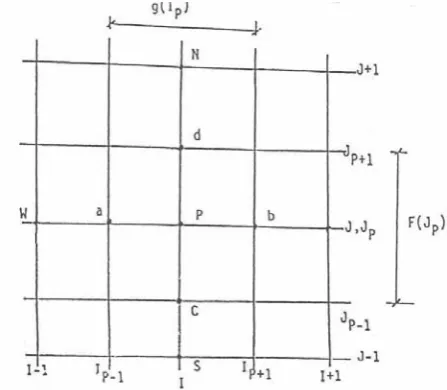
Finite difference has been used to solve equations governing the flow field on the spillways of dam. In this method the central difference approximation expresses the values and the partial derivatives of each formulation in a control volume as in figure l.
Figure 1. Grid points with control volume + ⎥ ⎦ ⎤ ⎢ ⎣ ⎡ ξ ∂ ∂ + − + ξ ∂ ∂ ξ η ξ η u ) y y ( J R ) v y u y ( u e 2 2 1 ⎥ ⎦ ⎤ ⎢ ⎣ ⎡ η ∂ ∂ + − + − η ∂ ∂ η ξ η ξ u ) y y ( J R ) y u y ( u e 2 2 1
p
y
)
p
y
(
p
y
(
η ξ−
ξηη
∂
∂
+
ξ
∂
∂
−
=
(35)
η ξ
ξ η ξ η ξ η ∂
∂ + ⎥ ⎦ ⎤ ⎢ ⎣ ⎡ + ′ − ′ ∂ ∂ − ′ − ′ ′ ∂ ∂ p y v y u y R v y u y u J e ) ( 1 ) ( 0 ) ( 1 ) ( ⎥= ⎦ ⎤ ⎢ ⎣ ⎡ − ′ − ′ ∂ ∂ − ′ − ′
′ y u y v y p
R v y u y v J e ξ ξ η ξ η
η
⎥ ⎦ ⎤ ⎢ ⎣ ⎡ + ′ + ′ ∂ ∂ − ′ + ′ ′ ∂ ∂ p v v y u y R v y u y u J e ξ η ξ η ξξ
η
( )1 ) ( 0 ) ( 1 ) ( ⎥= ⎦ ⎤ ⎢ ⎣ ⎡ ′+ ′ + ∂ ∂ − ′ + ′ ′ ∂ ∂
+ y u y v y p
R v y u y v J e η η ξ η ξ η η ξξ ηη ξ
η y y y
y J u VL
- 101 - Vol. 18, No. 1, February 2005 International Journal of Engineering 10
International Journal of Engineering Vol. 18, No. 1, February 2005 -11 In order to linearize some parts of equation 43, we
can use the remaining Terms of the later equation in higher order to form the new equation in ξ
direction and Navier-Stocks in η direction. Therefore by using finite difference forms of
ξ
and y the velocity field u and v can be determined.After determination of pressure and velocity fields the pressure and velocity variations show the cavitation points where the pressure is negative as shown in figure 6.
The general form of Navier-Stockes equation 36 can be written in direction
ξ
as: ⎥ ⎦ ⎤ ⎢ ⎣ ⎡ ′ − ′ ξ ∂ ∂ − ′ − ′ ξ ∂ ∂ ξ η ξη (y u y v)
R v u Jy u Jy e 1 2 ⎥ ⎦ ⎤ ⎢ ⎣ ⎡ ′ − ′ η ∂ ∂ − ′ − ′ ′ η ∂ ∂
+ η ξ (yηu yξv) R v Jy u v Jy e 1
2 (42)
ξ
∂
∂
−
η
∂
∂
=
y
ξp
y
ηp
First by integration of equation 36 we can write:
∫ ∫
⎥ ⎦ ⎤ ⎢ ⎣ ⎡ ξ ∂ ′ ∂ − ′ − ξ ∂ ′ ∂ + ′ − ′ − ′ ξ ∂ ∂ ξ ξξ η ξη ξ η d c b a e ) v y v y u y u y ( R v u Jy uJy 2 1
∫ ∫
⎥ η ξ⎦ ⎤ ⎢ ⎣ ⎡ η ∂ ′ ∂ − ′ − η ∂ ′ ∂ + ′ − − ′ − ′ ′ η ∂ ∂ + η
ξ b η ξ ξξ η ξη ξ
a d c e d d ) v y v y u y u y ( R v Jy v u Jy d
d 2 1
∫ ∫
∫ ∫
ξ
η
ξ
∂
∂
−
ξ
η
η
∂
∂
=
b ξ ηa d c d c b
a
(
y
p
)
d
d
d
d
)
p
y
(
(43) The finite difference form of equation 43 can be written as:∫ ∫
⎥ ξ η⎦ ⎤ ⎢ ⎣ ⎡ ξ ∂ ′ ∂ − ′ − ξ ∂ ′ ∂ + ′ − ′ ′ − ′ η ∂ ∂ ξ ξξ η ξη ξ η d c b a e d d ) v y v y u y u y ( R v u Jy u Jy 1 ⎩ ⎨ ⎧ ⎢ ⎣ ⎡ ξ ∂ ′ ∂ − ′ − ξ ∂ ′ ∂ + ′ − ′ ′ − ′
= (GA) u (yy) ( u ) (ZG) v (yx) ( v ) R v u ) BT ( u _) AL
( b b b b b b b
e b b b b b 1 2
)
J
(
F
)
v
(
)
yx
(
v
)
ZG
(
)
u
(
)
yy
(
u
)
GA
(
R
v
u
)
BT
(
u
)
AL
(
a a a a a a a a pe a a a a a
⎥
⎦
⎤
⎢
⎣
⎡
ξ
∂
′
∂
−
′
−
ξ
∂
′
∂
+
′
+
′
′
+
′
−
21
(44) The central difference forms of equation can be written as:
- 101 - Vol. 18, No. 1, February 2005 International Journal of Engineering 12
[
g
(
I
)
g
(
I
)
]
v
v
v
v
)
I
(
g
)
I
(
g
v
v
v
v
)
v
(
p p W NE E NE p p W Nw E NE b 1 1 1 12
2
2
+ − + −+
′
−
′
−
′
+
′
=
+
′
+
′
−
′
+
′
=
ξ
∂
′
∂
(46)⎥
⎥
⎦
⎤
⎢
⎢
⎣
⎡
′
−
′
=
ξ
∂
′
∂
′
+
′
′
+
′
=
′
−)
I
(
F
u
u
)
u
(
,
)
u
u
(
u
u
u
p w p a w p w p a 2 22
2
(47)[
F
(
I
)
F
(
I
)
]
V
V
V
V
)
v
(
,
V
V
V
p p WW . NWW . p . N . a w . NE . a3
1
2
2
−
+
−
′
−
′
−
′
+
′
=
ξ
∂
′
∂
′
+
′
=
′
⎩ ⎨ ⎧ ′ + ′ − ′ + ′ ′ + ′ = − 2 2 2 2 w . P . p P p E p E . p p u u ) J , I ( AL ) u u ( u u ) J , I ( ALBy substituting the equations 45, 46 and 47 into equation 44 we can write the following equation:
By using equation 49 we can write the general form of equation as follow:
{
C
1(
u
′
E+
u
′
P)
−
C
2(
u
′
p+
u
′
w)
−
C
3(
u
′
E−
u
′
p)
+
C
4(
u
′
p−
u
′
w)
+
C
5}
International Journal of Engineering Vol. 18, No. 1, February 2005 -13
( )
[
F
JP
F
(
JP
)
]
V
V
V
V
)
v
(
.N .NWW .S .W c2
2
+
−
′
−
′
−
′
+
′
=
η
∂
′
∂
(54) Substituting equations 51 through 54 into equation 50 gives the following equation:
{
F
1(
u
′
N+
u
′
p)
−
F
2(
u
′
p+
u
′
S)
−
F
3(
u
′
N−
u
′
p)
+
F
4(
u
′
p−
u
′
S)
+
F
5}
The finite difference form of the last term of right hand side in equation 43 can be written as:
∫
∫
∫ ∫
ξ
η
ξ
−
ξ
η
η
∂
∂
η ξ
b
a
d
c b
a d
c
d
(
y
P
)
d
d
d
)
d
d
)(
P
y
(
{
[(
YX
)
dP
d−
(
YX
)
cP
c]
g
(
I
p 1)
−
[(
YY
)
bP
b−
(
YY
)
aP
a]
F
(
JP
)}
=
−]
P
)
J
,
I
(
YY
P
)
JP
,
I
(
YY
)[
JP
(
f
{
p w−
p p p=
−2 (55)]} 4
) , ( 4
) , ( )
( 1 1 1 . . . . 1 1 .p .w .s .sw
p p w
p NM N p p p
P P P P J I YX P P P P J I YX I
g ⎢ − + + +
⎣
⎡ + + +
+ − − + − −
- 101 - Vol. 18, No. 1, February 2005 International Journal of Engineering 14
By considering the variables T1, T2 and T3 the equation 55 can be written as:
T1Pw- T2Pp+T3
Therefore, overall finite difference form of Navier-Stockes equation in
ξ
direction can be written as: ) u u ( C ) u u ( C ) u u ( C ) u u (C1 ′E+ ′p − 2 ′p+ ′w − 3 ′E− ′p + 4 ′p− ′w
)
u
u
(
F
)
u
u
(
F
)
u
u
(
F
C
+
′
N+
′
p−
′
p+
′
s−
′
N−
′
p+
5 1 2 33 2 1 5
4
(
u
u
)
F
T
P
T
P
T
F
′
p−
′
s+
=
w−
p+
+
(56) We can use coefficients for the convergence. Similarly, the finite difference form of Navier-Strockes equation in
η
direction can be written as:3 2 1 5 4 3 2 1 5 4 3 2 1 K P K P K W ) V V ( W ) V V ( W ) V V ( W ) V V ( W Z ) V V ( Z ) V V ( Z ) V V ( Z ) V V ( Z s p s p p N s p p N w p p E w p p E + + − = + ′ − ′ + ′ − ′ − ′ + ′ − ′ + ′ + ′ − ′ + ′ − ′ − ′ + ′ − ′ + ′ (57) For finite difference form of pressure equation by using velocity in
ξ
and y directions and equation of continuity gives the following equation:0 1 1 1 1 1 1 = ′ − + ′ + ′ − + ′ × − + − + ) J , I ( v ) J , I ( J ) IP ( g ) J , I ( v ) I , I ( J ) IP ( g ) J , I ( u ) J , J ( J ) JP ( F ) J , I ( u ) J , I ( J ) JP ( F p p p p p p p (58) 0 1
1 2 3 4
1u′(I+ ,J)−E u′(I,J)+E v′(I,J+ )−E v′(J,J)=
E
(59) Then by using equation 56 and 57 the Velocity field u′ and v′can be calculated in I and J element. 6 5 4 3 2
1 O p O P O P O P O
O
pp× = ×Δ p+ Δ w+ Δ N + Δ s−
Δ
(60)
In fact equation 60 shows the subtraction of inflow and outflow in a control volume and O6 is a convergence index.
7. Boundary Conditions
Since the spillway bed can be considered as the lower flow line and water surface as the upper flow line, therefore the components of the flow velocity u and v are zero.
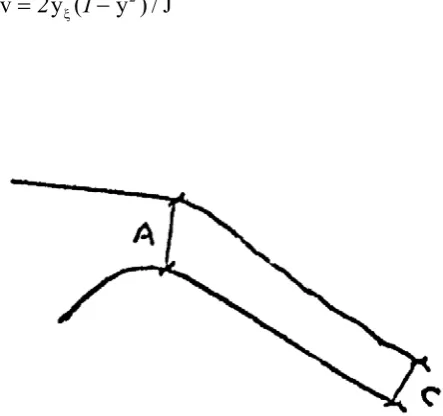
According to the figure.3 the boundary condition at section A can be written as:
J
/
)
y
(
y
v
J
/
)
y
(
y
u
2 21
2
1
2
−
=
−
=
ξ ηFigure 3. Boundary conditions
In which, u and v is far from section A where:
0
=
ξy
andy
η=
1
Therefore J=1 and for spillway bed u=0 and v=0
⎩ ⎨ ⎧ − = = ) y ( u v 2 1 2 0
And in water surface:
y
ξ=
0
and=
0
η
∂
∂
u
The velocity u in section c as shown in figure 3 can be corrected as follow:
At first section
=
∫
−
∫
2 1 2 1 1 1 x x y yin
u
dy
V
dx
q
At first section
ξ η ξ
η
−
=
International Journal of Engineering Vol. 18, No. 1, February 2005 -15 At first section
η ξ η
ξ
+
=
−
=
(
y
u
y
v
)
,
dx
y
d
v
1By substituting u1 and v1 in to qin , we can write:
∫
− η+∫
+ η= η η ξ ξ ξ η
1
0
1
0 2
2 u y y v)d (y u y y v)d
y ( qin
∫
+ η=∫
η= 1 η ξ 0
1
0 2
2
1 1,JP)u( ,Jp)d (
J d
) u y u y ( qin
Then, the flow in section before last is:
∫
= 1 0 J
qout ( in section before last)
d
η and velocity field inξ
direction: u (IN,JP)= u(IN-1,JP) + ( qin-qout)8. Model Application Results and Discussion
Two examples were considered for model application and comparing the solutions of mathematical model. In the first one the spillway of Marun dam which is an earth dam was analyzed. It is an ogee spillway with a height of 165 meters. The reservoir with 1290 million cubic meter capacity. Four radial gates 12 by 15 meter with 10000 return period flood and a capacity of 10800 m3/ sec. Employing different elements the results are depicted on graphs with the aid of water surface profile equation. The velocity and pressure field were determined and with investing the pressure, the cavitation was controlled.
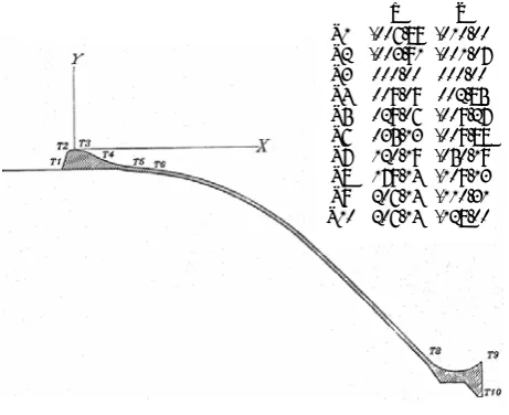
Figure 4 shows the x and y coordinates system of the Marun dam spillway near Behbehan city in Khozestan province of IRAN. Figures 5 and 6 show grid points and Mesh system of Marun spillway. The grid points near the gate and over the crest of spillway is smaller and different than other grid points in order to obtain better convergence.
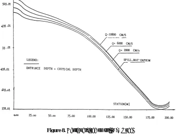
Figure 7 shows the water surface profile computed by the model. The results show that whit a flow of up to 4000 m3/sec the condition is good, but flows higher than this value, the water surface shows high uprising. The pressure at some points near gates was close to zero. Provisions are needed to prevent cavitation at these points. The results have been compared with spillway model and the
Figure 4. Coordinate System for SPILLWAY OF MARUN DAM
Figure 5. MESH NO. for marun spillway
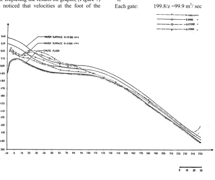
“USBR” laboratory findings (figure.8). It was observed that the results had relatively satisfactory stability and water surface profile was continuous. Figure 9 shows the pressure lines over the spillways for different flow rates. The maximum pressure occurs when flow is 10800 m3/se. Figure shows that at high water discharge vortex take place and secondary flows dominate near to lateral gates. As water discharge increases from 4000 m3/sec. The secondary flows begin to form and become maximum as discharge increases from 10800 m3/sec.
Y X
-010.00 -006.89 T1
-001.07 -003.91 T2
000.00 000.00 T3
002.85 009.09 T4
-009.27 029.06 T5
-009.88 035.13 T6
-050.19 120.19 T7
-109.13 179.14 T8
-110.31 206.14 T9
- 101 - Vol. 18, No. 1, February 2005 International Journal of Engineering 16
Figure 6. MESH NO. 4
In the second example “ABASPOUR” ogee spillway with a height of 200 m with 3 radial gates and maximum capacity of 15500 m3/sec was studied. Depicting the results on graphs, (Figure 9) it was noticed that velocities at the foot of the
chute was too high, nearly 50 m/sec. Negative pressures at some parts of the chute were observed. To compensate for this negative pressure, it is a necessary to use aeration ducts. Results were after ward compensate with those of “USBR”.
In this example for cavitation control the aeration ducts with 4000 m3/sec flow capacity and 15% air passage were used and the calculation for the determination of aeration systems are as follows:
15
0
.
q
q
C
w a
=
=
and design flow is 4000 m3/sec. The flow rate per unit width:sec
/
m
%)
.
(
q
w 372
5
8
3
40001
×
=
=
The aeration rate per unit width:
sec
/
m
.
/
q
a 38
10
100
15
72
×
=
=
Therefore the aeration in middle gate:
sec
/
m
.
.
.
q
a 38
199
5
18
8
10
×
=
=
Each gate: 199.8/z =99.9 m3/ sec
International Journal of Engineering Vol. 18, No. 1, February 2005 -17 And the aerator velocity:
va=70 m/sec
with the area of Aa=99.9/70=1.43 m2 The required air for aeration: Qa=qaL=10.8*18.5=199.8 m/sec
In each air channel and the total area needed: Aa=199.8/70=2.85 m2
The air gradually diffuse into water at the points where the pressure is negative and cavitation takes place and then the cavitation will be controlled.
Figure 8. Depth obtained on spillway model
Figure 9. Pressure and water surface profiles for different flow rates
- 101 - Vol. 18, No. 1, February 2005 International Journal of Engineering 18
9. References
1. Brown, F.R.F., ASCE (task force), “Cavitation in hydraulic structures”, 1963.
2. Beauchemin, P. and C. March, “An efficient finite element in compressible navier-Stokes, Salver that approximate non-linear terms with finite differences”, finite element in Analysis and Design, 10(1991), 235-242.
3. Carnuhan, B., “Applied numerical methods”, John wiley, New York, 1964.
4. Diersh, Hans-Joerg, A. Schirmer and K. Busch, “Analysis of flows with initially unknown discharge”, ASCE, Jr. of Hyd, Div. (Hy3), 1977, March.
5. Knapp, R.T., Daily J.W. and Hamitt. F.G. “Cavitation” MC-Graw-Hill book, Co. 1910. 6. Hamilton, W.S., “preventing cavitation damage
to hydraulic structures”, water power and dam cons, Nov. 1983.
7. Haris, P.J., “A numerical model for determination of motion of a bubble close to a fixed rigid structure in a fluid”, International Journal for numerical methods in Engineering, Vol. 33, 1813-1882 (1992).
8. Maynord.S.T. “General spillway investigation” Tech.Rep.HL-85-1, U.S. Army Engineer water ways Experiment station. Vicksburg, Miss (1985)
9. U.S. Army corp of Engineers (USACE) “Hydraulic design of spillways” Em 1110-21603 (1990).
10. Guo, Y. Wen.X., WU.C. and fang .D. Numerical modeling of spillway flow with free drop and initially unknown discharg” .Hydr, Res. Delft, the Netherlands, 36(5), 785-801 (1998).
11. Burgisser, M.F., and Rutschamann, P. Numerical solution of viscouse 2Dv free surface flows; flow over spillway crests. Proc., 28 th IAHR congr. Technical universal Graz, Graz. Austria (1999).
12. Olsen, N.R., and Kjellesvig, H.M. “Three dimensional numerical flow modeling for estimation of spillway capacity”, J.Hydr.Res.r, Dlft, the Netherlands, 36 (5) , 775-784 (1998). 13. Bruce M. Suvage, and Johnson, M.C., “flow
over ogee spillway: physical and Numerical Model case study” J. Hydr.Eng. ASCE Vol. 127. NO. 8, August 2001.
14. Ramaswamy, B. and T.C. Jue, “A segregated finite element formulation of Navier- Stocks equations under laminar conditions”, Finite elements in analysis and Design, (1991) 257-270.
15. Pinto, Nl. Des. S.H. Neidert and J.J. ota, “Aeration at high velocity flows”, water power and dam construction, March 1982.
16. Rutchmann, P. and Will, H. hager, “Air entrainment by spillway aerators”, ASCE Journal of the Hydraulic Division, Vol.116, 1990.
17. Thompson and Mastin, “Numerical grid generation foundation and Applications”, North Holland, 1985.
18. Thompson, J.F., 1982, “General curvilinear coordinate system, numerical grid generation”, (J.F. tampson Ed.).
Notations
The following symbols are used in this paper
Symbols a
b c d p T dξ
dη
d∀
du
V
F(JP) g(IP) Ire
V U U’ V’ Q
μ
Defined point over control “
“ “ “
Jacobian = δ2η + δ2η
derivative ξ
derivative η
control volume derivative u
mean velocity over dam spillways distance between two η
distance between two ξ
Reynolds number
velocity component at axis y velocity component at axis x velocity component at axis ξ
velocity component at axis η
discharge