Application of Fuzzy and ABC Algorithm for DG Placement
for Minimum Loss in Radial Distribution System
M. Padma Lalitha*, V.C. Veera Reddy** and N. Sivarami Reddy***
Abstract: Distributed Generation (DG) is a promising solution to many power system problems such as voltage regulation, power loss, etc. This paper presents a new methodology using Fuzzy and Artificial Bee Colony algorithm (ABC) for the placement of Distributed Generators (DG) in the radial distribution systems to reduce the real power losses and to improve the voltage profile. A two-stage methodology is used for the optimal DG placement. In the first stage, Fuzzy is used to find the optimal DG locations and in the second stage, ABC algorithm is used to find the size of the DGs corresponding to maximum loss reduction. The ABC algorithm is a new population based meta heuristic approach inspired by intelligent foraging behavior of honeybee swarm. The advantage of ABC algorithm is that it does not require external parameters such as cross over rate and mutation rate as in case of genetic algorithm and differential evolution and it is hard to determine these parameters in prior. The proposed method is tested on standard IEEE 33 bus test system and the results are presented and compared with different approaches available in the literature. The proposed method has outperformed the other methods in terms of the quality of solution and computational efficiency.
Keywords:ABC Algorithm, DG placement, Loss reduction, Meta Heuristic Methods, Radial Distribution System.
1 Introduction1
Distributed or dispersed generation (DG) or embedded generation (EG) is small-scale power generation that is usually connected to or embedded in the distribution system. The term DG also implies the use of any modular technology that is sited throughout a utility’s service area (interconnected to the distribution or sub-transmission system) to lower the cost of service [1]. The benefits of DG are numerous [2, 3] and the reasons for implementing DGs are an energy efficiency or rational use of energy, deregulation or competition policy, diversification of energy sources, availability of modular generating plant, ease of finding sites for smaller generators, shorter construction times and lower capital costs of smaller plants and proximity of the generation plant to heavy loads, which reduces transmission costs. Also it is accepted by many countries that the reduction in gaseous emissions
Iranian Journal of Electrical & Electronic Engineering, 2010. Paper first received 4 Apr. 2010 and in revised form 2 Oct. 2010. * The Author is with the Department of EEE, AITS, Rajampet, A.P. E-mail: [email protected]
** The Author is with the Department of EEE, S.V.U.C.E, S.V. University,Tirupathi, A.P.
E-mail: [email protected]
*** The Author is with the Department of ME, AITS, Rajampet, A.P. E-mail: [email protected].
(mainly CO2) offered by DGs is major legal driver for
DG implementation [4].
The distribution planning problem is to identify a combination of expansion projects that satisfy load growth constraints without violating any system constraints such as equipment overloading [5]. Distribution network planning is to identify the least cost network investment that satisfies load growth requirements without violating any system and operational constraints. Due to their high efficiency, small size, low investment cost, modularity and ability to exploit renewable energy sources, are increasingly becoming an attractive alternative to network reinforcement and expansion. Numerous studies used different approaches to evaluate the benefits from DGs to a network in the form of loss reduction, loading level reduction [6-8].
Naresh Acharya et al suggested a heuristic method in [9] to select appropriate location and to calculate DG size for minimum real power losses. Though the method is effective in selecting location, it requires more computational efforts. The optimal value of DG for minimum system losses is calculated at each bus. Placing the calculated DG size for the buses one by one, corresponding system losses are calculated and compared to decide the appropriate location. More over the heuristic search requires exhaustive search for all
possible locations which may not be applicable to more than one DG. This method is used to calculate DG size based on approximate loss formula may lead to an inappropriate solution.
In the literature, genetic algorithm and PSO have been applied to DG placement [10-13].In all these works both sizing and location of DGs are determined by these methods. This paper presents a new methodology using ABC algorithm [14-17] for the placement of DG in the radial distribution systems. The ABC algorithm is a new population based meta heuristic approach inspired by intelligent foraging behavior of honeybee swarm. The advantage of ABC algorithm is that it does not require external parameters such as cross over rate and mutation rate as in case of genetic algorithm and differential evolution and it is hard to determine these parameters in prior. The other advantage is that the global search ability in the algorithm is implemented by introducing neighborhood source production mechanism which is a similar to mutation process. The advantage of ABC algorithm is because of its simplicity it takes less computation time than PSO method.
In this paper, the optimal locations of distributed generators are identified based on the Fuzzy method [18] and ABC optimization technique which takes the number and location of DGs as input has been developed to determine the optimal size(s) of DG to minimize real power losses in distribution systems. The advantages of relieving ABC method from determination of locations of DGs are improved convergence characteristics and less computation time. Voltage and thermal constraints are considered. The effectiveness of the proposed algorithm was validated using 33-Bus Distribution System [19]. To test the effectiveness of proposed method, results are compared with different approaches available in the literature. The proposed method has outperformed the other methods in terms of the quality of solution and computational efficiency.
2 Theoretical Background
The total I
2
R loss (PL) in a distribution system
having n number of branches is given by:
n 2
Lt i
i 1
P I Ri
=
=
∑
(1)here Ii is the magnitude of the branch current and Ri is
the resistance of the ithbranch respectively. The branch current can be obtained from the load flow solution. The branch current has two components, active component (Ia) and reactive component (Ir). The loss associated
with the active and reactive components of branch currents can be written as:
n 2 La ai
i 1
P I Ri
=
=
∑
(2)n 2 Lr ri
i 1
P I Ri
=
=
∑
(3)Note that for a given configuration of a single-source radial network, the loss PLaassociated with the
active component of branch currents cannot be minimized because all active power must be supplied by the source at the root bus. However by placing DGs, the active component of branch currents are compensated and losses due to active component of branch current is reduced. This paper presents a method that minimizes the loss due to the active component of the branch current by optimally placing the DGs and thereby reduces the total loss in the distribution system. A two stage methodology is applied here. In the first stage optimum location of the DGs are determined by using fuzzy approach and in the second stage an analytical method is used to determine sizes of the DGs for maximum real loss reduction.
3 Identification of Optimal DG Locations using Fuzzy Approach
This paper presents a fuzzy approach to determine suitable locations for DG placement. Two objectives are considered while designing a fuzzy logic for identifying the optimal DG locations. The two objectives are: (i) to minimize the real power loss and (ii) to maintain the voltage within the permissible limits. Voltages and power loss indices of distribution system nodes are modeled by fuzzy membership functions. A fuzzy inference system (FIS) containing a set of rules is then used to determine the DG placement suitability of each node in the distribution system. DG can be placed on the nodes with the highest suitability.
For the DG placement problem, approximate reasoning is employed in the following manner: when losses and voltage levels of a distribution system are studied, an experienced planning engineer can choose locations for DG installations, which are probably highly suitable. For example, it is intuitive that a section in a distribution system with high losses and low voltage is highly ideal for placement of DG. Whereas a low loss section with good voltage is not ideal for DG placement. A set of fuzzy rules has been used to determine suitable DG locations in a distribution system.
In the first step, load flow solution for the original system is required to obtain the real and reactive power losses. Again, load flow solutions are required to obtain the power loss reduction by compensating the total active load at every node of the distribution system. The loss reductions are then, linearly normalized into a [0, 1] range with the largest loss reduction having a value of 1 and the smallest one having a value of 0. Power Loss Index [15] value for ith node can be obtained using equation 4.
(Lossreduction(i) Lossreduction(min))
PLI(i)
(Lossreduction(max) Lossreduction(min))
− =
− (4) These power loss reduction indices along with the p.u. nodal voltages are the inputs to the Fuzzy Inference
System (FIS), which determines the nodes that are more suitable for DG installation.
3.1 Implementation of Fuzzy Method
In this paper, two input and one output variables are selected. Input variable-1 is power loss index (PLI) and Input variable-2 is the per unit nodal voltage (V). Output variable is DG suitability index (DSI). Power Loss Index range varies from 0 to 1, P.U. nodal voltage range varies from 0.9 to 1.1 and DG suitability index range varies from 0 to 1.
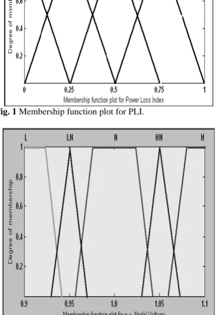
Five membership functions are selected for PLI. They are L, LM, M, HM and H. All the five membership functions are triangular as shown in Fig. 1. Five membership functions are selected for Voltage. They are L, LN, N, HN and H. These membership functions are trapezoidal and triangular as shown in Fig. 2. Five membership functions are selected for DSI. They are L, LM, M, HM and H. These five membership functions are also triangular as shown in Fig. 3.
Fig. 1 Membership function plot for PLI.
Fig. 2 Membership function plot for voltage.
Fig. 3 Membership function plot for DSI.
For the DG allocation problem, rules are defined to determine the suitability of a node for capacitor installation. Such rules are expressed in the following form: IF premise (antecedent), THEN conclusion (consequent).
For determining the suitability of DG placement at a particular node, a set of multiple-antecedent fuzzy rules has been established. The inputs to the rules are the voltage and power loss indices and the output is the suitability of DG placement. The rules are summarized in the fuzzy decision matrix in Table 1. In the present work 25 rules are constructed.
Table 1 Fuzzy Decision Matrix.
AND
Voltage
LL LN NN HN HH
DSI
L LM LM L L L
LM M LM LM L L
M HM M LM L L
HM HM HM M LM L
H H HM M LM L
4 Identification of Optimal DG Sizes by ABC Algorithm
4.1 Introduction to ABC Algorithm
In the ABC algorithm, the colony of artificial bees contains three groups of bees: employed bees, onlookers and scouts. A bee waiting on the dance area for making decision to choose a food source is called an onlooker and a bee going to the food source visited by it previously is named an employed bee. A bee carrying out random search is called a scout. In the ABC algorithm, first half of the colony consists of employed artificial bees and the second half constitutes the onlookers. For every food source, there is only one employed bee. In other words, the number of employed bees is equal to the number of food sources around the hive. The employed bee whose food source is exhausted by the employed and onlooker bees becomes a scout. In
the ABC algorithm, each cycle of the search consists of three steps: sending the employed bees onto the food sources and then measuring their nectar amounts; selecting of the food sources by the onlookers after sharing the information of employed bees and
determining the nectar amount of the foods; determining the scout bees and then sending them onto possible food sources. At the initialization stage, a set of food source positions are randomly selected by the bees and their nectar amounts are determined. Then, these bees come in to the hive and share the nectar
information of the sources with the bees waiting on the dance area within the hive. At the second stage, after sharing the information, every employed bee goes to the food source area visited by her at the previous cycle since that food source exists in her memory, and then chooses a new food source by means of visual information in the neighborhood of the present one. At the third stage, an onlooker prefers a food source area depending on the nectar information distributed by the employed bees on the dance area. As the nectar amount of a food source increases, the probability with which that food source is chosen by an onlooker increases, too. Hence, the dance of employed bees carrying higher nectar recruits the onlookers for the food source areas with higher nectar amount. After arriving at the selected area, she chooses a new food source in the neighborhood of the one in the memory depending on visual information. Visual information is based on the comparison of food source positions. When the nectar of a food source is abandoned by the bees, a new food source is randomly determined by a scout bee and replaced with the abandoned one. In our model, at each cycle at most one scout goes outside for searching a new food source and the number of employed and onlooker bees were equal. The probability Pi of selecting a food source i is determined using the following expression:
N i i S
n n 1
fit P
fit
= =
∑
(5)where fitiis the fitness of the solution represented by the
food source i and SN is the total number of food sources. Clearly, with this scheme good food sources will get more onlookers than the bad ones. After all onlookers have selected their food sources, each of them determines a food source in the neighborhood of his chosen food source and computes its fitness. The best food source among all the neighboring food sources determined by the onlookers associated with a particular food source i and food source i itself, will be the new location of the food source i. If a solution represented by a particular food source does not improve for a predetermined number of iterations then that food source is abandoned by its associated employed bee and it becomes a scout, i.e., it will search for a new food source randomly. This tantamount to assigning a randomly generated food source (solution) to this scout and changing its status again from scout to employed. After the new location of each food source is determined, another iteration of ABC algorithm begins. The whole process is repeated again and again till the termination condition is satisfied. The food source in the
neighborhood of a particular food source is determined by altering the value of one randomly chosen solution parameter and keeping other parameters unchanged. This is done by adding to the current value of the chosen parameter the product of a uniform variate in [-1, 1] and the difference in values of this parameter for this food source and some other randomly chosen food source. Formally, suppose each solution consists of d parameters and let Xi = (Xi1, Xi2, Xi3, …, Xid) be a
solution with parameter values Xi1, Xi2, Xi3, …, Xid. In
order to determine a solution vi in the neighborhood of
Xi, a solution parameter j and other solution Xk=(Xk1,
Xk2, Xk3, …, Xkd) are selected randomly. Except for the
values of the selected parameter j, all other parameter values of vi are same as Xi, i.e., vi=(Xi1, Xi2 … Xi(j-1),
Xij, Xi(j+1), … Xid). The value vi of the selected
parameter j in vi is determined using the following
formula:
ij ij ij kj
v =x +u(x −x ) (6)
where uis an uniform variate in [-1, 1]. If the resulting value falls outside the acceptable range for parameter j, it is set to the corresponding extreme value in that range.
4.2 Problem Formulation
n 2
M in P I R
Lt i 1 i i
⎧ ⎫
⎪ = ∑ ⎪
⎨ ⎬
⎪ = ⎪
⎩ ⎭ (7)
Subject to voltage and current constraints:
V V V
i m in ≤ i ≤ i m ax
(8)
I I
ij ≤ ij m ax
(9)
where Ii is the current flowing through the ith branch
which is dependent on the locations and sizes of the DGs. Locations determined by fuzzy method are given as input. So the objective function is now only dependent on the sizes of the DGs at these locations.
Ri is the resistance of the ith branch. Vimax and Vimin
are the upper and lower limits on ith bus voltage. Iijmax is
the maximum loading on branch ij. The important operational constraints on the system are addressed by equations 8 and 9.
4.3 Assigned Values for Various Parameters of ABC Method
The assigned values for various parameters of ABC method are as follows.
• Number of Total Bees = 40 • Number of Employed bees = 20 • Number of Onlooker bees = 20 • Number of Scout Bee = 1
• Stopping Criterion --- (Maximum Fitness – Average Fitness) < 10-12
4.4 Algorithm to Find the DG Sizes at Desired Locations using ABC Algorithm
The proposed ABC algorithm for finding sizes of DGs at selected locations to minimize the real power loss is summarized as follows:
1. Read the input data; Initialize MNC (Maximum Iteration Count) and base case as the best solution.
2. Construct initial Bee population (solution) xijas
each bee is formed by the sizes of DG units and the number of employed bees are equal to onlooker bees.
3. Evaluate fitness value for each employed bee by using the following the formula
1 fitness
1 PowerLoss
=
+ (10) 4. Initialize iteration = 1.
5. Generate new population (solution) vij in the
neighborhood of xij for employed bees using
equation (6) and evaluate them.
6. Apply the greedy selection process between xi
and vi.
7. Calculate the probability values Pi for the solutions xi by means of their fitness values using the equation (5).
8. Produce the new populations vi for the onlookers from the populations x, selected depending on Pi by applying roulette wheel selection process, and evaluate them.
9. Apply the greedy selection process for the onlookers between xiand vi.
10.Determine the abandoned solution, if exists, and replace it with a new randomly produced solution xi for the scout bees using the following equation
ij j j j
x =min +rand(0,1) * (max−min ) (11)
11.Memorize the best solution achieved so far. If the difference between two successive values is less than specified value, go to step 14.
12.Increase the iteration number by one.
13.If iterations are less than MIC, go to step 5, otherwise go to step 14.
14.Stop.
5 Results and Discussion
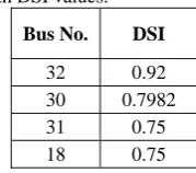
First load flow is conducted for IEEE 33 bus test system [7]. The power loss due to active component of current is 136.9836 kW and power loss due to reactive component of the current is 66.9252 kW. Optimal DG locations are identified based on the DSI values. For this 33 bus system, four optimal locations are identified. The candidate locations with their DSI values are given in Table 2.
Table 2 Buses with DSI values.
Bus No. DSI
32 0.92 30 0.7982 31 0.75 18 0.75
The locations determined by Fuzzy method for DG placement are 32,30,31,18. With these locations, sizes of DGs are determined by using ABC Algorithm described in section 4. The sizes of DGs are dependent on the number of DG locations. Generally it is not possible to install many DGs in a given radial system. Here 4 cases are considered. In case I only one DG installation is assumed. In case II two DGs, in case III three DGS and in the last case four DGs are assumed to be installed. DG sizes in the four optimal locations, total real power losses before and after DG installation for four cases are given in Table 3.
Table 3 Results of IEEE 33 bus system.
Case DG
locations
DG sizes (MW)
Total Size (MW)
Losses before DG installation
(kW)
Loss after DG installation
(kW)
Saving (kW) Saving/DG
size
I 32 1.2931 1.2931 203.9088 127.0919 76.817 59.405
II 32 0.3836 1.5342 203.9088 117.3946 86.5142 56.39
30 1.1506
III
32 0.2701
1.5342 203.9088 117.3558 86.553 56.41 30 1.1138
31 0.1503
IV
32 0.2701
1.8423 203.9088 90.292 113.6166 61.67
30 0.8233 31 0.1503 18 0.5986
The last column in Table 3 represents the saving in kW for 1 MW DG installation. The case with greater ratio is desirable. As the number of DGs installed is
increasing the saving is also increasing. In case4 maximum saving is achieved but the number of DGs is four. Though the ratio of saving to DG size is maximum
of all cases which represent optimum solution but the number of DGs involved is four so it is not economical by considering the cost of installation of 4 DGs. But in view of reliability, quality and future expansion of the system it is the best solution.
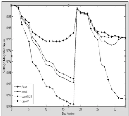
Table 4 shows the minimum voltage and % improvement in minimum voltage compared to base case for all the four cases. In all the cases voltage profile is improved and the improvement is significant. The voltage profile for all cases is shown in Fig. 4.
Table 4 Voltage improvement with DG placement.
Case No. Bus No. Min Voltage % Change
Base Case 18 0.9118
Case1 18 0.9314 2.149 Case2 18 0.9349 2.533 Case3 18 0.9349 2.533 Case4 14 0.9679 6.153
Table 5 shows % improvements in power loss due to active component of branch current, reactive component of branch current and total active power loss of the system in the four cases considered. The loss due to active component of branch current is reduced by more than 68% in least and nearly 96% at best. Though the aim is reducing the PLa loss, the PLr loss is also reducing
due to improvement in voltage profile. From Table 5 it is observed that the total real power loss is reduced by 48.5% in case 1 and 67% in case 4.
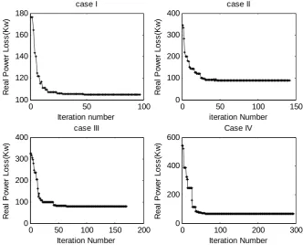
The convergence characteristics of the solution of ABC algorithm for all the four cases are shown in Fig. 5.
Table 6 shows the minimum, average and maximum values of total real power loss from 100 trials of ABC algorithm. The average number of iterations and average CPU time are also shown.
5.1 Comparison Performance
To demonstrate the validity of the proposed method the results of proposed method are compared with an existing PSO method [20]. The comparison is shown in Table 7.
From the above tables it is clear that the proposed method is producing the results that match with those of
existing method. The two methods are tested on four IEEE standard test systems viz. 15 Bus, 34 Bus, 69 Bus and 85 Bus system. The results of these two methods for all the test system are identical. To demonstrate the supremacy of the proposed method the convergence characteristics are compared with that of PSO algorithm as shown in Table 8. Though the number of iterations is more for ABC algorithm it takes less computation time because of its simplicity when compared to PSO method.
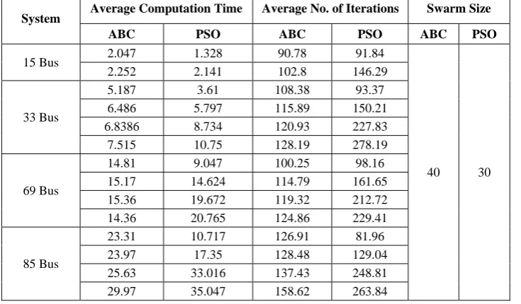
The convergence characteristics of the proposed ABC method and PSO methods for remaining test system are given in Table 9.
From the above table it is clear that the time taken for one iteration is very small for ABC compared to PSO method. For small systems the convergence characteristics of ABC method are better than PSO method. For large systems for less number of DG units the convergence characteristics of ABC Method are better than PSO method. When four DG units are to be placed in the system then PSO method is taking less time than ABC method. But generally it is very rare case.
Fig. 4 Voltage profile with and without DG placement for all
Cases.
Table 5 Loss reduction by DG placement.
Case No. PLa(kW) % Saving PLr(kW) % Saving PLt(kW) % Saving
Base case 136.9836 ---- 66.9252 ---- 203.9088 ----
Case1 62.7085 54.22 64.3834 3.7979 127.0919 37.45
Case2 53.6323 60.847 63.7623 4.726 117.3946 42.43
Case3 53.5957 60.874 63.7601 4.729 117.3558 42.45
Case4 27.7143 79.768 62.5779 6.4957 90.292 55.72
Table 6 Performance of ABC algorithm for IEEE 33 Bus System.
Total real power loss (kW) Case I Case II Case III Case IV
Min 105.023 89.9619 79.2515 66.5892
Average 105.023 89.9619 79.2515 66.5892
Max 105.023 89.9619 79.2515 66.5892
Bee swarm Size 40 40 40 40
Avg. No. of iterations 93.45 118.73 196.75 256.34
Average Time (Sec.) 3.344 4.89 7.89 10.14
Table 7 Comparison of results of IEEE 33-bus system by proposed method and other existing method.
Case Bus
Locations
Sizes (MW) Total Size (MW) Saving (kW)
ABC PSO ABC PSO ABC PSO
1 32 1.2931 1.2931 1.1883 1.1883 76.3619 76.3619
2 32 0.3836 0.3836
1.416 1.416 86.0246 86.0246
30 1.1506 1.1506
3
32 0.2701 0.2701
1.416 1.416 86.0628 86.0628
30 1.1138 1.1138
31 0.1503 0.1503
4
32 0.27006 0.2700
6
1.86176 1.86176 113.4294 113.4294
30 0.8432 0.8432
31 0.1503 0.1503
18 0.5982 0.5982
Table 8 Comparison of results of ABC and PSO algorithms.
Case I Case II Case III Case IV
ABC PSO ABC PSO ABC PSO ABC PSO
Swarm Size 40 30 40 30 40 30 40 30
Avg. No. of
iterations 93.45 98.26 118.73 127.06 196.75 145.81 256.54 171.69
Avg. time(sec.) 3.344 5.234 4.89 6.39 7.89 8.688 10.14 10.78
Table 9 Comparison of convergence characteristics of ABC and PSO algorithms.
System Average Computation Time Average No. of Iterations Swarm Size
ABC PSO ABC PSO ABC PSO
15 Bus 2.047 1.328 90.78 91.84
40 30
2.252 2.141 102.8 146.29
33 Bus
5.187 3.61 108.38 93.37
6.486 5.797 115.89 150.21
6.8386 8.734 120.93 227.83
7.515 10.75 128.19 278.19
69 Bus
14.81 9.047 100.25 98.16
15.17 14.624 114.79 161.65
15.36 19.672 119.32 212.72
14.36 20.765 124.86 229.41
85 Bus
23.31 10.717 126.91 81.96
23.97 17.35 128.48 129.04
25.63 33.016 137.43 248.81
29.97 35.047 158.62 263.84
0 50 100 100
120 140 160 180
Iteration number
Re
a
l P
o
we
r L
o
s
s
(K
w)
case I
0 50 100 150
0 100 200 300 400
iteration Number
Re
a
l P
o
we
r L
o
s
s
(K
w)
case II
0 50 100 150 200
0 100 200 300 400
Iteration Number
R
e
al
P
o
w
e
r Los
s
(K
w
)
case III
0 100 200 300
0 200 400 600
Iteration Number
R
e
al
P
o
w
e
r Los
s
(K
w
)
Case IV
Fig. 5 Convergence characteristic of ABC algorithm for 33 bus test system.
6 Conclusion
In this paper, a two-stage methodology of finding the optimal locations and sizes of DGs for maximum loss reduction of radial distribution systems is presented. Fuzzy method is proposed to find the optimal DG locations and a ABC algorithm is proposed to find the optimal DG sizes. Voltage and line loading constraints are included in the algorithm.
The validity of the proposed method is proved from the comparison of the results of the proposed method with other existing methods. The results proved that the ABC algorithm is simple in nature than GA and PSO so it takes less computation time. By installing DGs at all the potential locations, the total power loss of the system has been reduced drastically and the voltage profile of the system is also improved. Inclusion of the real time constrains such as time varying loads and different types of DG units and discrete DG unit sizes into the proposed algorithm is the future scope of this work.
References
[1] Celli G. and Pilo F., “Optimal distributed generation allocation in MV distribution networks,” 22nd IEEE Power Engineering Society International Conference, pp. 81-86, May 2001.
[2] Daly P.A., Morrison J., “Understanding the potential benefits of distributed generation on power delivery systems,” Rural Electri Power Conference, pp. A211-A213, April/May 2001.
[3] Chiradeja P., Ramakumar R., “An approach to quantify the technical benefits of distributed generation,” IEEE Trans Energy Conversion, Vol. 19, No. 4, pp. 764-773, 2004.
[4] “Kyoto Protocol to the United Nations Framework Convention on climate change,” Available at: http://unfccc.int/resource/docs/ convkp/kpeng.htm1.
[5] Brown R.E., Pan J., Feng X. and Koutlev K., “Siting distributed generation to defer T&D expansion,” Proc. IEE. Gen, Trans and Dist., Vol. 12, No. 3, pp. 1151-1159, 1997.
[6] Diaz-Dorado E., Cidras J., Miguez E., “Application of evolutionary algorithms for the planning of urban distribution networks of medium voltage,” IEEE Trans. Power Systems, Vol. 17, No. 3, pp. 879-884, Aug. 2002.
[7] Mardaneh M., Gharehpetian G. B., “Siting and sizing of DG units using GA and OPF based technique,” TENCON. IEEE Region 10 Conference, Vol. 3, pp. 331-334, Nov. 2004. [8] Berizzi S. A. and Buonanno S., “Distributed
generation planning using genetic algorithms,” Electric Power Engineering, Power Tech. Budapest 99, Int. Conference, pp. 257, 1999. [9] Acharya N., Mahat P. and Mithulanathan N., “An
analytical approach for DG allocation in primary distribution network”, Electric Power and Energy Systems, Vol. 28, No. 6, pp. 669-678, 2006. [10] Celli G., Ghaini E., Mocci S. and Pilo F., “A
multi objective evolutionary algorithm for the
sizing and sitting of distributed generation,” IEEE Transactions on Power Systems, Vol. 20, No. 2, pp. 750-757, May 2005.
[11] Carpinelli G., Celli G., Mocci S. and Pilo F., “Optimization of embedded sizing and sitting by using a double trade-off method,” IEE proceeding on Generation, Transmission and Distribution, Vol. 152, No. 4, pp. 503-513, 2005.
[12] Borges C. L. T. and Falcao D. M., “Optimal distributed generation allocation for reliability, losses and voltage improvement,” International Journal of Power and Energy Systems, Vol. 28, No. 6, pp. 413-420, July 2006.
[13] Krueasuk W. and Ongsakul W., “Optimal Placement of Distributed Generation Using Particle Swarm Optimization,” M. Tech. Thesis, AIT, Thailand, 2006.
[14] Karaboga D., “An idea based on honey bee swarm for numerical optimization,” Technical Report TR06, Computer Engineering Department, Erciyes University, Turkey, 2005.
[15] Basturk B. and Karaboga D., “An artificial bee colony (ABC) algorithm for numeric function optimization,” IEEE Swarm Intelligence Symposium 2006, Indianapolis, Indiana, USA, May 2006.
[16] Karaboga D. and Basturk B., “A powerful and efficient algorithm for numerical function optimization: artificial bee colony (ABC) algorithm,” Journal of Global Optimization, Vol. 39, No. 3, pp. 459-471, 2007.
[17] Karaboga D. and Basturk B., “On the performance of artificial bee colony (ABC) algorithm,” Applied Soft Computing, Vol. 8, No. 1, pp. 687-697, 2008.
[18] Padma Lalitha M., Veera Reddy V. C. and Usha N.,“DG Placement Using Fuzzy For Maximum Loss Reduction In Radial Distribution System,” International Journal of Computer Applications in Engineering, Technology and Sciences, Vol. 2, No. 1, pp. 50-55, Oct./Mar. 2010.
[19] Brara M. E. and Wu F. F., “Networ reconfiguration in distribution system for loss reduction and load balancing”, IEEE Transactions on Power Delivery, Vol. 4, No. 2, pp. 1401-1407, Apr. 1989.
[20] Padma Lalitha M., Veera Reddy V. C., Usha V. and Sivarami Reddy N.,” Application Of Fuzzy And PSO For DG Placement For Minimum Loss In Radial Distribution system,” ARPN Journal of Engineering and Applied Sciences, Vol. 5, No. 4, April 2010.
M. Padma Lalitha is pursuing Ph.D
and is a graduate from JNTU, Anathapur in Electrical & Electronics Engineering in the year 1994. Obtained Post graduate degree in PSOC from S.V.U, Tirupathi in the year 2002. Having 14 years of experience in teaching in graduate and post graduate level. Has 10 international journal publications and 10 international and national conferences to her credit. Presently working as Professor and HOD of EEE department in AITS, Rajampet. Areas of interest include radial distribution systems, artificial intelligence in power systems, ANN.
V. C. Veera Reddy presently working
as a professor in EEE department of S.V.U. College of Engineering, Tirupathi. He awarded Ph.D for his work “Modeling & Control of Load frequency using New Optimal Control strategy” from S.V.U. in the year 1999.Have 28 years of experience in teaching and worked in various levels. Guided a number of research scholars. Attended a number of national & international conferences. Areas of interest include Distribution systems, Genetic Algorithms, Fuzzi Systems, ANN.
N. Sivarami Reddy is pursuing Ph.D
and is a graduate from SRKREC, Bimavaram in Mechanical Engineering in the year 1989. Obtained Post graduate degree in Advanced Manufacturing Systems from NIT, Suratkal in the year 1992. Having 18 years of experience in teaching in graduate and post graduate level. Presently working as Professor and HOD of ME department in AITS, Rajampet. Areas of interest include Flexible Manufacturing systems, Soft computing techniques in FMS.