A SIMPLE TRANSFORMATION METHOD IN
SKEWNESS REDUCTION
B. Abbasi
Department of Mathematical and Geospatial Sciences, RMIT University Victoria, Australia
S.T. Akhavan Niaki* and S.E. Seyedan
Department of Industrial Engineering, Sharif University of Technology P.O. Box 11155-9414, Tehran, Iran
[email protected] - [email protected]
*Corresponding Author
(Received: May 16, 2009 – Accepted in Revised Form: June 21, 2011)
Abstract Statistical analysis of non-normal data is usually more complicated than that for normal distribution. In this paper, a simple root/power transformation technique developed by Niaki, et al [1] is extended to transform right and left skewed distributions to nearly normal. The value of the root/power is explored such that the skewness of the transformed data becomes almost zero with an acceptable error. The proposed method is then compared to the well-known and complicated Box, et al [2] transformation method for different left and right skewed distributions using Monte Carlo simulation. While the proposed procedure is easy to understand and to implement, the results of the simulation study show that it works as good as the Box-Cox method.
Keywords Root/Power Transformation, Box-Cox Transformation, Non-Normal Data Analysis
هﺪﯿﮑﭼ
ﻻﻮﻤﻌﻣ لﺎﻣﺮﻧ ﺮﯿﻏ يﺎﻫ هداديرﺎﻣآ ﻞﯿﻠﺤﺗ يﺎﻬﺷور "
لﺎﻣﺮﻧ يﺎﻫهداد ﻞﯿﻠﺤﺗيﺎﻬﺷور زاﺮﺗ هﺪﯿﭽﯿﭘ
ﺖﺳا
.
ﯽﮕﻟﻮﭼﭗﭼ وﺖﺳارﺖﻤﺳﻪﺑ ﻪﮐﯽﻟﺎﻤﺘﺣايﺎﻬﻌﯾزﻮﺗياﺮﺑ ﯽﻧاﻮﺗﻞﯾﺪﺒﺗ ةدﺎﺳشورﮏﯾ ،ﻪﻟﺎﻘﻣﻦﯾا رد ﺪﻨﮐ ﮏﯾدﺰﻧلﺎﻣﺮﻧﻊﯾزﻮﺗﻪﺑارﺎﻬﻧآﺎﺗدﻮﺷﯽﻣ هدادﻪﻌﺳﻮﺗ ﺪﻧراد
.
راﺪﻘﻣ يدﺪﻋشور زا هدﺎﻔﺘﺳاﺎﺑ ناﻮﺗيدﺪﻋ
ﻢﯿﻧشﺮﺑ ﻃ ﺎﺒﯾﺮﻘﺗارﺎﻫهدادرددﻮﺟﻮﻣﯽﮕﻟﻮﭼﻪﮐﺪﯾآﯽﻣﺖﺳدﻪﺑوﻮﺠﺘﺴﺟيرﻮ "
دﺮﺒﺑﻦﯿﺑزا
.
شوردﺮﮑﻠﻤﻋ
ﺲﮐﺎﺑ ةﺪﯿﭽﯿﭘ و فوﺮﻌﻣ شور دﺮﮑﻠﻤﻋ ﺎﺑ هﺎﮕﻧآ يدﺎﻬﻨﺸﯿﭘ
-ﺎﺑ توﺎﻔﺘﻣ لﺎﻣﺮﻧ ﺮﯿﻏ يﺎﻬﻌﯾزﻮﺗ ياﺮﺑ ﺲﮐﺎﮐ
ﺳﻪﯿﺒﺷزاهدﺎﻔﺘﺳاﺎﺑﺖﺳار وﭗﭼيﺎﻬﯿﮕﻟﻮﭼ دﻮﺷﯽﻣ ﻪﺴﯾﺎﻘﻣيزﺎ
. .
فﻼﺧﺮﺑﻪﮔﺪﻫدﯽﻣنﺎﺸﻧﻪﺴﯾﺎﻘﻣﺞﯾﺎﺘﻧ
ﺪﻨﮐﯽﻣﻞﻤﻋﺲﮐﺎﮐوﺲﮐﺎﺑشورﯽﺑﻮﺧﻪﺑﻢﮐﺖﺳديدﺎﻬﻨﺸﯿﭘشور،ﯽﮔدﺎﺳ
.
1. INTRODUCTION
The statisticians George Box, et al [2] developed a procedure to identify an appropriate exponent (λ) to use to transform data (Y)into a “normal shape.” The λ value indicates the power to which all data should be raised. In order to do this, the Box-Cox power transformation searches for λ until the best value is found. Note that for λ = 0, the transformation is not Y0 (because this would be 1 for every value), but instead the logarithm of Y. The Box-Cox power transformation is not a guarantee for normality. This is because it actually
does not really check for normality. The assumption is that amongst all transformations with λ values between -5 and +5, transformed data has the highest likelihood-but not a guarantee-to be normally distributed when standard deviation is the smallest. Therefore, it is absolutely necessary to always check for the normality of the transformed data using a probability plot for example.
The original form of the Box-Cox transformation takes the following form:
1
0 0
− ≠
=
=
Y
; if Y ( )
Log (Y ) ; if
λ
λ
λ λ
λ
Additionally, the Box-Cox power transformation only works for positive-valued data. This, however, can usually be achieved easily by adding a constant (C) to all negative-valued data such that they all become positive before transformation. The transformation equation is then:
(
)
10 0
'
Y C
; if Y ( )
Log (Y C ) ; if
λ λ λ λ λ + − ≠ = + = (2)
As an extension to the Box-Cox power transformation technique, Manly [3] proposed the following exponential transformation:
1 0 0 − ≠ = = Y e ; if Y ( )
Y ; if
λ
λ
λ λ
λ
(3)
In which Y can take negative values. This transformation was reported to be successful in transforming uni-modal skewed distribution into normal distribution. However, its performance is not good for bimodal or U-shaped distributions [4]. John, et al [5] proposed the "modulus transformation" as a modification to the Box-Cox power transformation method in which Y can take negative values. The modulus transformation takes the form
(
)
(
)
(
)
1 1 01 1 0
+ − ≠ = + + = Y
Sign(Y ) ; if
Y ( )
Sign(Y ) Log Y ;if
λ λ λ λ λ (4) Where 1 0 1 0 ≥
= − <
; if Y Sign(Y )
; if Y (5)
This transformation works best for distributions that are somewhat symmetric. We note that a power transformation on a symmetric distribution is likely going to introduce some degree of skewness.
Bickel, et al [6] gave the following slight modification in their examination of the asymptotic performance of the parameters in the Box-Cox transformations model:
1
0 −
=Y Sign(Y ) >
Y ( ) ; for
λ
λ λ
λ (6)
Yeo, et al [7] made a case for the following transformation:
(
)
(
)
21 1
0 0
1 0 0
1 1
2 0
2
1 0 0
− + − ≠ ≥ + = ≥ = − − ≠ < −
− − = <
Y
; if ,Y
Log (Y ) ; if ,Y Y ( )
Y
; if ,Y
Log ( Y ) ; if ,Y
λ λ λ λ λ λ λ λ λ (7)
When estimating the transformation parameter, they found the value of λ that minimizes the Kullback-Leibler distance between the normal distribution and the transformed distribution.
1.1. The Estimation Process of
λ
in Box-Cox
Transformation Method
The main objectivein the analysis of Box-Cox transformation model is to make inference on the transformation parameter
λ and Box, et al [2] considered two approaches. In
the first approach that employs the maximum likelihood estimator (MLE), one first assumes that the transformed responses Y (λ)follow a multivariate normal distribution, i.e.,
(
2)
≈ n
Y (λ) N X β σ, I . Then, in order to estimate the model parameters
(
λ β σ, , 2)
, the design matrix X and the raw data Y are observed. Using the density for Y (λ)as(
)
(
) (
)
(
)
2 2 2 1 2 2 ' nf Y ( )
exp Y ( ) X Y ( ) X
λ
λ β λ β
σ πσ = − − −
(8)
and letting J
(
λ,Y)
to be the Jacobian of the transformation from Y to Y (λ), the density forY (which is also the likelihood for the whole model) is
(
)
(
) (
)
(
)
2 2 2 2 1 2 2 ' nL , , f (Y ) (9)
exp Y ( ) X Y ( ) X
J ( ,Y )
λ β σ
λ β λ β
σ λ πσ = = − − −
equation is proportional to the likelihood equation for estimating
(
β σ, 2)
for observed Y (λ). Thus the MLE for(
β σ, 2)
are
(
')
1( ) X X X Y ( )
β λ = − λ (10)
2
(
1)
' ' '
n
Y ( ) I X ( X X ) X Y ( ) ( )
n
λ λ
σ λ
−
−
= (11)
Substituting β λ( )and σ λ2( )into likelihood equation, the likelihood function (9) will be maximized for
λ
[4].This method is a commonly used procedure since it is conceptually easy and the profile likelihood function is easy to compute. Also, it is easy to obtain an approximate confidence interval (CI) for
λ
because of the asymptotic property of MLE. For the second approach that is based on the Bayesian method, one needs to first ensure that the model is fully identifiable (see [8-10]).Other families of transformations such as the folded power family can be found in literature (see [11]). However, they are rarely used because the resulting transformations have poor properties. In this paper, instead of using the above two commonly used approaches of Box-Cox transformation procedures to find the required power transformation, a simple procedure based on the bisection method is proposed to make the inherent skewness of the existing skewed distribution zero. The method is developed for both positive and negative data.
The rest of the text is organized as follows. In Section 2, the proposed transformation method is developed. In order to investigate the performance of the proposed procedure and to compare it with the ones of the Box-Cox transformation technique, a simulation experiment is performed in Section 3 usingdifferentknownskewedprobability distributions. Finally, Section 4 presents the conclusion.
2. ROOT TRANSFORMATION TECHNIQUE IN SKEWNESS REDUCTION
The most serious issue in the statistical analysis of non-normal data is the existing skewness in their
probability distributions such that the usual standard statistical analysis is not applicable. Originally, Niaki, et al [1] used a root transformation technique to design multi-attribute control charts that are applicable to non-normal attribute data. Since the discrete probability distributions of the attribute data are right-skewed, their technique is only applicable to right-skewed distributions. In this research, after describing this technique, we generalize it to be applicable to almost any kind of non-normal data.
In the proposed power/root transformation technique of Niaki, et al [1], one searches for the best power ( )r within (0, 1) such that if the data is raised to the power of r(i.e.
Y
r), the transformed data will have almost zero skewness. The search is based on the bisection method to find the desired value of r.The bisection method is a root-finding algorithm that repeatedly divides an interval in half and then selects the subinterval in which a root exists. Suppose one needs to solve the equation
0
f ( r ) = in the interval ( a,b ). The bisection method starts with two points a0 and b0 in ( a,b ) such that f ( a )0 and f ( b )0 have opposite signs. The method then divides the interval in two by computing c0 =( a0 +b )0 2. There are now two possibilities; either f ( a )0 and f ( b )0 have opposite signs, or f ( c )0 and f ( b )0 have opposite signs. The location of the root is determined as lying within the subinterval with opposite signs. The bisection algorithm is then applied recursively to the subinterval where the sign-change occurs and eventually finds the root.
In order to find a root of f ( r ) =0 in the interval ( a,b ), we start with the subinterval
0 0
( a ,b )such that f ( a ) f ( b )0 0 <0, pick a tolerance ε and then apply the following algorithm:
0 k =
While f ( rk+1 >ε
1 2
k k
k
a b
r + = +
If f ( rk+1) f ( a )k <0 then 1
k k
Else 1
k k
b + =b and ak+1=rk
End If 1 k = +k End while
* k
r =r
In the root transformation technique, if we define f ( r )to be the amount of skewness on the rth power-transformed Y , i.e. Y r, we want to find r such that f ( r )becomes zero. Therefore, applying the bisection method, we try to find a root (r) for f ( r )=0 in the interval 0 1( , ) .
As mentioned previously, the procedure described above is only applicable to right-skewed or slightly skewed (i.e. skewness very close to zero, either negative or positive) distributions. In cases where the distribution is heavily left-skewed (i.e. its skewness is a significant negative number), the data should be raised to a power bigger than one to dampen non-normality. To search for this power, we modify the power transformation technique for left-skewed data. This modification is quite simple; if data is heavily left-skewed, instead of raising Y to the power of r, it is raised to the power of 1r, where ris still within interval
0 1
( , ) . Therefore, data is actually raised to a power bigger than one. Furthermore, the results of a simulation experiment for negative-skewed data showed that if we initially subtract the data by its minimum value, the resulted skewnesses would become significantly less. Hence, before employing the modified power transformation technique for negative-skewed distributions, the data is first subtracted from its minimum value. The second modification to the original power transformation technique applies to lognormal data. The power transformation technique of Niaki, et al [1]) is not able to make the skewness of lognormal data close to zero and leaves them almost unchanged (i.e. r>0 99. .) Therefore, we modify the proposed algorithm as follows; if the power transformation technique leaves the data
unchanged and skewness is still high, it means that the data follows a logarithmic-type distribution, and hence it is transformed by taking natural logarithm.
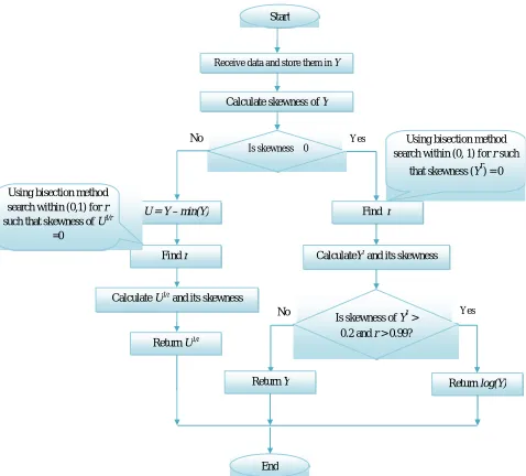
Finally, it should be mentioned that similar to the original Box-Cox transformation method, the original data of the proposed power transformation technique need to be positive. In this case, the absolute value of the minimum-valued data should be added to all to make them non-negatives. In summary the flowchart of the proposed algorithm is shown in Figure 1.
3. SIMULATION EXPERIMENTS
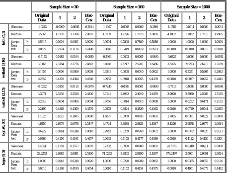
In order to investigate the performance of the proposed procedure and to compare it with the one of the complicated well-known Box-Cox transformation, simulation experiments have been conducted. In the simulation study, four different probability distributions of gamma, beta, weibull, and lognormal were used to produce all major types of non-normal skewed data. The simulation experiments are categorized into four classes of right-skewed, slightly-skewed, left-skewed, and logarithmic.
The first and the second rows of the smaller tables show the skewness and the kurtosis of the data, respectively. The third and the fourth rows of these tables show the results of JB-test (Jarque Bera) for each column. The third row shows the average value of the test statistics (h is zero if the normality hypothesis is accepted, and one if rejected) for 10000 runs, and the fourth row is the average of the p-values. The less the third-row value, and the more the fourth-row value are, the better is the performance of the corresponding
treatment. Hence, we can use these two values as measures of performances to describe and compare the effectiveness of the treatments.
The results of both Tables 1 and 2 show that the proposed power transformation method performs quite well in all right-skewed, left-skewed and logarithmic distributions and transforms non-normal data to non-normal data efficiently in almost all cases (in most cases treatment 2 provides better results than those of treatment 1). The Box-Cox method also performs well and does slightly better
Using bisection method search within (0, 1) for r such
that skewness (Yr) = 0
Return log(Y)
Start
Is skewness ≥ 0
Receive data and store them in Y
CalculateYr and its skewness
Is skewness of Yr > 0.2 and r > 0.99? Calculate skewness of Y
Find r U = Y – min(Y)
Find r
Using bisection method search within (0,1) for r
such that skewness of U1/r
=0
Calculate U1/r and its skewness
Return U1/r
Yes
No
Yes
No
Return Y
End
than the proposed procedure for small sample sizes. In medium and large sample sizes, even treatment 1 performs better than the Box-Cox method. However, the difference is not significant. Combining this finding with the ease of understanding and conducting of the proposed method, one may conclude that the proposed procedure provides a better approach for practical applications.
4. CONCLUSIONS
In this paper, the power transformation technique thatwas developed by Niaki, et al [1] was extended to transform right and left skewed distributions to distributions that are closer to normal. The value of the power was searched such that the skewness of transformed data becomes almost zero with an acceptable error. The performance of the proposed method was then compared to the ones of the well-known and complicated Box-Cox transformation method for different left-skewed, right-skewed and logarithmic distributions using Monte Carlo simulation. Besides simplicity in understanding and
implementing, the results of the simulation study showed that the proposed method works well, and is quite compatible to the complicated method of Box, et al [2] in all of the simulated experiments. Although the p-values of the normality tests of the Box-Cox method are slightly more than the ones obtained by the proposed procedure, the simplicity of the latter method makes it preferable especially when large data are treated.
5. REFERENCES
1. Niaki, S.T.A. and Abbasi, B., “Skewness Reduction
Approach in Multi-Attribute Process Monitoring”,
Communications in Statistics-Theory and Methods,
Vol. 36, (2007), 2313-2325.
2. Box, G. and Cox, D.R., “An analysis of Transformation”,
Journal of Royal Statistical Society B, Vol. 26, (1964),
211–243.
3. Manly, B.F.J., “Exponential Data Transformations”,
Statistician, Vol. 25, (1976), 37-42.
4. Li, P., “Box-Cox Transformations: An Overview”,
Technical Report (2005), on the web: http://www. stat. uconn.edu/~studentjournal/index_files/pengfi_s05.pdf.
5. John, J.A. and Draper, N.R., “An Alternative Family of
Transformations”, Applied Statistics, (1980), Vol. 29,
(1980), 190-197.
TABLE 1. Results of Simulation in 10,000 Replications of Right-Skewed Distributions.
Sample Size = 30 Sample Size = 100 Sample Size = 1000
Original
Data 1 2
Box-Cox
Original
Data 1 2
Box-Cox
Original
Data 1 2
Box-Cox
ga
mm
a
(2
,
2
) Skewness 1.0884 0.1500 0.1491 -0.0403 1.2854 0.0100 0.0097 -0.0231 1.3980 0.0008 -0.0004 -0.0135 Kurtosis 4.1470 2.8407 2.8401 2.5405 5.1440 2.7700 2.7692 2.7491 5.8738 2.8515 2.8508 2.8535
Jarque-Bera test
h 0.5783 0.0868 0.0866 0.0013 0.9950 0.0076 0.0077 0.0020 1.0000 0.0279 0.0254 0.0245
p 0.0756 0.4221 0.4222 0.4621 0.0044 0.4508 0.4515 0.4546 0.0010 0.3866 0.3926 0.3939
ga
mm
a
(1
,
2
) Skewness 1.4788 0.0775 0.0765 -0.0682 1.7868 0.0020 0.0004 -0.0489 1.9725 0.0004 -0.0001 -0.0392 Kurtosis 5.2355 2.6568 2.6562 2.4833 7.1596 2.6488 2.6397 2.6504 8.7169 2.7105 2.7093 2.7199
Jarque-Bera test
h 0.8203 0.0373 0.0373 0.0005 1.0000 0.0011 0.0009 0.0008 1.0000 0.2179 0.2100 0.2074
p 0.0269 0.4412 0.4414 0.4576 0.0013 0.4346 0.4353 0.4356 0.0010 0.2013 0.2081 0.2069
W
ei
bu
ll
(1
.5
,3
) Skewness 0.1359 -0.0515 -0.0530 -0.0683 0.1546 -0.0292 -0.0251 -0.0494 0.1674 -0.0014 -0.0002 -0.0392 Kurtosis 2.6184 2.5437 2.5435 2.4814 2.6981 2.6508 2.6486 2.6510 2.7259 2.7100 2.7088 2.7193
Jarque-Bera test
h 0.0311 0.0140 0.0140 0.0005 0.0357 0.0012 0.0009 0.0006 0.8291 0.2192 0.2113 0.2072
p 0.3755 0.4316 0.4317 0.4581 0.3319 0.4310 0.4313 0.4358 0.0318 0.2009 0.2067 0.2055
b
et
a
(2
,2
) (
sli
g
h
tl
y
ri
g
h
t s
k
ew
ed)
Skewness -0.0026 -0.1074 -0.1087 -0.1560 0.0012 -0.0679 -0.0602 -0.1506 -0.0002 -0.0146 -0.0205 -0.1493 Kurtosis 2.1793 2.1756 2.1764 2.1816 2.1562 2.1697 2.1667 2.2144 2.1442 2.1484 2.1499 2.2205
Jarque-Bera test
h 0.0016 0.0013 0.0013 0.0000 0.0434 0.0312 0.0319 0.0244 1.0000 1.0000 1.0000 1.0000
6. Bickel, P.J. and Doksum, K.A., “An Analysis of
Transformations Revisited”, Journal of the American
Statistical Association, Vol. 76, (1981), 296-311.
7. Yeo, I.K. and Johnson, R., “A New Family of Power
Transformations to Improve Normality or Symmetry”,
Biometrika, Vol. 87, (2000), 954-959.
8. Perri chi, L. R., “A Bayesian Approach t o
Transformations to Normality”, Biometrika, Vol. 68,
(1981), 35-43.
9. Sweeting, T.J., “On the Choice of Prior Distribution for
the Box-Cox Transformed Linear Model”, Biometrika,
Vol. 71, (1984), 127–134.
10. Hinkley, D.V. and Runger, G., “The Analysis of
Transformed Data”, Journal of the American Statistical
Association, Vol. 79, (1984), 302–309.
11. Cook, R.D. and Weisberg, S., “Applied Regression
Including Computing and Graphics”, Wiley, New York, U.S.A., (1999).
TABLE 2. Results of Simulation in 10,000 Replications of Left-Skewed and Logarithmic Distributions.
Sample Size = 30 Sample Size = 100 Sample Size = 1000
Original
Data 1 2
Box-Cox
Original
Data 1 2
Box-Cox
Original
Data 1 2
Box-Cox
b
et
a
(5
,1
)
Skewness -1.0243 -0.0009 -0.0005 -0.2814 -1.1367 -0.0008 0.0000 -0.2891 -1.1782 -0.0014 0.0000 -0.2911 Kurtosis 3.5865 1.7770 1.7764 2.0055 4.0139 1.7726 1.7715 2.0005 4.1802 1.7832 1.7818 1.9965
Jarque-Bera test
h 0.5615 0.0001 0.0001 0.0000 0.9994 0.7808 0.7809 0.5886 1.0000 1.0000 1.0000 1.0000
p 0.0627 0.2174 0.2176 0.2498 0.0046 0.0419 0.0419 0.0523 0.0010 0.0010 0.0010 0.0010
w
ei
bu
ll
(3
,10
) Skewness -0.5173 0.0185 0.0194 -0.0680 -0.5963 0.0003 0.0005 -0.0490 -0.6322 -0.0006 0.0000 -0.0392 Kurtosis 3.1165 2.3784 2.3776 2.4842 3.4046 2.5217 2.5207 2.6486 3.5495 2.6223 2.6210 2.7189
Jarque-Bera test
h 0.1955 0.0006 0.0006 0.0008 0.5531 0.0008 0.0010 0.0002 1.0000 0.5351 0.5267 0.2063
p 0.2557 0.4393 0.4394 0.4586 0.0955 0.3948 0.3955 0.4370 0.0010 0.0927 0.0957 0.2045
w
ei
bu
ll
(2
,15
) Skewness -0.6222 0.0105 0.0115 -0.0679 -0.7245 -0.0008 0.0001 -0.0490 -0.7813 -0.0008 0.0000 -0.0394 Kurtosis 3.3074 2.3536 2.3526 2.4830 3.7141 2.4932 2.4919 2.6470 3.9690 2.5980 2.5968 2.7185
Jarque-Bera test
h 0.2643 0.0004 0.0004 0.0004 0.7056 0.0014 0.0013 0.0008 1.0000 0.6252 0.6171 0.2132
p 0.2199 0.4368 0.4369 0.4576 0.0578 0.3824 0.3829 0.4362 0.0010 0.0719 0.0741 0.2055
log
n
(0
,
0
.5
) Skewness 1.1825 0.1625 0.1605 0.0008 1.4875 0.0969 0.0935 0.0001 1.7085 0.0391 0.0322 0.0000 Kurtosis 4.6450 2.6979 2.6978 2.5847 6.4724 2.8838 2.8833 2.8347 8.4256 2.9878 2.9875 2.9814
Jarque-Bera test
h 0.6222 0.0244 0.0244 0.0018 0.9942 0.0269 0.0268 0.0072 1.0000 0.0332 0.0326 0.0123
p 0.0760 0.4190 0.4191 0.4657 0.0035 0.4175 0.4177 0.4589 0.0010 0.4112 0.4136 0.4501
log
n
(0
,
5
)
Skewness 4.4544 0.1581 0.1557 0.0003 8.2382 0.0930 0.0900 0.0001 24.7876 0.0240 0.0211 0.0000 Kurtosis 22.2253 2.6885 2.6881 2.5800 74.0223 2.8892 2.8890 2.8397 678.2497 2.9901 2.9901 2.9824
Jarque-Bera test
h 1.0000 0.0248 0.0248 0.0020 1.0000 0.0290 0.0289 0.0062 1.0000 0.0355 0.0353 0.0136