The Analysis of Bayesian Probit Regression of Binary and Polychotomous Response Data

THE ANALYSIS OF BAYESIAN PROBIT REGRESSION OF

BINARY AND POLYCHOTOMOUS RESPONSE DATA

Shadi Nasrollahzadeh

Department of Mathematics, Teachers’ Training Faculty Tehran South Branch, Islamic Azad University

Tehran, Iran [email protected]

(Received: February 17, 2007 – Accepted in Revised Form: September 13, 2007)

Abstract The goal of this study is to introduce a statistical method regarding the analysis of specific latent data for regression analysis of the discrete data and to build a relation between a probit regression model (related to the discrete response) and normal linear regression model (related to the latent data of continuous response). This method provides precise inferences on binary and multinomial models which particularly in the case of small samples, has preference to maximum likelihood methods. The probit regression model for binary outcomes can be easily and precisely explained using different normal distributions for latent data modeling. Applying this approach and using Gibbs sampler method needs simulation of standard distributions such as multivariate normal distribution. Therefore, it can be easily implemented by many softwares and it provides a general method for analyzing binary (or polychotomous) response regression models.

Keywords Regression, Binary Probit, Data Augmentation, Gibbs Sampling, Hierarchical Bayes Modeling, Latent Data, Multinomial Probit, Residual Analysis, Student-t Link Function

ﻩﺪﻴﻜﭼ

ﻩﺩﺍﺩ ﺯﺍ ﻩﺩﺎﻔﺘﺳﺍ ﻪﺑ ﻁﻮﺑﺮﻣ ﻱﺭﺎﻣﺁ ﺵﻭﺭ ﻲﻓﺮﻌﻣ ﻪﻟﺎﻘﻣ ﻦﻳﺍ ﺯﺍ ﻑﺪﻫ ﻞﻴﻠﺤﺗ ﻱﺍﺮﺑ ﺹﺎﺧ ﻲﻧﺎﻬﻧ ﻱﺎﻫ

ﻩﺩﺍﺩ ﻲﻧﻮﻴﺳﺮﮔﺭ ﺖﻴﺑﻭﺮﭘ ﻥﻮﻴﺳﺮﮔﺭ ﻝﺪﻣ ﻦﻴﺑ ﻁﺎﺒﺗﺭﺍ ﻱﺭﺍﺮﻗﺮﺑ ﻭ ﻪﺘﺴﺴﮔ ﻱﺎﻫ

) ﻪﺘﺴﺴﮔ ﺦﺳﺎﭘﻪﺑ ﻁﻮﺑﺮﻣ (

ﻝﺪﻣ ﻭ

ﻝﺎﻣﺮﻧﻲﻄﺧﻥﻮﻴﺳﺮﮔﺭ )

ﻩﺩﺍﺩﻪﺑﻁﻮﺑﺮﻣ ﻪﺘﺳﻮﻴﭘﺦﺳﺎﭘﻲﻧﺎﻬﻧﻱﺎﻫ

( ﺖﺳﺍ . ﺵﻭﺭ ﻦﻳﺍ ﻲﻣﻥﺎﻜﻣﺍ

ﻁﺎﺒﻨﺘﺳﺍﻪﻛﺪﻫﺩ ﻱﺎﻫ

ﻝﺪﻣﻱﺍﺮﺑﻲﻘﻴﻗﺩ ﻪﻧﻮﻤﻧ ﺭﺩﻩﮋﻳﻭﻪﺑﻪﻛﻢﻴﻫﺩﻡﺎﺠﻧﺍﻲﺘﻟﺎﺣﺪﻨﭼﻭﻲﺘﻟﺎﺣﻭﺩﻥﻮﻴﺳﺮﮔﺭﻱﺎﻫ

ﺵﻭﺭﻪﺑ،ﻚﭼﻮﻛﻱﺎﻫ

ﺖﺳﺭﺩﺮﺜﻛﺍﺪﺣ ﺩﺭﺍﺩﻱﺮﺗﺮﺑﻲﻳﺎﻤﻧ

. ﻊﻳﺯﻮﺗﺯﺍﻩﺩﺎﻔﺘﺳﺍﺎﺑﺍﺭﻲﺘﻟﺎﺣﻭﺩﺞﻳﺎﺘﻧﻱﺍﺮﺑﺖﻴﺑﻭﺮﭘﻥﻮﻴﺳﺮﮔﺭﻝﺪﻣ ﻝﺎﻣﺮﻧﻱﺎﻫ

ﻩﺩﺍﺩﻱﺪﻨﺑﻝﺪﻣﻱﺍﺮﺑﻒﻠﺘﺨﻣ ﻧﺎﻬﻧﻱﺎﻫ

ﻲﻣﺖﻗﺩﺎﺑﻭﻲﻧﺎﺳﺁﻪﺑﻲ ﺩﺮﻛﻪﻴﺟﻮﺗﻥﺍﻮﺗ

. ﺯﺍﻩﺩﺎﻔﺘﺳﺍﻭﺭﺍﺰﺑﺍﻦﻳﺍﻱﺮﻴﮔﺭﺎﻜﺑ

ﻪﻧﻮﻤﻧﺵﻭﺭ ﻊﻳﺯﻮﺗﻱﺯﺎﺳﻪﻴﺒﺷﻪﺑﺰﺒﻴﮔﺮﻴﮔ

ﻥﺁﻱﺍﺮﺟﺍﻪﻛﺩﺭﺍﺩﺯﺎﻴﻧﻩﺮﻴﻐﺘﻣﺪﻨﭼﻝﺎﻣﺮﻧ ﻊﻳﺯﻮﺗﺪﻨﻧﺎﻣﺩﺭﺍﺪﻧﺎﺘﺳﺍﻱﺎﻫ

ﻡﺮﻧﺯﺍ ﻱﺭﺎﻴﺴﺑ ﺯﺍﻩﺩﺎﻔﺘﺳﺍ ﺎﺑ ﻭﻞﻴﻠﺤﺗ ﻱﺍﺮﺑ ﺍﺭﻡﺎﻋ ﻲﺷﻭﺭ ﻭﺖﺳﺍ ﻥﺎﺳﺁ ﻱﺮﺗﻮﻴﭙﻣﺎﻛ ﻱﺎﻫﺭﺍﺰﻓﺍ

ﻝﺪﻣﻲﺳﺭﺮﺑ ﻱﺎﻫ

ﻲﺘﻟﺎﺣﻭﺩﺦﺳﺎﭘﻥﻮﻴﺳﺮﮔﺭ )

ﻲﺘﻟﺎﺣﺪﻨﭼﻭ (

ﻲﻣﻢﻫﺍﺮﻓ ﺩﺯﺎﺳ .

1. INTRODUCTION

A vast literature in statistics, biometrics, and econometrics is concerned with the analysis of binary and polychotomous response data. For example in pharmacognosia tests, after using different viscosity of special poison on limited time duration, the researchers count the dead insects and they often want to find the best relation between the ratio of death and viscosity of poison. In statistical researches when independent variables and dependent variables (response) are continuous, regression methods are used. If independent variables are discrete and response variables are continuous the analysis of variance

methods, and if some of the independent variables are discrete and the others, continuous, the analysis of covariance methods will be used.

But, in cases where the response variable is discrete (regardless of the type of independent variables), nonlinear methods are used. These are the main parts of statistical researches, especially those in the biometry field. As, these investigations are very important in applied sciences, their analysis methods will be discussed.

(classic, Bayesian and maximum likelihood), because of their special defection [1].

The regression relation of dependent variable Y in terms of one or several independent variables X is E(Y|X) = XB. In the case of binary discrete response variable instead of data, different probabilities are considered proper non linear model for regression relation is used. These nonlinear models are shown as: E(Y|X) = P(Y=1) = P = H(X)

H(.) is a certain cumulative distribution function called link function and it links conditional expectations of variable Y to the independent variable(s) X. If in nonlinear regression models for discrete data, the variation of Y in terms of X is approximately logarithmic, then H is considered as standard normal cumulative distribution function (Φ) and the probit model is obtained, whereas the logit model is obtained if H is the logistic cdf [2]. If N is observed independently of the binary random variables yi (i=1,…N) with success

probabilities Pi (Pi parameters are related to the

discrete or continuous auxiliary variables by link function), the binary probit regression model is defined as follows

i u ) i x ( i

y =Φ ′β + ⇒

N ,..., 1 i ) i x ( i P ) i x i y (

E = =Φ ′β =

Where

⎪⎩ ⎪ ⎨ ⎧

= β

′ Φ −

= β

′ Φ − =

0 i y if ) i x (

1 i y if ) i x ( 1 i u

So, the residuals do not have sufficient information to define outliers. While in (normal) Bayesian regression models, the residuals have a continuous distribution on an interval, and they are more efficient to define the outliners;

) 2 i , o ( N ~ i , ) 2 i , i x ( N ~ i Z

N ,.., 1 i i i x i Z

σ ε

σ β ′

= ε

+ β ′ =

Consequently, a relation is made between the binary probit regression models and (normal) Bayesian regression models. In this paper, a method is introduced to estimate regression

coefficients vector (β), with iterated sampling of (standard or nonstandard) conditional distributions, through the Bayesian methods under normal linear regression model. The Gibbs sampler is a modification of the Metropolis algorithm [3]. The Metropolis algorithm was developed to investigate the equilibrium properties of large systems of particles such as molecules in a gas.

Hasting [4] suggests Markov’s chain methods of sampling that generalize the Metropolis algorithm. Li [5,6] appears to have independently developed the Gibbs sampler in the context of multiple imputation. In this paper the Gibbs sampler algorithm is used with a focus on its implementation in the binary and polychotomous reponse models [7]. This approach is very similar to the data augmentation formework used in cencored regression models [8].

If in Bayesian analysis for attaining effect estimation, minimizing the E(βˆ−β)2 is considered, the final estimation would be the posterior distribution mean. Then, the polynomial probabilities are estimated by the relation between these probabilities and the linear combination of regression coefficients.

As an application, the analysis of the Bayesian regression method regarding effects of fourteen different environments on relative frequency of five kinds of special insects, based on the results of a real experience, is mentioned in this paper.

2. BAYESIAN PROBIT REGRESSION

using mixtures of normal distributions to model the latent data [10] (the mixtures of normal distributions are normal distributions that their means and variances, or both are definite function of random variables with specific distributions). In this normal mixture class, one can investigate the sensitivity of the parameter estimates to the choice of "link function". The method can also be generalized to multinomial response models.

3. THE GIBBS SAMPLER

An algorithm for extracting the marginal distributions from these full conditional distributions was formally introduced by Geman and Geman (1984) [11,12].

The Gibbs sampler was developed and has been mainly applied in the context of complex stochastic models involving very large numbers of variables [13]. The Gibbs sampling is a Markovian updating scheme that proceeds as follows:

Given an arbitrary starting set of values ) 0 ( k U ,..., ) 0 ( 1 U

Observation U₁(1) from

) ) 0 ( K U ,..., ) 0 ( 2 U | 1 U (

π observation U(₂1) from

) ) 0 ( K U ,..., ) 0 ( 3 U , ) 1 ( 1 U | 2 U (

π …

and

observation U(_k1) from π(U_K|U₁(1),U(₂1),...,U(_K0)₋₁) will be produced.

3.1. Convergence

(Densities are denoted

generically by brackets). ] K U ,..., 1 U [ d ) ) i ( k U ,..., ) i ( 1 U ( ⎯⎯→

and hence for each S if i→∞ ] S U [ ~ S U d ) i ( S

U ⎯⎯→

The Gibbs sampling through m replications of the aforementioned i iterations produces m iid k tuples (U₁(i_j),U(₂i_j),...,U_kj(i)) (j=1,2,…,m), with the proposed density estimate for [US] having form

∑ = = ≠ = m 1 j ] s t ; i ) tj ( U t U | S U [ m 1 i ] S Uˆ [

4. DATA AUGMENTATION AND GIBBS SAMPLING FOR BINARY DATA

Introduce N latent variables Z1,…, ZN where the Zi

are independent N(x'iβ, 1) and [14] define Yi = 1 if

Zi > o and Yi = 0 otherwise. Then, ~Ber(P_i)

id i Y = β ′ − > = > = =

=P(Y_i 1) P(Z_i 0) P(U x_i )

i P ) i x ( ) i x U (

P < ′β =Φ ′β

So, the Zi, given the data yi follows a truncated

normal distribution. By introducing the Zi's in to

the model, the probit regression model on the Bernoulli observations Y is seen to have an underlying normal regression on Zi

) 1 , 0 ( N ~ i ; i i x i

Z = ′β+ε ε .

As an example [15], consider binary probit regression on target variables y_n∈

{ }

0,1 , the probit likelihood for the nth data sample taking unit value (yn=1) is P(yn=1|xn,β) =Φ(x_n′β). Now, this can be

obtained by the following marginalization

n dz ) , n x | n Z ( p ) n Z | 1 n y ( P n dZ ) , n x | n Z , 1 n y ( p β = ∫ = β = ∫

and as by definition p(y_n =1|Z_n)=δ(Z_n >0) then it can be seen that the required marginal is simply the normalizing constant of a left truncated univariate Gaussian so that

. ) n x ( n Z d ) 1 , n x ( n Z N ) 0 n Z ( ) ) , n x | 1 n y ( P β ′ Φ = β ′ > δ ∫ = β =

joint distribution

) 1 , n x ( n Z N ) 0 n Z ( ) , n x | n Z , 1 n y (

P = β =δ > ′ β

provides a straightforward means of Gibbs sampling from the parameter posterior which would not be the case if the marginal term,

) n x ( ′β

Φ , was employed in defining the joint distribution over data and parameters.

This data augmentation strategy can be adopted in developing efficient methods to obtain binary and multi-class Gaussian process (GP) classifiers [16]. By computation of the marginal posterior distribution of β using the Gibbs sampling algorithm requires only the posterior distribution of

β conditional on Z and the posterior distribution of Z conditional on β, and these fully conditional distributions are of standard forms

∏

= Φ ′β

β π = β

π N

1 i

) 1 , i x ; i Z ( ) ( C ) Z , Y | (

If a priori the distribution of β is diffuse, then )

1 ) X X ( ), Z X ( 1 ) X X (( K N ~ Z , Y

| ′ − ′ ′ −

β

If β is assigned the proper conjugate N(β*_,B*₎

prior, then the posterior distribution of β given Z is Nk(β~,B~).

where

) Z X * * B ( 1 ) X X 1 * B (

~₌ − _{+ ′} − _{β + ′}

β

1 ) X X 1 * B ( B

~ ₌ − _{+ ′} −

The posterior of Z, conditional on β, also has a simple form truncated normal distribution as follow:

Zi | y, β distributed N(x'iβ,1)

Truncated at the left by o if yi = 1

Zi | y, β distributed N(x'iβ,1)

Truncated at the right by o if yi = o

Given a previous value of β, one cycle of the Gibbs algorithm would produce Z and β from the mentioned distributions. The starting value of β, β (o)

may be taken to be the maximum likelihood (ML) estimate, or the least squares (LS) estimate (x'x)-1

x'y.

Since the posterior distribution of β given Z is multivariate normal, it is possible to generalize this model by applying suitable mixtures of normal distributions.

For example, one can generalize the probit link by choosing the link cdf H to be the family of t distributions. Let Zi be independently distributed

from t distributions with locations x'_iβ, scale parameter 1 and degree of freedom r. the additional random variable λi is introduced and distributed

Gamma (r/2,2/r). Zi|λi is distributed N (x'_iβ,λi-1).

Suppose a uniform prior is chosen for β and λ = (λ1,…,λN) be the vector of scale parameters. The

fully conditional distributions of β, Z, λ and r are given below:

β|y, Z, λ, r ~ Nk(βˆ_z,λ,(X′WX)−1)

Where

) i ( diag W , ) Z 1 W X ( 1 ) WX X ( , z

ˆ _{= ′} − _′ − _{= λ}

λ β

) 1 i , i x ( N ~ r , , , y | i

Z βλ ′β λ−

Truncated at the left by o if yi = 1

) 1 i , i x ( N ~ r , , , y | i

Z βλ ′β λ−

Truncated at the right by o if yi = o

) 2 ) ' i x i Z ( r

2 ,

2 1 r ( Gamma ~ r , , Z , y | i

β − + + β

λ r|y, Z, β,

λ is distributed according to the pdf proportional to Where

1 2 r ) 2 r ( ) 2 r ( ) r ( C

−

⎥ ⎥ ⎥

⎦ ⎤

⎢ ⎢ ⎢

and π(r)is the prior on r.

It started with βˆ=(X′X)−1X′y(LSE),setλ_i =1 for all i, and cycle through the conditional distributions Z, β, λ, r, in that order.

For making inferences about the regression vector β and the probabilities

). ) i ( , ) i ( Z | ( m

1 i m

1 ) ( ˆ by

ed approximat is

for posterior The

, k P

λ β π ∑ = ≈ β π

β ⎭

⎬ ⎫ ⎩ ⎨ ⎧

To obtain a posterior density estimate for Pk, it is

known that

Pk = 2 x_k ).

1

k

(λ ′ β

Φ

Then by a transformation, the density estimate of the probability is given by

) k P ( 1 ( / ) 2 , ); k P ( 1 ( m

1 i m

1 ) k P (

ˆ ∑ φ Φ− μσ φ Φ−

= =

π ; o,1)

Where

) 2 , ( N the is ) 2 , ;

( μσ μσ

φ pdf, μ= λ(_ki) x′_kβˆ_z,λ

and

k x 1 ) WX X ( k x ) i (

k

2 _{=λ ′ ′} −

σ

5. GENERALIZATION TO A MULTINOMIAL RESPONSE

The data with multinomial distribution is called polychotomous response data. Each yi can be

considered as a special category. Then there are two different situations, multinomial probit model with

5.1. Orderd Categories 5.2. Unordered Categories

5.1. Ordered Categories

Suppose that y1,…,

yN are observed, where yi takes one of J ordered

categories, 1,…, J. and

J ,..., 2 , 1 j

N ,..., 2 , 1 i )

j i Y ( p ij P

= = =

=

The cumulative probabilities are defined

∑

= = −

=

ξ j

1 k

1 J ,..., 2 , 1 j ik

p ij

The latent continuous random variable Zi

distributed N(x_i′β,1)

and yi is observed Where yi= j if γ_j−1<Z_i≤γ_j

) 0 , J

(γ =∞ γ =−∞ . Then the regression model for the

{ }

P_ij is given by ξ_ij=Φ(γ_j−x_i′β).

If a diffuse prior for (β,γ), is assigned then )

1 , i x ( N ~ j i Y , , | i

Z βγ = ′β truncated at the left (right) by 1

j−

γ (γ_j). Finally, γj given Z, y, β can be seen to

be uniform on the specified interval. To implement the Gibbs sampler, start with (β,γ) set equal to the MLE and simulate form mentioned distributions. After getting the result of Bayes estimate of β

(posterior distribution mean) and using normal regression model

) i x j ( ij=Φ γ − ′β

ξ

polynomial probabilities

{ }

P_ij can be calculated.

5.2. Unordered Categories

Probit model for

polynomial data is considered as follows

) i x ( ij

P =Φ ′β

J ,..., 2 , 1 j

N ,..., 2 , 1 i

= =

i is the index of experimental units and j is the index of categories. In unit i, one of the possible J results with probabilities of Pi1,…,PiJ observed.

Latent data Zi = (Zi1,…,ZiJ) was introduced and

J ,..., 2 , 1 j N ,..., 2 , 1 i = =

Z

_ij

=

x

_ij

′

β

+

ε

_ij

) ij ,..., 1 i (

i= ε ε ′

ε Where ) , 0 ( J

N Σ is distributed

Σ

is a JxJ matrix that is parameterized in terms of parameter vector θ of dimension not exceeding

2 ) 1 J ( J − .

Category j is observed if Zij > Zik and the

multinomial probabilities are given by > ε + β ′ = ≠ ∀ >

=P(Z_ij Z_ik ; k j) P(x_{ij ij} ij

P

So, computation of these probabilities entails calculation of multiple integrals of the multivariate normal density; thus maximum likelihood estimation is very difficult to perform for Large J. By the following the Gibbs sampling approach, the computation of the multinomial probabilities can be avoided. The vector of observed categories is denoted as Y = (y1,…,yN) where yi ∈

{

1,....,J

}

and xi = (xi1,…., xiJ)′, the preceding model can be

rewritten as

Z = Xβ + ε where ε = (ε′₁,...,ε′_N)′is distributed N_NJ(o,Ω=I_N⊗∑).

The operator ⊗ is the direct multiplication of two matrixes and it is defined as follow

⎥ ⎥ ⎥ ⎥ ⎦ ⎤ ⎢ ⎢ ⎢ ⎢ ⎣ ⎡ = × ⊗ × = B pp a ... B 1 p a B p 1 a ... B 11 a n n B P P A C _M

To implement the Gibbs sampler, samples are required to form the following conditional distributions: β θ θ β θ β , N Z ,..., 1 Z , Y | , , Y | N Z .., ., 1 Z , N Z ,..., 1 Z , Y |

If a diffuse prior is placed on β, then standard multivariate normal theory yields that

) 1 ) X 1 X ( , Z ˆ ( K N ~ , Y , N Z ..., , 1 Z

| θ β ′Ω− −

β where

) Z 1 X ( 1 ) X 1 X ( z

ˆ _{= ′Ω}− − _′Ω−

β

The vector

{ }

Z_i given Y, β, θ is an independent collection with T2 =nβ′ˆ₁S₁−1β′ˆ₁=324.16 _{such that} the yi th component of Zi is the maximum. Using a

prior π(θ)onθ, the density of this distribution is proportional to ⎭ ⎬ ⎫ ⎩ ⎨

⎧− _{− β′Ω}− _{θ − β}

− θ Ω θ π = θ ) X Z ( ) ( 1 ) X Z ( 2 1 exp 2 1 | ) ( | ) ( ) ( f

This distribution is not a familiar parametric family and is relatively difficult to simulate. However, in Bayesian methods, the conditional distribution mode can be introduced as an estimation, after calculating the posterior distribution. The considered mode can be calculated by using the methods of differentiating of matrix functions [17] as follows o 2 1 | ) ( | ) X Z ( ) ( 1 ) X Z ( 2 1 exp ) ( 1 ) X Z ( ) X Z ( ) ( 1 2 1 ) X Z ( ) ( 1 ) X Z ( 2 1 exp ) ( 1 | ) ( | 2 3 | ) ( | 2 1 ) ( f = − θ Ω ⎭ ⎬ ⎫ ⎩ ⎨

⎧− _{− β′Ω}− _{θ − β}

θ − Ω ′ β − β − θ − Ω + ⎭ ⎬ ⎫ ⎩ ⎨

⎧− _{− β ′Ω}− _{θ − β}

θ − Ω θ Ω − θ Ω − = θ ∂ θ ∂ ⎭ ⎬ ⎫ ⎩ ⎨

⎧− _{− β′Ω}− _{θ − β}

θ − Ω − θ Ω − ⇒ ) X Z ( ) ( 1 ) X Z ( 2 1 exp ) ( 1 2 1 | ) ( | 2 1

)

o ( 1 ) X Z ( ) X Z ( I

( − − β − β′Ω− θ =

o ) ( 1 ) X Z ( ) X Z (

I− − β − β′Ω− θ = ⇒ o ) X Z ( ) X Z ( )

(θ − − β − β′= Ω ⇒ ) X Z ( ) X Z ( ) (

ˆ _{θ = − β − β′}

So, one way for estimating θ is to calculate Ri = Zi

-Xiβ and R_iR_i

^

i = ′

∑ in each of the implementation of

the Gibbs sampler. Then the estimation of matix ∑

can be the arithmetic average of ∑^_i for i = 1,….,N.

Considering the initial values I ) o ( ^

=

∑ and

) Y 1 X ( 1 ) X 1 X ( ) o (

ˆ _{= ′Ω}− − _′Ω−

β , the samplings

implement of the fully conditionally distributions in the order of Z, β, θ (and calculate the estimation of ∑ in each time). After implementing the Gibbs sampler with the different initial points m = m*, which are iterated t = t* times, the mean and variance of the marginal posterior distributions could be calculated and the average of vectors can be introduced as Bayes estimation [18]. Incidentally, in the most of the practical cases t ≤

50 and m ≤ 100 were proper for convergence.

6. A NUMERICAL EXAMPLE

6.1. Experiment and Design

Although it has

been well documented that coarse woody debris are important in temperate forest ecosystems, little is known on whether or not these debris have any effect on maintaining biodiversity. Thus, the following experiment was conducted in order to find whether or not decaying logs provide microhabitat for the different species of ground-dwelling arthropods. On the upper coastal plain of Georgia, a twelve month study was undertaken at two adjacent sites on the Savanna River Site [19]. Hundreds of species were collected each month. The dataset contained the following variables (with their respective meanings).The first factor has two levels:

• MH (Mixed Hardwood)

• PP (Pine)

The second factor has seven levels:

• F (Fake Log)

• CD (Control Dry)

• CW (Control Wet)

• GD (Green Log Dry)

• GW (Green Log Wet)

• DD (Decomposed Log Dry)

• DW (Decomposed Log Wet) The third factor has six levels:

• COLL (Number of collembola collected)

• COLEOP (Number of coleopterans collected)

• HYMEN (Number of hymenpterans collected)

• SPID (Number of spiders collected)

• ORTHOP (Number of orthopterans collected)

• MISC (Number of miscellaneous ground bugs collected)

Five replications were done for each situation.

6.2. Analysis

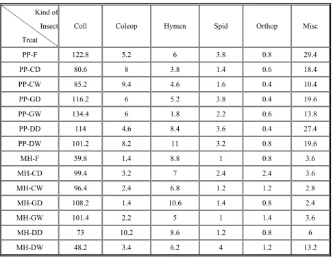
For analyzing this experiment,

fourteen combinations of treatments (2×7) and species of ground-dwelling arthropods were considered as independent variable and the number of species as dependent variable. The dataset of the first month are shown in Table 1.

The five replications of observations in the first cell in Table 1 have been 207, 121, 55, 157, 74, therefore the expected number in this cell is 122.8. The vector of observations Y is the number of observations collected from treatments.

This vector is Y = (y'1,…,y'14)' where y =

(yi1,…yi6)', and each category has the average of

five replications.

Vector Z also has the same form. The linear normal regression model is considered

Zij = x'ijβ+

ε

ij i = 1,…,14j = 1,…,6

or in matrix form Z = Xβ + ε where ε = (ε′₁,...,ε′₁₄) is distributed N₈₄(o,Ω) (Ω=I₁₄⊗∑₆ ) and εI =

) 6 i ,..., 1 i

(ε ε ′ is distributed N₆(o,∑ ).

The regression coefficients β has the following form

β = (βo,β1,…,β5,β6,β7,…,β18)'

Where βo is the constant of the model and βj (j =

6, ….., 18) shows the effect of the combination of treatment j on number of species.

The independent variables are discrete, the auxiliary variables Xi must be used. The matrix of

X (design matrix) is defined as

⎥ ⎥ ⎥ ⎥ ⎥ ⎥ ⎥ ⎥ ⎥ ⎥ ⎥ ⎥ ⎥

⎦ ⎤

⎢ ⎢ ⎢ ⎢ ⎢ ⎢ ⎢ ⎢ ⎢ ⎢ ⎢ ⎢ ⎢

⎣ ⎡

= ×

14 X . . .

2 X

1 X

19 84 X

and Xi is a 6×19 matrix with proper form. By using

the computer program prepared by the author of this paper for the mentioned method and iterating Gibbs sampler for t = 10, m = 40 the mean and variance-covariance matrix of marginal posterior distribution of β and the mean of posterior distribution as Bayes estimation have been calculated for each month. Incidentally, in addition to Bayes estimations, the calculated maximum likelihood estimations, for comparison, are shown in Table 2. It is well found that the results are reasonable and expected. Variance-covariance matrix S (19×19) ∑

∧

)

( _{also is}

calculated, but because of its large dimensions it has not been shown here.

TABLE 1. Expected Numbers of Insects in Month One. Kind of

Insect Treat

Coll Coleop Hymen Spid Orthop Misc

PP-F 122.8 5.2 6 3.8 0.8 29.4

PP-CD 80.6 8 3.8 1.4 0.6 18.4

PP-CW 85.2 9.4 4.6 1.6 0.4 10.4

PP-GD 116.2 6 5.2 3.8 0.4 19.6

PP-GW 134.4 6 1.8 2.2 0.6 13.8

PP-DD 114 4.6 8.4 3.6 0.4 27.4

PP-DW 101.2 8.2 11 3.2 0.8 19.6

MH-F 59.8 1.4 8.8 1 0.8 3.6

MH-CD 99.4 3.2 7 2.4 2.4 3.6

MH-CW 96.4 2.4 6.8 1.2 1.2 2.8

MH-GD 108.2 1.4 10.6 1.4 0.8 2.4

MH-GW 101.4 2.2 5 1 1.4 3.6

MH-DD 73 10.2 8.6 1.2 0.8 6

6.3. Hypothesis Testing

Regarding the results,

the following hypothesis testing and inferences can be performed:

6.3.1. For each month, hypothesis testing

⎪⎩ ⎪ ⎨ ⎧

≠ β

= β

o : 1 H

o : o H

has been considered where Ho is “The kind of

insects and different environments have no effect on the frequency of insects”.

As the matrix ∑ is unknown, matrix S is used. The critical region of Ho is

) P n , P ( F P n

P ) 1 n ( ) o ˆ ( 1 S )' o ˆ ( n 2

T _α −

− − > β − β − β − β =

Where

n = 40 P = 19 α=0.05 βo=o.

For example the value of test statistic T2 _{for the}

first month is

16 . 324 1 ˆ 1 1 S 1 ˆ n 2

T = β′ − β′ =

86 . 75 ) P n , P ( F P n

P ) 1 n

( _{− =}

α − −

TABLE 2. Estimations of Regression Coefficients in Month One.

ML Estimations Bayes Estimations

2.067 e + 000 1.909 e + 000

1.450 e + 001 1.431 e + 001

1.751 e + 000 1.635 e + 000

5.292 e + 000 5.194 e + 000

8.148 e – 001 7.513 e – 001

1.979 e – 001 8.187 e – 002

-2.931 e + 000 -2.776 e + 000

-1.261 e + 000 -1.055 e + 000

-2.523 e + 000 -2.325 e + 000

-1.883 e + 000 -1.401 e + 000

-1.474 e + 000 -1.085 e + 000

-3.204 e + 000 -2.883 e + 000

-2.078 e + 000 -1.907 e + 000

-2.037 e + 000 -1.986 e + 000

-3.434 e + 001 6.425 e – 002

2.452 e + 000 2.585 e + 000

-1.143 e + 000 -1.236 e + 000

1.498 e + 000 -1.231 e + 000

324.16 > 75.86 so, Ho is rejected.

6.3.2. For each month hypothesis testing

⎪⎩ ⎪ ⎨ ⎧

β ≠ β

β = β

o : 1 H

o : o H

Where

⎥ ⎥ ⎦ ⎤ ⎢

⎢ ⎣ ⎡

× β

× = β

1 13 1 ˆ

1 6 o o

has been considered that Ho is “The kind of insects

has no effect on the frequency of insects”.

T2=n(βˆ−β_o)'S−1(βˆ−β_o)=11895>75.86 so, Ho

is rejected.

6.3.3. Hypothesis testing for each level of factors;

For example in the fourth month:

⎪⎩ ⎪ ⎨ ⎧

≠ β

= β

o 7 : 1 H

o 7 : o H

where Ho is “The environment MH-F has no effect

on frequency of insects" (MH-F is the seventh regression coefficient in vector β).

Test statistic 1.218 17

. 5

77 . 2

7 ˆ S7

ˆ c

t = − =−

β β

= where

is in acceptance region −t(₀39_.025) <t<t(₀39_.025) therefore, Ho is accepted.

6.3.4. The hypothesis testing for comparing two different regression factors is considered as:

j ,i j i : 1 H

j i : o H

∀ ⎪⎩

⎪ ⎨ ⎧

β ≠ β

β = β

which with Δ=β_i−β_j is converted to equivalent test

⎪⎩ ⎪ ⎨ ⎧

≠ Δ

= Δ

o : 1 H

o : o H

. Statistic D=βˆ_i−βˆ_j is distributed

) j i 2 2

j 2 i , (

N Δ σ +σ − σ σ ~t(n 1)

D S

D c t

So = _α −

) j S i S 2 2 j S 2 i S 2 D S

( = + − and the critical region of Ho is t_c>t(_αn−1).

For example in the fifth month we can test

⎪⎩ ⎪ ⎨ ⎧

β > β

β = β

16 14 : 1 H

16 14 : o H

where H1 is “The PP-CW is more effective than

MH-DW on frequency of insects 612

. 0 16 ˆ 14 ˆ

D=β −β =

034 . 3 0408 . 0

613 . 0 c t 0408 . 0 2 D

S = → = =

) 39 (

05 . 0 t c t 68 . 1 ) 39 (

05 . 0

t = → >

Therefore, H1 is accepted.

For example in the fifth month these hypothesis testing can be performed for comparing each two desired factors.

7. CONCLUSION

The main novelty of this paper, has been that by introducing latent data into the problem, the probit model on the binary response is connected with the normal linear model on the continuous latent data reponse. A simulation-based approach has been introduced for Computing the exact posterior distribution of regression coefficients.

Applying this approach allows one to perform exact inference for binary regression models; this will likely be preferable to ML methods for small samples and is especially attractive in the multinomial setup, where it can be difficult to evaluate the likelihood function.

By using Gibbs sampling for simulation from standard distributions, one is introducing extra randomness into the estimation procedure and it is important to understand when a particular simulation process has converged.

augmentation method, also the ML estimations for comparison and some possible hypothesis testing for inference have been illustrated. Augmenting binary and polychotomous response models with Gaussian latent variables enables exact Bayesian analysis via Gibbs sampling from the parameter posterior.

Because the relative simplicity of this simulation method in this application, it is believed that there will be future research into the automation of this algorithm so that it can be incorporated into standard statistical software.

8. NOMENCULATURE

Ber: Bernoulli Distribution d: Distributed;

E: Expected Value;

F: Snedecor’s F Distribution; H0: Null Hypothesis;

H1: Alternative Hypothesis;

id: Independent Distributed; iid: Independent and Identically Distributed; N(μ,σ): The Normal Distribution with Mean μ

and Standard Deviation σ

P: Dimension of Vector β; S: Covariance Matrix of Sample; t: Student’s t Distribution; u: Residual;

) i ( k

U : K ‘th Observation of i ‘th Iteration;

Φ: Cumulative Distribution Function of Standard Normal Distribution;

β: Regression Coefficient Vector; βˆ: Estimation of β;

β0: Initial Value of β;

θ: The Unknown Vector Parameter of Dimension not Exceeding

2 ) 1 J ( J − _;

∑

: J Dimensional Covariance Matrix of

Population in Terms of θ;

ξ: Cumulative Probability;

α: Significance Level of a Test;

ε: Error of Estimation; )

(θ

Ω : NJ Dimensional Covariance Matrix of Population in Terms of θ;

9. REFERENCES

1. Zellner, A. and Rossi, P. E., “Bayesian Analysis of Dichotomous Quantal Response Models”, Journal of

Econometrics, Vol.25, (1984), 365-393.

2. Nelder, J. A. and McCullagh, P., “Generalized Linear Models”, Chapman and Hall, New York, U. S. A., (1989).

3. Metropolis, N., Rosenbluth, A. W., Rosenbluth, M. N., Teller, A. H. and Teller, E., “Equations of State Calculations by Fast Computing Machines”, Journal of

Chemical Physics, Vol.21, (1953), 1087-1091.

4. Hasting, W. k., “Monte Carlo Sampling Methods Using Markov Chains and Their Applications”, Biometrika,

Vol.57, (1970), 97-109.

5. Li, K. H., “Hypothesis Testing in Multiple Imputation with Emphasis on Mixed-up Frequencies in Contingency Tables”, Ph.D. Dissertation, University of Chicago, Chicago, U. S. A., (August 1985).

6. Li, K. H., “Imputation Using Markov Chains”, Journal

of Statistical Computation and Simulation, Vol. 30,

(1988), 57-79.

7. Albert, J. H. and Chib, S., “Bayesian Analysis of Binary and Polychotomous Response Data”, Journal of the

American Statistical Association,Vol. 88, (1993),

669-679.

8. Chib, S., “Bayes Inference in the Tobit Censored Regression Model”, Journal of Econometrics, Vol.51,

(1992), 79-99.

9. Khajeh Nouri, A., “Advanced Statistics and Biometry”, Tehran University Publicatian, Tehran, Iran, Chapter 18, (1969).

10. Wei, G. C. G. and Tanner, M. A., “Posterior Computations for Censored Regression Data”, Journal

of the American Statistical Association, Vol.85, No.

411, (1990), 829-839.

11. Gelfand, A. E. and Smith, A. F. M., “Sampling Based Approaches to Calculating Marginal Densities”,

Journal of the American Statistical Association, Vol.

85, (1990), 398-401.

12. Geman, S. and Geman, D., “Stochastic Relaxation, Gibbs Distributions and the Bayesian Restoration of Images”, IEEE Transactions on Pattern Analysis and

Machine Intelligence, Vol. 6, (1984), 721-741.

13. Zeger, S. L. and Karim, M. R., “Generalized Linear Models with Random Effects; A Gibbs Sampling Approach”, Journal of the American Statistical

Association, Vol.86, No. 413, (1991), 79-85.

14. Griffiths, W. E., Hill, R. C. and Pope, P. J., “Small Sample Properties of Probit Model Estimators”,

Journal of the American Statistical Association, Vol.

82, No. 399, (1987), 929-937.

15. Girolami, M. and Rogers, S., “Variational Bayesian Multinomial Probit Regression with Gaussioan Process Priors”, Journal of Neural Computation, Vol. 18,

(2006), 1790-1817.

16. Williams, C. K. I. and Rasmussen, C. E., “Gaussian Processes for Regression”, Advances in Neural

Processing Systems, Vol. 8,(1996), 598-604.

18. Tanner, M. A. and Wong, W. H., “The Calculation of Posterior Distributions by Data Augmentation”, Journal

of the American Statistical Association, Vol. 82, No.

398, (1987), 528-540.

19. Vanwieren, S. and Datta, S., “Factors Influencing