Please cite this article as: S. Tasouji Hassanpour, M. R. Amin-Naseri, N. Nahavandi, Solving Re-entrant No-wait Flowshop Scheduling Problem, International Journal of Engineering (IJE), TRANSACTIONS C: Aspects Vol. 28, No. 6, (June 2015) 903-912
International Journal of Engineering
J o u r n a l H o m e p a g e : w w w . i j e . i rSolving Re-entrant No-wait Flowshop Scheduling Problem
S. Tasouji Hassanpour *, M. R. Amin-Naseri, N. Nahavandi
Department of Industrial Engineering, Tarbiat Modares University, Iran
P A P E R I N F O
Paper history:
Received 29 December 2014
Received in revised form 16 February 2015 Accepted 11 June 2015
Keywords:
Re-entrant Flowshop No-wait Flowshop Genetic Algorithm Simulated Annealing Bottleneck
A B S T R A C T
In this study, we consider the production environment of no-wait reentrant flow shop with the objective of minimizing makespan of the jobs. In a reentrant flow shop, at least one job should visit at least one of the machines more than once. In a no-wait flowshop scheduling problem, when the process of a specific job begins on the first machine, it should constantly be processed without waiting in the line of any machine until its processing is completed on the last one. Integration of the properties of both of these environments, which is applied in many industries such as robotic industries, is not investigated separately. First, we develop a mathematical model for the problem and then we present three methods to solve it. Therefore, we construct simulated annealing (SA), genetic algorithm (GA) and a bottleneck based heuristic (BB) algorithms to solve the problem. Finally, the efficiency of the proposed methods is numerically analyzed.
doi: 10.5829/idosi.ije.2015.28.06c.11
NOMENCLATURE
Indexes
Rej
S
if an operation includes reentrant condition after jth operation equals with the machine index which the next operation should be processed on it, 0 otherwise
i job index (i=1,...,n) M very big number which can be considered as sum of processing times of all the operations
j operation index j={1,2,..., }ni
k machine index (k=1,...,m) Variables Particle Specific density
h Order of jobs on each machine h={1, 2,..., }hk Cmax Maximum completion time of jobs
Parameters sij starting time of the jth operation of ith job
ij
p processing time of jth operation of the job i pbkh Processing time of the job positioned in hth order of kth machine
jk
a 1 if jth operation of a job is performed on machine
k, 0 otherwise sbkh Starting time for processing the job positioned in hth order of kth machine
Rej 1 if an operation includes reentrant condition after jth operation, 0 otherwise
h ijk
r 1 if jth operation of ith job which needs to be operated on kth machine type k is positioned in hth order, 0 otherwise
1. INTRODUCTION1
Many manufacturing layouts are in the form of job shops or flow shops in which jobs are being processed from one stage to another without ever visiting the same stage twice. However, in some industries such as semiconductor manufacturing, product design may be such that one or some of the jobs should recirculate or
1*Corresponding Author’s Email: [email protected] (S.
TasoujiHassanpour)
revisit a certain stage or machine more than once. Generally, a reentrant flow shop is a kind of flow shop in which at least one job should visit at least one of the machines more than once. There are many instances of reentrant flow shop in production industries such as photolithography, printed circuit boards and assembly and testing of electronic circuits. Photolithography is one of the most complex steps in the wafer fabrication process of semiconductor production which is an optical process used for mapping multiple layers of circuit patterns on silicon wafers that during this process it can
visit this stage more than once. Another instance is the assembly and testing of electronic circuits that are placed on each other. Whenever a new circuit is added to the set, it must revisit a series of machines again. Printed circuit boards (PCB), two-machine cyclic shops, signal processing, painting shops and production planning for facilities based on hubs can be mentioned as other instances in this context.
In a no-wait flow shop scheduling problem, when the process of a specific job begins on the first machine, it should constantly go through the production route without any interruption until its processing is completed on the last machine. This kind of manufacturing approach can be used in many manufacturing systems and firms such as metal processing where steel should be processed among the machines continuously without losing its temperature, food industries where the food must be packed as conserves immediately after being prepared, plastic modeling where the plastic must shaped to the desired form before it loses temperature, and so on. The root cause of such issues in manufacturing environments can be mentioned as the nature of processes and lack of stores between the stages or machines. In order to achieve the desired result and to avoid undesirable changes in temperature or other characteristics of the material (such as adhesion), the operations need to be taken care of sequentially and without any waiting time during the process.
In this paper, we present a simulated annealing (SA) and a genetic algorithm (GA) based on heuristics for scheduling problem of jobs in no-wait reentrant flow shop environment. The remainder of this paper is structured as follows: In Section 2, literature review of the related works is provided. In Section 3, we formally define the problem addressed in this paper and the its mathematical modeling. In Sections 4 and 5, we discuss the main elements of the proposed metaheuristic approaches. Section 6 includes the results obtained from the implementation of the proposed algorithms and Section 7 of this paper deals with the validation of the proposed algorithms. Finally, in Section 8, conclusions and suggestions for future research are presented.
2. LITERATURE REVIEW
In recent years, a considerable amount of studies has been devoted to the no-wait flow shop and reentrant scheduling problem. However, integration of properties of both of these environments, which is applied in many industries such as robotic industries, is not investigated separately. Robotic flow shops are widely used in steel industry and electronics in which according to the characteristics of the technology itself after the process is finished on a machine, the part should be removed
immediately and transferred without interruption to the next machine in the process route. Initial researches about no-wait flow shop have been presented by Artanary in 1971 and 1974 [12]. Hall and Sriskandarajah [9] surveyed this class of scheduling problem extensively and published their research results. Aldowasian and Allahverdi [1] developed genetic algorithm and simulated annealing based heuristics considering makespan of jobs as the objective
function for no-wait flow shop problems.
Comprehensive survey on studies performed in the last 50 years about this class of machine scheduling problem was presented by Gupta and Standford [8]. First model was about flow shop environment with two machines and the second was about assembly line. Attar et al. [2] surveyed flexible flow shop scheduling problem under the assumptions such as sequence-dependent setup times, waiting times and ready times for jobs. They developed a new algorithm named ICA to solve the problem and compared it to a simulated annealing algorithm to validate their algorithm. Shafaei et al. [16] studied no-wait two-stage flexible flow shop problem with the objective of minimizing the maximum completion time of the jobs. They developed a method named ANFIS to predict the solution time of this class of problems and compared it to 6 heuristic methods in order to evaluate the effectiveness of the method.
Interest in the reentrant environment scheduling problem is increasing in the recent published papers. McCormick and Rao [13] have shown that minimizing the work in progress (which is equivalent to the sum of the completion time) in a reentrant flow shop system is NP-hard. Yang et al. [17] presented a lower bound for makespan in an environment including two machine reentrant permutation flow shop characteristic. Chen [3] presented a branch and bound procedure to solve a reentrant permutation flow shop problem of makespan minimization. Pan and Pan [14] provide different mixed binary integer program to solve the reentrant flow shop problem. Hsieh et al. [10] used a three phase algorithm in order to minimize the makespan considering three performance criteria which are the mean cycle time, the variation of cycle time, and the smoothness to optimize the policy allocation. Dugardin et al. [5] focused on the multi-objective resolution of a reentrant hybrid flow shop scheduling problem including two objectives: maximization of the utilization rate of the bottleneck and minimization of the maximum completion time. They solved this problem with a new multi-objective genetic algorithm called L-NSGA which uses the
Lorenz dominance relationship. Emmons and
present an algorithm for finding the efficient frontier between cycle time and flow time, and a heuristic for larger instances. They declared that in the hybrid reentrant system, dispatching rules are recommended and compared in conditions which all jobs require the same time for each production step but have different due dates Qian et al. [15] presented a differential evolution (DE) algorithm with two strategies for solving m-machine reentrant permutation flow-shop scheduling problem with different job reentrant times. Huang et al. [11] develop a farness particle swarm optimization algorithm (FPSO) to solve reentrant two-stage multiprocessor flow shop scheduling problems in order to minimize earliness and tardiness. Jing et al. [12] used a k-insertion technique for solving the reentrant flow shop problem for minimizing the total flow time.
As already mentioned, no-wait scheduling problems occur in those manufacturing environments in which a job should be processed without interruptions on a machine or between the machines. According to the previous research, it is needed to research on the field of no-wait reentrant flow shop scheduling.
3. PROBLEM DECRIPTION
In flow shop scheduling we assume that there exists a set of jobs J={1,..., }n that should be processed on a set of M={1,..., }m machines. In this problem there are m machines in series that each of the tasks is to be processed in a specific route on the machines. All jobs have the same processing route, meaning that each job is processed first on machine 1, then machine 2, and so on, until the last machine finishes its work on the job. Permutation flow shop is considered for this problem which means that jobs are being processed in a similar sequence on the machines. Another assumption intended for the problem is waiting time limitation that can occur in multi machine environments like flow shop and job shop. This assumption leads the processing of jobs to be performed on machines without interruption and waiting time. In addition to the assumptions mentioned above, there is an assumption that the jobscan go a few steps back and continue their processing operation after being processed on some machines. The problem including these assumptions is called no-wait reentrant permutation flow shop scheduling problem.
This problem can be described as: max
| , , |
FSS pmu rcrc no wait C- due to the notation
introduced by Graham et al. [7]. Minimizing makespan of the jobs is considered as the objective function of the problem. In addition to the previously mentioned assumptions, the following assumptions are considered for the study:
Each job has a pre-determined processing route and should get through machines according to the scheduled program. Each operation of a job has a specified processing time on the related machines which is independent of the job's processing route and processing order. No preemption and no cancellation is allowed in the model. All jobs are available at zero time. We are not allowed to move the machines. The machine setup time is independent of job sequence and is considered as a part of processing time. The transportation time can be disregarded. Breakdown and maintenance times and costs are not considered in the model. Machines may be idle for some time. Each machine cannot process more than one task simultaneously. Technical limitations are known and they are unchangeable. There are no random modes meaning that processing times, setup times, arrival time of parts and number of jobs are definite. Machines are available continuously during the planning horizon.
4. PROBLEM MODELING
The parameters and variables used in this model are presented as follows:
(1) Minimize Cmax
(2)
; , , k
ijk jk i j k
h
r =a "
å
(3)
1; ,
h ijk i j
r £ "k h
åå
(4)
, 1, 1 ; , 1, 1, Re( 1) 1
h h
i j k ijk
r - - =r "i j > k> h j- ¹
(5)
'
' '
, 1, 1 ; , , 1, , Re( 1) 1, Re( )
h h
i j k ijk
r - -=r "i j k> k h j- = S j =k
(6)
, ; , , , h
ij ijk k h
p ´r £pb "i j k h
(7)
, 1 , 1, , 1, , ; , 1
h
i j i j
k h i j k i j k
s -
p
r
- s i j
-+
åå
´ = " >(8)
, 1 , 1 , ; , 1
k h k h k h
sb - +pb - £sb "k h>
(9)
(1 h) ; , , ,
ij ijk kh
s £ -r ´M sb+ "i j k h
(10)
(1 h) ; , , ,
kh ijk ij
sb £ -r ´M s+ "i j k h
(11)
max ; ,
h
ij ij ijk
k h
(12)
,
{0,1}, 0, 0, , , ,
h
ijk i j kh
r = s ³ sb ³ "i j k h
Objective function consists of minimizing maximum completion time of the jobs. Equation (2) denotes that when operation of one job is assigned to any particular machine, this operation can be positioned in any order of the machine. Constraints (4) and (5) are added to the problem in order to comply with the assumption of the permutation flow shop problem. Constraint set (6) is added to the model to determine starting time for processing the job which is positioned in the order of related machine. Constraint set (7) adjusts the starting time of operations which are positioned in the processing route. In other words, it makes sure that successive operations of any machine are performed after the preceding ones. Constraints (9) and (10) have been added to the model to adjust the starting time of each operation of each job and starting time of jobs on machines. Constraint (11) calculates the maximum completion time of the jobs. Constraint set (10) shows the earliness and tardiness of each job according to the completion time and due date of that job. Finally, constraint set (12) determines the nature of the model variables.
5. PROPOSED ALGORITHMS
The flow shop scheduling problem is a branch of production scheduling which is among the hardest combinatorial optimization problems. It is well known that this problem with current algorithms, even moderately sized problems, cannot be solved to guaranteed optimality. Pen and Chen [14] showed that reentrant flow shop scheduling problem with the objective function of minimizing the maximum completion time of jobs is considered Np-hard even for problems with two machines. Therefore, the problem addressed in this paper is Np-hard too. So, to solve the problem, genetic and simulated annealing algorithms are presented to solve the problem in both small and large scales. In the next sections we will discuss different elements of the proposed algorithms.
5. 1. Proposed GA Approach For the problem
studied in this paper, according to permutational property of the problem, a chromosome used to represent the solution has a length equal to the number of jobs and is independent of the number of workstations. In other words, a chromosome including a sequence of jobs is displayed as s=([1],[2],....,[n]) in which the number of job repeats only once in each chromosome. Priority for processing tasks on each machine is in the order of their appearance on the chromosome from left to right. In other word, priority
for processing operations of jobs on each machine is based on the earliest event in the sequence vector σ. In Figure 1, a chromosome for a problem with 6 jobs has been shown. In this chromosome, processing scheme of jobs on the machines is as follows: job 1 is processed first on all machines. Then, job 6 is processed according to the completion of job 1 on each machine and the no-wait property complying with the predetermined processing route. The procedure continues until the completion of the last job.
1 6 4 5 2 3
Figure 1. Representation of chromosome
This encoding method leads any permutation of genes of chromosome to become an acceptable schedule for each machine.The initial population for the proposed GA algorithm is randomly generated.Fitness function chromosome i is calculated by Equation (16) whereFFi
,OFw and OFi represent fitness function for ith chromosome, the worst objective function available and objective function of current chromosome, respectively. In order to make it possible for the worst chromosome to be selected for the next population the equation is added by 1.
1
i w i
FF =OF -OF + (13)
algorithm. For the proposed GA algorithm, one of the following conditions causes the algorithm to terminate:
1. Generating a specified number of generations. 2. No improvement is observed during a specified period of generations.
In this paper, the sample problems are divided into two groups, large and small, and tested by the proposed algorithms. Small scale includes problems with 4, 6, 8 and jobs. Large scale problems consist of 20, 30, and 40 jobs. Taguchi method was used for parameter tuning. The results of parameter tuning can be seen in Tables 1 and 2.
5. 2. Proposed SA Approach The search in SA starts with a randomized state. In a polling loop, the moves decreasing the energy will always be accepted while bad moves will only be accepted in accordance with a probability distribution dependent on the temperature of the system. Therefore, SA will also
accept bad solution with probability of k
df KT
e- where
T
k , K and df represent temperature, Boltzmann constant and the amount of degradation (the difference in the objective value between the current solution and the generated neighboring solution), respectively. When this probability is more than a uniform random number between 0 and 1, then the bad solution will be accepted. Determination of the initial temperature is very important in accepting or rejecting the solutions. The higher the temperature, the more significant the probability of accepting a worst move will be. On the other hand, low temperature reduces the acceptance probability of bad solutions and increases the chance of remaining in a local optima. The representation of solutions is the same as the one used in the GA algorithm. To create a new neighborhood, two genes are selected and interchanged with each other.Different methods are available to decrease the temperature. These include arithmetical, linear, geometric, logarithmic, very slow decrease and non-monotonic. In this paper, we will use arithmetical method with the constant value of C=0.8.1
k k
T =T+ -C (14)
We have employed the following constraint to speculate equilibrium condition:
'
'
e e
e
f f
f e
-£ (15)
where fe
-, '
e
f
and ε stand for objective function average in the last epoch for all of the accepted replacements, average of all amounts of fe
-, and error-, respectively. We have considered two termination conditions. The first one is to reach final temperature. The second is to achieve all of the generated neighborhoods or all of the accepted replacements during algorithm running time. Parameters of SA are defined in two phases. In phase one, parameters of Table 3 were considered in order to obtain the best combination for ε and Nk the. In the second phase, through values gained from the first phase for ε and Nk
.We defined the Initial temperature, final temperature and Boltzmann constant for the problem and conducted 20 runs of proposed algorithms to obtain the best combination for ε and Nk. The results of phase one showed that for small scale, the best combination for ε
and Nk are0.008 and 3, respectively. For large scale problems the values were set as 0.003 and 10. The result of phase two determined values of initial temperature, final temperature and Boltzmann constant as 50,1 and 1 for small scale problems, respectively, and 100, 1 and 1 for large scale ones.
5. 3. Bottleneck Based Heuristic A
bottleneck-based heuristic is proposed to solve the candidate problem. This algorithm was proposed by Chen and Chen [4]. They developed a bottleneck-based heuristic for flow line (BBFFL) to solve a flexible flow shop problem with a bottleneck stage, where unrelated parallel machines exist in all the stages, with the objective of minimizing the makespan.
TABLE 1. Parameter tuning for small scale problems
Initial population Number of generation Crossover percentage Mutation percentage Elite percentage Number of local search
100 50 0.8 0.13 0.07 5
TABLE 2. Parameter tuning for large scale problems
Initial population Number of generation Crossover percentage Mutation percentage Elite percentage Number of local search
TABLE 3. Phase one parameters
Initial temperature 100
Constant value of temperature function 0.8
Final temperature 1
Boltzmann constant 1
The essential idea of BBFFL is that scheduling jobs at the bottleneck stage may affect the performance of a heuristic for scheduling jobs in all stages. After defining some notations, the steps of the BBFFL will be described.
i job index, i = 1,2,3, ...,n
j stage index, j = 1,2,3, ...,J
b bottleneck stage index, b ∈ [1,2,3, ...,J]
s machine index at stage j, s = 1,2,3, ...,mj
mj number of unrelated parallel machines at stage j
ij
p average processing time of job i at stage j
ibs
P processing time of job i on machine s at bottleneck
stage b
j
R the workload of stage j
ij
C completion time of job i at last stage J
min
i
fp total minimum processing time required for job i before the bottleneck stage b
min
i
lp total minimum processing time required for job i
after the bottleneck stage b
Step 1. Set Ω toÆ.
Step 2. Divide the system into upstream, bottleneck and downstream subsystems. Compute the total minimum processing times of the upstream subsystem ( min
i
fp ) and
the downstream subsystem ( min i
lp ) for each job.
Step 3. Assign jobs to set U if the jobs satisfy the following condition: min min
i i
fp
£
lp ; assign jobs to set L if the jobs satisfy the following condition:min min
i i
fp
>
lp .Step 4. If U =Æ, go to Step 5. Select the job with the smallest value of min
i
fp for i ∈ U. If there is more than one job having the same smallest value of min
i
fp , select the job with the maximum average processing time at the bottleneck stage (pib). If the figures are once again the same, break the tie arbitrarily. Append the selected job to Ω and remove the job from set U; redo Step 5. Step 5. If L =Æ, go to Step 6. Select the job with the maximum value of min
i
lp for i ∈ L. If there is more than one job having the same smallest value of min
i
lp , select
the job with the maximum average processing time at the bottleneck stage (pib). If the figures are once again the same, break the tie arbitrarily. Append the selected job to Ω and remove the job from set L; redo Step 5. Step 6. Obtain an initial sequence of the jobs in Ω. Step 7. Stop.
6. COMPUTATIONAL RESULTS
The developed mathematical model for solving the proposed problem is coded in GAMS/Cplex 22.5 optimization software and GA and SA algorithms are coded in C++ Borland 6.0 on a computer with 4GB RAM,Intel Core2 Duo P7550 CPU, 2.26 GHz processor. Time limitation for each generated problem is 3600 seconds. Final results for small and large scale of the mentioned problem are summarized in Tables 4 to 9. In large scale problems, considering the very long computational time required by GAMS for solving the problems, the results of proposed methods are compared with each other.
6. 1. Analyzing Small Scale Problems According
TABLE 4. Computational results for small scale problems for GAMS, SA, GA and BB
m×n GAMS SA GA BB
Solution Time Local/
Optimal
Average Solution
Best Solution
Time Average
Solution
Best Solution
Time Solution Time
3×4 718 0.928 Optimal 720.5 718 0.19 718 718 0.182 718 0.014
5×4 773 1.154 Optimal 773 773 0.225 773 773 0.188 784 0.001
7×4 826 1.354 Optimal 826 826 0.129 826 826 0.193 841 0.002
10×4 857 2.882 Optimal 857 857 0.258 857 857 0.19 857 0.003
15×4 1180 6.967 Optimal 1183.5 1180 0.156 1180 1180 0.18 1180 0.006
20×4 1448 16.78 Optimal 1448 1448 0.46 1448 1448 0.204 1448 0.012
3×6 973 7.953 Optimal 988.25 986.5 0.178 977 973 0.187 1001 0.003
5×6 1166 12.198 Optimal 1166 1166 0.15 1168.5 1166 0.194 1168 0.005
7×6 1336 16.56 Optimal 1338.75 1336 0.149 1336.25 1336 0.197 1361 0.010
10×6 1220 69.015 Optimal 1221.75 1220 0.218 1230.5 1220 0.181 1227 0.016
15×6 1763 119.192 Optimal 1782 1763 0.257 1776.75 1763 0.213 1815 0.029
20×6 1798 286.482 Optimal 1812 1798 0.284 1812 1798 0.201 1826 0.051
3×8 1320 642.987 Optimal 1320.75 1320 0.162 1324 1320 0.226 1321 0.010
5×8 1464 1340.37 Optimal 1464.5 1464 0.153 1480.25 1479 0.258 1469 0.018
7×8 1273 953.441 Optimal 1281.5 1273 0.255 1378 1365 0.199 1303 0.027
10×8 1314 2717.215 Optimal 1321 1314 0.199 1442 1438 0.218 1353 0.054
15×8 1754 3600 Local 1759 1754 0.276 1787.25 1770 0.229 1760 0.090
20×8 2322 3600 Local 2285 2276 0.281 2285.75 2282 0.22 2281 0.163
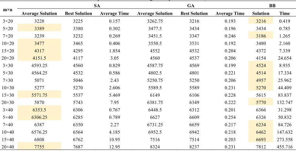
TABLE 5. Computational results for large scale problems for SA,GA and BB
m×n
SA GA BB
Average Solution Best Solution Average Time Average Solution Best Solution Average Time Solution Time
3×20 3228 3225 0.157 3262.75 3216 0.193 3216 0.419
5×20 3389 3380 0.302 3477.5 3434 0.196 3434 0.785
7×20 3239 3232 0.269 3451.5 3347 0.246 3186 1.265
10×20 3477 3465 0.406 3550.5 3531 0.192 3480 2.160
15×20 4317 4295 1.854 4552 4532 0.204 4372 7.339
20×20 4151.5 4117 3.05 4560 4537 0.206 4154 24.654
3×30 4593.25 4560 0.829 4587.75 4569 0.199 4524 8.935
5×30 4564.25 4532 0.586 4802.5 4801 0.221 4514 17.334
7×30 5071 5046 2.43 5250.75 5250 0.206 4957 25.962
10×30 5277 5270 2.606 5589.5 5589 0.231 5270 44.409
15×30 5571.75 5537 5.469 6149 6106 0.228 5615 83.837
20×30 5870 5743 7.95 6381.75 6349 0.222 5770 132.747
3×40 6353.5 6306 0.767 6448.5 6312 0.201 6366 31.298
5×40 6306.25 6285 0.789 6627 6609 0.254 6326 50.832
7×40 6387 6350 2.27 6731.25 6659 0.217 6234 84.726
10×40 6576.25 6564 4.185 6952.5 6942 0.218 6462 147.632
15×40 6808 6762 10.95 7516 7514 0.203 6693 273.558
20×40 7755 7687 12.95 8324 8237 0.231 7812 455.716
TABLE 6.Computational results for small scale (1)
Number of optimal solutions
Number of better solution than GAMS
Average error of methods compared to
GAMS Average computational time (s)
SA GA BB SA GA BB SA GA BB SA GA GAMS BB
16
Figure 3.Time series plot for proposed algorithms in small scale
Figure 4.Time series plot for computational time in small
scale
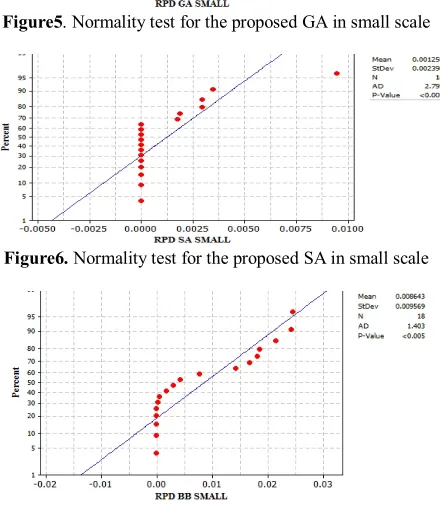
Figure5. Normality test for the proposed GA in small scale
Figure6. Normality test for the proposed SA in small scale
Figure7. Normality test for the proposed BB in small scale
Figure8. Results of Kruskal-Wallis test for small scale
TABLE 7.Computational results for small scale (2)
Method Objective function average value
GAMS 1305.833
SA 1308.139
GA 1322.236
BB 1317.389
As it can be seen from Figure8, as well as the P=0.961, the p-value is above 0.05.So, we can declare that the result is not statistically significant, or there is not a statistically significant difference between the algorithms.
6. 2. Analyzing Large Scale Problems
Considering Figure 9, we can see that in the large scale problems, SA and BB are very close to each other in most cases and both excel GA algorithm clearly. Totally, the proposed BB outperforms the GA and SA algorithms in large scale problems considering the objective function value. In Figure10, it can be seen that in most cases, the time taken to reach optimal solution in proposed GA is less than the proposed SA and BB algorithms. This leads the proposed BB to be more efficient in solving the large scale problems due to the computation time.
TABLE 8.Computational results for large scale (1)
Method Objective function average value Computational time average value
SA 5163.042 3.2121
GA 5450.819 0.2148
BB 5132.5 77.422
TABLE 9. Computational results for large scale (2)
Average error of GA compared to
SA
Average error of GA compared to
BB
Average error of SA compared to BB
0.936 1.042 0.100
Figure 9. Changes in the objective function of the proposed
algorithms in large scale
Figure 10. Changes of computation times in order to achieve
the optimal solutions of the proposed algorithms in large scale
Figure 11. Normality test for GA in large scale
Figure 12. Normality test for SA algorithm in large scale
Figure 13. Normality test for BB algorithm in large scale
Figure 14. Results of Kruskal-Wallis test for large scale
6. CONCLUSIONS
This paper dealt with the no-wait reentrant flowshop scheduling problem to minimize makespan. Since this problem has been proved to be NP-hard, heuristic algorithms were proposed in this paper to solve it. To our best knowledge, this should be the first proposed model for the problem with the above-mentioned properties. Computational results show that, considering both small scale and large scale, SA algorithm outperforms the two other algorithms in finding better solutions in a proper computational time.
A perspective for future research is to develop other metaheuristics for the model and compare the results with the proposed algorithms. In the real world, the nature of variables is not deterministic, so the fuzzy approach can be applied to the problem. Finally, generalizing the model to other layouts such as flexible flowshop can be an interesting path for future work.
7. REFERENCES
1. Aldowaisan, T., & Allahverdi, A.,"New heuristics for no-wait flowshops to minimize makespan",Computers & Operations Research, Vol.30, No.8 , (2003), 1219-1231 .
2. Attar, S., Mohammadi, M., & Tavakkoli-Moghaddam, R.,"A novel imperialist competitive algorithm to solve flexible flow shop scheduling problem in order to minimize maximum completion time",International Journal of Computer Applications, Vol.28, No,10,(2011), 27-32 .
3. Chen, C.-L., & Chen, C.-L.,"A bottleneck-based heuristic for minimizing makespan in a flexible flow line with unrelated parallel machines",Computers & Operations Research, Vol.36, No.11, (2009), 3073-3081.
Journal of Advanced Manufacturing Technology, Vol.29, No.11, (2006), 1186-1193 .
5. Dugardin, F., Yalaoui, F., & Amodeo, L.,"New multi-objective method to solve reentrant hybrid flow shop scheduling problem",European Journal of Operational Research,Vol.203, No.1, (2010), 22-31 .
6. Emmons, H., & Vairaktarakis, G.,"Flow shop scheduling: theoretical results, algorithms, and applications",Springer Science & Business Media,Vol. 182,(2012).
7. Graham, R. L., Lawler, E. L., Lenstra, J. K., & Kan, A. R.,"Optimization and approximation in deterministic sequencing and scheduling: a survey",Annals of Discrete Mathematics,
Vol.5,(1979), 287-326 .
8. Gupta, J. N., Strusevich, V. A., & Zwaneveld, C. M.,"Two-stage no-wait scheduling models with setup and removal times separated",Computers & Operations Research, Vol.24, No.11, (1997), 1025-31.
9. Hall, N. G., & Sriskandarajah, C.,"A survey of machine scheduling problems with blocking and no-wait in process",Operations Research,Vol.44, No.3,(1996), 510-525 . 10. Hsieh, B.-W., Chen, C.-H., & Chang, S.-C.,"Efficient
simulation-based composition of scheduling policies by integrating ordinal optimization with design of experiment",Automation Science and Engineering, IEEE Transactions on, Vol.4, No.4,(2007), 553-568 .
11. Huang, R.-H., Yu, S.-C., & Kuo, C.-W.,"Reentrant two-stage
multiprocessor flow shop scheduling with due windows",The International Journal of Advanced Manufacturing Technology, Vol.71,(2014), 1263-1276 .
12. Jing, C., Huang, W., & Tang, G.,"Minimizing total completion time for re-entrant flow shop scheduling problems",Theoretical Computer Science, Vol.412, No.48, (2011), 6712-6719 . 13. McCormick, S. T., & Rao, U. S.,"Some complexity results in
cyclic scheduling". Mathematical and Computer Modelling,
Vol.20, No.2, (1994), 107-122 .
14. Pan, J. C.-H., & Chen, J.-S.,"Mixed binary integer programming formulations for the reentrant job shop scheduling problem",Computers & Operations Research,Vol.32, No.5, (2005), 1197-1212 .
15. Qian, B., Wan, J., Liu, B., Hu, R., & Che, G.-L.,"A DE-based algorithm for reentrant permutation flow-shop scheduling with different job reentrant times", Paper presented at the Computational Intelligence in Scheduling (SCIS), (2013). 16. Shafaei, R., Rabiee, M., & Mirzaeyan, M.,"An adaptive neuro
fuzzy inference system for makespan estimation in multiprocessor no-wait two stage flow shop",International Journal of Computer Integrated Manufacturing,Vol.24, No.10,(2011), 888-899 .
17. Yang, D.-L., Kuo, W.-H., & Chern, M.-S., "Multi-family scheduling in a two-machine reentrant flow shop with setups".
European Journal of Operational Research,Vol.187, No.3,
(2008), 1160-1170.
Solving Re-entrant No-wait Flowshop Scheduling Problem
S. Tasouji Hassanpour, M. R. Amin-Naseri, N. Nahavandi
Department of Industrial Engineering, Tarbiat Modares University, Iran
P A P E R I N F O
Paper history:
Received 29December 2014
Received in revised form 16February 2015 Accepted 11 June 2015
Keywords: Re-entrant Flowshop No-wait Flowshop Genetic Algorithm Simulated Annealing Bottleneck ﺪﯿﮑﭼ ه ارد ﯾ ﻦ نﺎﻣزﻪﻟﺎﻘﻣ ﺪﻨﺑ ي ﺮﺟﻪﻟﺎﺴﻣ ﯾ نﺎ ﻫﺎﮔرﺎﮐ تﺎﯿﺻﻮﺼﺧﻦﺘﻓﺮﮔﺮﻈﻧردﺎﺑﯽ ﺖﺸﮔﺮﺑ ﯾﺬﭘ ﺮ و ﻪﻔﻗونوﺪﺑ ﻂﯿﺤﻣندﻮﺑ فﺪﻫﺎﺑ ﻤﮐ ﯿ ﻪﻨ يزﺎﺳ ﻤﮑﺗنﺎﻣزﺮﺜﮐاﺪﺣ ﯿ ﻞ ﺳرﺮﺑﺎﻫرﺎﮐ ﯽ ﻣ ﯽ دﻮﺷ .
ﺖﺸﮔﺮﺑﻂﯿﺤﻣﯽﻠﺻاﯽﮔﮋﯾو ﻪﮐﺖﺳاﻦﯾاﺮﯾﺬﭘ
ﻞﻗاﺪﺣنآرد ﯾ ﮏ ﻣرﺎﮐ ﯽ ﯾﺎﺑ ﺴ ﺖ زا ﯾ ﮑ ﯿﺎ ﺑﻪﻠﺣﺮﻣﺪﻨﭼ ﯿ ﺶ زا ﯾ رﺎﺒﮑ درﺬﮕﺑ .
ﻪﻔﻗونوﺪﺑﯽﻫﺎﮔرﺎﮐنﺎﯾﺮﺟﻞﯾﺎﺴﻣرد يورﺮﺑيرﺎﮐشزادﺮﭘﯽﺘﻗو،
ﯽﻣعوﺮﺷلواﻦﯿﺷﺎﻣ ،دﻮﺷ
ﺪﯾﺎﺑ ﻪﻔﻗوﻪﮑﻨﯾانوﺪﺑ ﺑنآرديا
ﻪ ﺪﯾآدﻮﺟو ، يورتﺎﯿﻠﻤﻋ مﺎﻤﺗاﺎﺗاردﻮﺧﯽﺷزادﺮﭘﺮﯿﺴﻣ
ﯽﻃﺮﺧآﻦﯿﺷﺎﻣ ﺪﻨﮐ . ودﺮﻫمﺎﻏدا ي اﯾ ﻦ ﺻﻮﺼﺧ ﯿ تﺎ ﺴﺑرد ﯿ رﺎ ي ﺎﻨﺻزا ﯾﻊ ﺎﻨﺻﺪﻨﻧﺎﻣ ﯾﻊ ﺗﺎﺑر ﯿ ﮏ ﺑداردﻪﮐدراددﺮﺑرﺎﮐ ﯿ
تﺎ ﺑ ﻪ
ﺳرﺮﺑاﺰﺠﻣترﻮﺻ ﯿ ﻫﺪﺸﻨ ﺖﺳﺎ . اﺪﺘﺑا اﺮﺑ ي ﻪﻟﺎﺴﻣ ﮏﯾﺮﻈﻧﺪﻣ رلﺪﻣ ﯾ ﺿﺎ ﯽ ارا ﯾﻬ يدﺎﻬﻨﺸﯿﭘشورﻪﺳزاهدﺎﻔﺘﺳاﺎﺑﺲﭙﺳﻮ
ﻠﺣ هﺪﺸ ﺖﺳا
.
ﻢﺘﯾرﻮﮕﻟا ﺎﮔﻮﻠﮔﺮﺑﯽﻨﺘﺒﻣﻢﺘﯾرﻮﮕﻟاﮏﯾوﮏﯿﺘﻧژﻢﺘﯾرﻮﮕﻟا،ﺪﯾﺮﺒﺗيزﺎﺳﻪﯿﺒﺷﻞﻣﺎﺷيدﺎﻬﻨﺸﯿﭘيﺎﻫ ﯽﻣه
ﺪﺷﺎﺑ
.
رد
شورﯽﯾآرﺎﮐ،ﺖﯾﺎﻬﻧ ﯽﺳرﺮﺑوﯽﺑﺎﯾزراهﺪﺷﻪﯾارايﺎﻫ
هﺪﺷ ﺖﺳا
.