Numerical Solution of Optimal Control of Time-varying Singular Systems via Operational Matrices

(1)

International Journal of Engineering

J o u r n a l H o m e p a g e : w w w . i j e . i r

Numerical Solution of Optimal Control of Time-varying Singular Systems via

Operational Matrices

M. Behroozifara_{, S. A. Yousefi}b_{, A. Ranjbar N.}c*

a_{Faculty of Basic Sciences, Babol University of Technology, Babol, Iran} b_{Department of Mathematics , Shahid Beheshti University, Tehran, Iran}

c_{Faculty of Electrical Engineering, Department of Control and Instrumentation, Babol University of Technology, Babol, Iran}

P A P E R I N F O

Paper history:

Received 17 April 2013

Accepted in revised form 22 August 2013

Keywords: Optimal Control Time-varying Singular Systems Operational Matrices Kronecker Product Bernstein Polynomial

A B S T R A C T

In this paper, a numerical method for solving the constrained optimal control of time-varying singular systems with quadratic performance index is presented. Presented method is based on Bernstein polynomials. Operational matrices of integration, differentiation and product are introduced and utilized to reduce the solution of optimal control problems with time-varying singular systems to the solution of algebraic equations set. The strength of the method is shown by exhibiting a numerical implementation using operational matrices that solves the determined control problem by solving an equation set. The method converges rapidly to the exact solution and gives very accurate results even

by low value of . Illustrative examples are included to demonstrate the validity and efficiency of the

technique and convergence of method to the exact solution especially for unstable singular systems.

doi:10.5829/idosi.ije.2014.27.04a.03

1. INTRODUCTION1

Problem of optimal control of singular systems is an immense interest; especially those researchers are investigating on the existing problems in the field of control theory and in numerical computation of the value of control vector which is controlling the state vector. These types of systems are encountered in many areas, such as network theory, economics, demography, neural systems, composite systems, etc. Chen and Hsiao [1] and Chen and Shih [2] have used Walsh series to study the problem of optimal control of time-invariant and time-varying linear systems. A review of the literature suggests that Cobb [3] and Pandolfi [4] were the first authors to consider the optimal regulator problem of continuous-time singular systems. Both the used state feedback and the results were derived with the aid of Ricatti-type matrix equations. Walsh functions have been widely used to study problem of optimal control of linear systems with quadratic

*_{Corresponding Author Email:}_{[email protected] (A. Ranjbar N.)}

(2)

Davison [17] constitute a representative collection of the other works. Recently, a numerical algorithm to obtain the consistent conditions satisfied by singular arcs for singular linear-quadratic(LQ) optimal control problems is presented in [18]. In [19] the existence of singular arcs for optimal control problems is studied by using a geometric recursive algorithm inspired in Dirac’s theory of constraints. For more information on the mathematical modeling and solution of this model and some other similar models, we refer the interested reader to the papers [20-30]. [19, 20] [21-30]

In this paper, Bernstein polynomial basis is used for solving an optimal control of time-varying singular system with a quadratic cost function. In the following, major difficulties and challenges which are to be met in the paper are summarized. At first, state vector ̇( ) and control vector ₍ ₎ are expanded in terms of Bernstein polynomial. Operational matrices of Bernstein polynomial are applied to estimate ₍ ₎ using _̇₍ ₎. In section 6, when _≤ by a technic the system dynamics and cost function (performance index) are approximated, then a new minimization problem is attained. Approximated solution of problem is calculated using the Lagrange multipliers method. These unknown coefficients are determined in such a way that the necessary conditions for extremization are met. The presented method shows that a more accurate solution of the time-varying optimal control of linear singular systems with a quadratic performance index can be obtained. Numerical evidence of the stability of the algorithm will be presented by discussing various relevant numerical experiments.

This paper is structured as follows: in section 2, problem of time-varying singular system is described. Section 3 describes the basic formulation of Bernstein polynomials which is required for our subsequent development. Section 4 is devoted to the function approximation using Bernstein polynomial basis whilst the upper bound of approximation error is deduced. In section 5, we elaborate operational matrices of integration, differentiation, dual and product using Kronecker product [31]. In section 6, solution of time-varying singular system problem is approximated by Bernstein polynomial basis and an algebraic equation set is presented using Lagrange multipliers method. In section 7, numerical findings are presented which demonstrate the validity, accuracy and applicability of our new method. Section 8 consists of the remark and brief summary.

2. STATEMENT OF THE PROBLEM

Consider following time-varying singular system: () ̇() = () ( ) + ( ) ( ),

( ) = , (1)

where the matrix ( ) is singular, ( )∈R is a generalized state vector, ( )∈R is a control vector, ( ) and ( ) are known coefficient matrices associated with ( ) and ( ) with appropriate dimensions, respectively, and is the given initial state vector.

In order to minimize a cost function, considering both state and control signals of the feedback control system, a quadratic performance index is usually minimized:

= ( ) ( ) + ∫ [ () ( ) ()

+ () ( ) ()] ,

(2)

where and are prescribed times, ∈R × _and

( ) are weighting matrices for ( ) and is a symmetric and positive definite (or semi definite) matrix, ( ) is a weighting matrix for ( ), ( ) and ( ) are matrices with appropriate dimensions [32].

3. PROPERTIES OF BERNSTEIN POLYNOMIALS

Bernstein polynomials of _{degree are defined on}

[ , ] as [5, 6, 7, 23]:

, ( ) = ( )( )( )

( ) , 0≤ ≤

where

( ) = _!(! _)!.

These Bernstein polynomials form a basis on [a,b]. There are m + 1 number _{degree polynomials. For}

convenience, , ( ) = 0, if < 0 or > . A

recursive definition can also be used to generate the Bernstein polynomials over _{[ ,}_] as:

, ( ) =( ) , ( ) + , ( ).

It can be shown that each of the Bernstein polynomials are positive and linear independent and the sum of all the Bernstein polynomials is unity for all real ∈[ , ], i.e., ∑ , ( ) = 1. It is easy to show that any given

polynomial of degree can be expanded in terms of these basis functions.

4. APPROXIMATION OF FUNCTIONS

Suppose that = [ , ] where , ∈R , let { , , , ,⋯, , }⊂ is the set of Bernstein

polynomials of _{degree and}

= { , , , ,⋯, , }

and is an arbitrary element in . Since is a finite dimensional vector space, has a unique best approximation out of , say ∈ , that is:

(3)

where || || = < , > and < , >=∫ () () . In [39], it is shown that a unique coefficient vector

= [ , ,⋯, ] exists such that:

≈ =∑ , = ϕ, (3)

where ϕ = [ , , , ,⋯, , ] and can be

obtained:

= ∫ ( )ϕ( ) _, ₍₄₎

which is said dual matrix of ϕ and introduced as: =< , >=∫ ϕ( )ϕ( ) .

Theorem 1. Suppose that be a Hilbert space and be a closed subspace of such that <∞ and { , ,⋯, } is any basis for . Let be an arbitrary element in and be the unique best approximation to out of . Then

|| − || = (₍, _,, _,_⋯,⋯_,, ₎), where

( , , ,⋯, ) =

< , > < , > ⋯ < , > < , > < , > ⋯ < , > ⋮ ⋮ ⋮ ⋮ < , > < , > ⋯ < , >

.

Proof. [33].

Exact value of approximation error is presented by the Theorem 1. In the following lemma, an upper bound of approximation error is presented.

Lemma 1. Suppose that function : [ , ]→ be + 1 times continuously differentiable, ∈ _[ _, _],_and ₌_{

, , , ,⋯, , }. If

ϕ be the best approximation out of then the mean error bound is presented as follows:

|| − ϕ|| ≤ ( − )

( + 1)!√2 + 3 , where = max ∈[ , ]| ( )( )|.

Proof. [34].

Lemma 1 shows that the method of approximation converges to when →∞.

Now, let ( ) = [ ( ), ( ), . . . , ( )] where ( )∈ for = 1, 2, . . . , . If we approximate ( ) out of by (3), we have:

( )≈ ϕ

where _{= [}_, _, _, _{, . . . ,} _, _] can be calculated by (4) for = 1,2, . . . , . Then

= _⋮ ≈ ⎣ ⎢ ⎢ ⎡ ϕ

ϕ ⋮ ϕ⎦⎥

⎥ ⎤ = , , , ⋮ , + , , , ⋮ , +⋯+ , , , ⋮ ,

= , , , , … , , =ϕ , where is the identity matrix of order ,

= [ , , , , . . . , , , , , , , . . . , , , . . . , , , , , . . . , , ]

is a matrix 1 × [ ( + 1)] and

ϕ = , , ⋮

,

=ϕ⊗ , (5)

where _⊗ denotes the Kronecker product [31], so

= ϕ . (6)

We can also approximate a matrix of functions using (6). Therefore, suppose that _× ( ) = [ , ( )] × =

( ) ( ) ⋮

( )

where _, ( )∈ and ( ) is _{row of}_{( )}

for = 1,2, . . . , .

If we approximate ( ) out of by (6), we will get ( )≈ ( )ϕ ( ) for = 1,2, . . . , , then

= _⋮ ≈

⎣ ⎢ ⎢ ⎢ ⎡ ϕ

ϕ ⋮ ϕ⎦⎥

⎥ ⎥ ⎤ = ⎣ ⎢ ⎢ ⎢ ⎡ ⋮ ⎦⎥ ⎥ ⎥ ⎤

ϕ = ϕ (7)

where ×[ ( )]=

⎣ ⎢ ⎢ ⎢ ⎡ ⋮ ⎦⎥ ⎥ ⎥ ⎤ .

5. OPERATIONAL MATRICES

Operational matrices of the integration , differentiation dual and product of vector ϕ are respectively defined by:

∫ ϕ() ≈ ϕ( ), ≤ ≤

( )

≈ ϕ( ),

=∫ ϕ( )ϕ ( ) ,

ϕ( )ϕ( ) ≈ϕ( ) ,

(4)

Analogously, we can define [ ( + 1)] × [ ( + 1)] operational matrices of _ϕ as:

∫ ϕ () ≈Pϕ ( ), ≤ ≤ ,

( )

≈D ϕ ( ) ,

ϕ =∫ ϕ ( )ϕ ( ) ,

ϕ ( )ϕ ( ) ≈ϕ ( ) ,

which is an arbitrary × [ ( + 1)] matrix.

It can be easily shown that the operational matrices of the integration, differentiation and dual of ϕ are as:

= ⊗ ,

= ⊗ .

(8)

5. 1. Operational Matrix of Product of It is aimed to derive an explicit formula for operational matrix of product of ϕ . Suppose that = [ , , . . . , ] is an arbitrary × [ ( + 1)] matrix where is × matrix for = 0,1,2, . . . , , then is [ ( + 1)] × [ ( + 1)] operational matrix of product of _ϕ whenever

ϕ ( )ϕ ( ) ≈ϕ ( ) .

Since _ϕ ₍ _{) =}∑ , ( ), we have

ϕ ( )ϕ ( ) =

∑ _, ( ) _, ( ),∑ _, ( ) , ( ), ⋯,

∑ , ( ) , ( )].

Now, we approximate all functions _, ( ) , ( ) in

terms of { , ( )} for , = 0,1,⋯, , i.e, we must

find vector _, = [ ,, ,, ,, … , ,] by (4) such that

, ( ) , ( )≈ ,ϕ( ), , = 0,1,⋯, .

Therefore, for = 0,1,⋯,

∑ , ( ) , ( )≈∑ ∑ , , ( )

=∑ , ( ) ∑ , =ϕ ( ) ⎣ ⎢ ⎢ ⎢

⎡∑ , ∑ , ⋮ ∑ ,_⎦⎥

⎥ ⎥ ⎤

=ϕ ( ) , ⊗ , , ⊗ , ⋯, , ⊗ _⋮ =

ϕ ( )

where

= , ⊗ , , ⊗ , ⋯, , ⊗ _⋮ .

If we define [ ( + 1)] × [ ( + 1)] matrix =

, ,⋯, , then

ϕ ( )ϕ ( )

= ∑ , ( ) , ( ),∑ , ( ) , ( ), ⋯,

∑ , ( ) , ( )]

≈ϕ ( ) , , ⋯, =ϕ ( ) ,

therefore

ϕ ( )ϕ ( ) ≈ϕ ( ) . (9) so is the operational matrix of product of ϕ .

6. SOLUTION OF PROBLEM USING BERNSTEIN POLYNOMIALS BASIS

6. 1. Approximation of the System Dynamics We approximate (1) as follows:

Let ≤ ( for ≥ follows quite same) and

̇() = [ ̇ (), ̇ (), . . . , ̇ ()] , (10)

() = [ (), (), . . . , ()] . (11) Using (3), each of ̇ ( ) and each of ( ), = 1, 2, . . . , , = 1, 2, . . . , , can be approximated in terms of basic functions as ̇ ( ) = ϕ( ) and ( ) = ϕ( ) where _{= [} _, _, _, _{, . . . ,} _, _] and ₌ [ , , , , . . . , , ] which can be calculated by (4).

Then we can write (10), (11) by (6) as:

̇() =ϕ () (12)

() =ϕ () (13)

where

= [ , , , , . . . , , , , , , , . . . , , , . . ., , , , , . . . , , ],

and

= [ , , , , . . . , , , , , , , . . . , , ,

. . . , , , , , . . . , , ]. (14) From (10) and (8) we have:

() =ϕ () + ( ) =ϕ () (15)

where = + and ( ) =ϕ ( ) . Now, we approximate matrices and by (7)

≈ ϕ , (16)

≈ ϕ , (17)

since ≤ ,

(5)

where ∗_{= [} _, _{, . . . ,} _]_, ∗_{= [} _, _{, . . . ,} _] _in

which ₌

0 0 ⋮ 0

and _{= 0} for ₌ _{+ 1,} _{+ 2, . . . ,} _.

If we approximate ∗_and ∗_{by (7) and (6),} respectively, we get:

∗_≈∗_ϕ_,

∗_≈_ϕ ∗_,

where

∗_{= [}

, , , , . . . , , , , , , , . . . , , , . . . , , , , , . . . , , ] ,

therefore

= ∗ ∗_≈∗_ϕ _ϕ ∗_. (18)

Substituting (12), (15), (16), (17) and (18) in (1) we obtain:

Eϕ ϕ = ϕ ϕ + ∗_ϕ_ϕ ∗_, (19) using (9) we have:

ϕ ϕ ≈ϕ , (20)

∗_ϕ _ϕ _≈_ϕ ∗_, (21)

ϕ ϕ ≈ϕ , (22)

where , ∗_and _{are operational matrices of} product, by replacing (20), (21) and (22) in (19) we get ϕ =ϕ X+ϕ ∗∗_,

so

X+ ∗∗₋ _{= 0.} ₍₂₃₎

6.2. The Performance Index Approximation Now, we approximate (2) as follows:

At first, we approximate matrices and by (7), i.e.

≈ ϕ , (24)

≈ ϕ . (25)

Substituting (13), (15), (24) and (25) in (2) we obtain:

= ( ) ( ) + ∫ [ () () () + () () ()] ≈ ϕ ( ) ϕ ( ) + ∫ [ ϕ () ()ϕ ()ϕ ()

+ ϕ () ()ϕ ()ϕ () ] ,

(26)

by using (9) we have:

()ϕ ( ) ϕ () ≈ϕ () , (27)

( )ϕ ( ) ϕ ( ) ≈ϕ ( ) , (28)

which and are operational matrices of product. By replacing (27) and (28) in (26), and using (8) we get:

≈ ϕ ϕ

+ + . (29)

6. 3. Solution of the Optimization Problem From (23) and (29) in sections (6.1) and (6.2), respectively, the main problem is reduced to:

ϕ ϕ + [ + ]

:

+ ∗₋ _{= 0.}

Using the Lagrange multipliers method, Lagrangian equation for this problem is:

∗₌ _ϕ _ϕ ₊ ₊ ]+λ [ + ∗₋ _],

therefore, unknown coefficients cab be calculated by solving the following system of algebraic equations:

∗

= 0,

∗

= 0,

∗ = 0.

Unknown coefficients can be found by simultaneously solving the above system of algebraic equations (e.g. using ℎ _).

7. ILLUSTRATIVE EXAMPLES

In order to show the performance of the presented method in this paper we applied it to solve some examples. The following case studies are given to show the merit of the proposed method. This method differs from other methods presented in [9, 10, 23, 35] and thus could be used as a basis for comparison.

Example 1. Consider the optimal control of time-varying singular system presented in [10]:

1 0

− 0 ̇̇ (()) = 1 +−1 0 −1 () + 01 ( ), 0≤ ≤2,

(0) = 1,

with the optimal control minimizing the performance index

= ∫ ( + ) ,

whose exact solutions under the above-mentioned constraints is:

() = _,

(6)

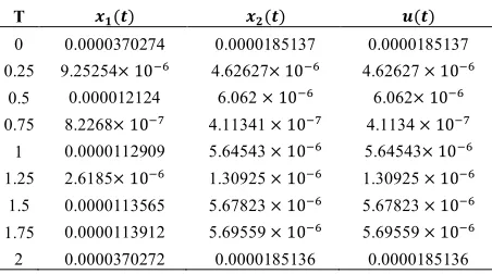
Here, we solve the problem using Bernstein polynomials of degree = 5, 10 and present the absolute error of ( ), ( ) and ( ) on some points in Table 1 and Table 2, respectively. In Figures 1 and 2 images of exact and estimated solutions of ( ), ( ) and ₍ ₎ for _{= 10} are ploted, respectively.

The exact value of optimal control and estimated values of optimal control by = 5, 10 are equal to = 0.36813163541672467 and _.= 0.3681316353957 and _.= 0.368131635789, respectively. This example shows that absolute error decreases rapidly when degree of Bernstein polynomials are doubled.

Note that, the given exact solutions in [10]

() = _, ₍_{) =} _{+ sin}_, ₍_{) = sin}

with initial points (0) = 1₁ is failed to meet the optimality requirement because the value of optimum control is = 2.14667246697579 by the presented exact solutions in [30] whereas there are some solutions which satisfy on given constraints with lower optimal control value, for example:

() = _, ₍_{) =} ₊ _, ₍_{) =}

provide the optimum control value

.= 1.4545059223673806. Likewise

( ) = _, ₍ _{) =} ₊

, ( ) =

provide the optimum control value

.= 0.49704878872520114 or () = _,

() = ₊

, ( ) =

the optimum control value _.= 0.4913621261074325 and etc. In fact, using Euler-Lagrange equation it can be demonstrated that this problem does not have an optimum solution with initial points (0) = 1₁, so we

have to change the initial points to (0) = 1 and then solve it analytically using Euler-Lagrange equation to obtain exact solutions.

TABLE 1. The absolute error of ₍₎, ₍ ₎ and ₍ ₎ with

m=5 for example 1.

T ( ) ₍ ₎ ₍ ₎

0 0.0000370274 0.0000185137 0.0000185137

0.25 9.25254×10 _4.62627_{× 10} _4.62627_{× 10}

0.5 0.000012124 6.062 _×₁₀ _6.062_{× 10}

0.75 8.2268×10 _4.11341_×₁₀ _4.1134_{× 10}

1 0.0000112909 5.64543 ×10 _5.64543_{× 10}

1.25 2.6185_×₁₀ _1.30925_×₁₀ _1.30925_{× 10}

1.5 0.0000113565 5.67823 ×10 _5.67823_{× 10}

1.75 0.0000113912 5.69559 _×₁₀ _5.69559_{× 10}

2 0.0000370272 0.0000185136 0.0000185136

Figure 1. Exact and estimated solutions for () with = 10 in example 1.

Example 2. Consider the optimal control of unstable

time-varying singular system 2 0

0 ̇̇ (()) = −4 0 1 ( ) + 02 (), 0≤ ≤2,

(7)

and the performance index = ∫ ( + ) .

The objective is to determine an optimal control u(t) that will drive from an admissible initial state (0−) =

to some desired final state in a given time and minimize the above cost function (performance index). The exact solution for = 2 is:

() = _, ₍_{) =} _, ₍_{) =} _.

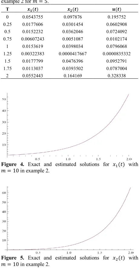
The absolute error of ( ), ( ) and corresponding optimal control u (t) are calculated in some points using Bernstein polynomials of degree = 5, 10 and the results are presented in Table 3 and Table 4, respectively. In Figures 3, 4 and 5 images of exact and estimated solutions of ( ), ( ) and ( ) for = 10 are ploted, respectively. The exact value of optimal control and estimated values of optimal control by = 5, 10 are equal = 2468.4527080 and _. _{= 2468.36}, _._{= 2468.452638},

respectively. From numerical results, it can be found that the method provides high efficiency and uniformly converges to the exact solution and gives accurate solutions especially for unstable singular systems. Also, this example shows that absolute error decreases rapidly when degree of Bernstein polynomials are doubled.

Example 3. Consider the optimal control of singular

system presented in [9, 23, 35]: 0 1

0 0 ̇̇ (()) = 1 00 1 ( )+ 01 (), 0≤ ≤2,

(0) = 1₋√ ,

by minimizing the performance index = ∫ ( + ) ,

whose exact solutions under the above-mentioned constrains is:

() = √ _,

() =−√ √ _, ₍_{) =}√ √ _.

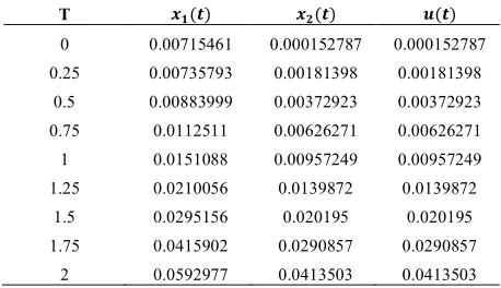
We approximate ( ), ( ) and ( ) by Bernstein polynomials of degree _{= 3, 5, 7} on interval _{[0, 2]} and present the absolute error of ( ), ( ) and ( ) for some points in Table 5, Table 6 and Table 7, respectively. The exact value of optimal control and estimated values of optimal control by = 3, 5, 7 are equal = 0.35231825561 ,_.= 0.351089, .= 0.351092 and .= 0.351092, respectively. Numerical results demonstrate the feasibility of the method.

TABLE 2. The absolute error of x₁(t), x₂(t) and u(t) with

m=10 for example 1.

T ₍₎ ₍₎ ₍ ₎

0 2.74002´₁₀-11 1.15576´ ₁₀-11 _1.49232´₁₀-11

0.25 2.20091´ ₁₀-12 9.27175´₁₀-12 1.10639´₁₀-12

0.5 2.23621´₁₀-12 2.67986´ ₁₀-11 7.24032´ ₁₀-13

0.75 2.03171´ ₁₀-12 _3.66686´₁₀-10 _8.26469´₁₀-12

1 5.57443´ ₁₀-13 _1.37799´₁₀-9 _2.19486´₁₀-11

1.25 9.66172´ ₁₀-13 2.55455´ ₁₀-9 2.9886´ ₁₀-11

1.5 1.23643´ ₁₀-12 3.33117´ ₁₀-9 _2.32852´₁₀-11

1.75 3.0749´₁₀-12 _3.5851´₁₀-9 _6.61682´₁₀-12

2 2.74002´ 11

10- _3.59851´ ₁₀-9 1.371´ ₁₀-11

TABLE 3. The absolute error of (), () and () of example 2 for _{= 5}.

T ₍₎ ₍₎ ₍₎

0 0.0543755 0.097876 0.195752

0.25 0.0177606 0.0301454 0.0602908

0.5 0.0152232 0.0362046 0.0724092

0.75 0.00607243 0.0051087 0.0102174

1 0.0153619 0.0398034 0.0796068

1.25 0.00322383 0.0000417667 0.0000835332

1.5 0.0177799 0.0476396 0.0952791

1.75 0.0113037 0.0393502 0.0787004

2 0.0552443 0.164169 0.328338

(8)

TABLE 4. The absolute error of (), ( ) and () of example 2 for = 10.

T () () ()

0 1.21003×10 _3.99602_×₁₀ _7.9868_×₁₀

0.25 1.54127_×₁₀ _1.93468_×₁₀ _8.00346_×₁₀

0.5 3.1485_×₁₀ _8.06245_×₁₀ _4.75277_×₁₀

0.75 1.85167×10 _2.71612_×₁₀ _5.2744_×₁₀

1 4.81083×10 _3.63834_×₁₀ _9.99076_×₁₀

1.25 1.10634×10 _3.27331_×₁₀ _6.04075_×₁₀

1.5 1.18365×10 _3.36985_×₁₀ _7.09836_×₁₀

1.75 7.77893×10 _3.20602_×₁₀ _9.26404_×₁₀

2 1.21003×10 _8.01143_×₁₀ _0.00001089

TABLE 5. The absolute error of ( ), ( ) and ( ) of example 3 for = 3.

T ₍₎ ₍₎ ₍₎

0 0.0169508 0.00794424 0.00794424

0.25 0.00350157 0.00478137 0.00478137

0.5 0.00689598 0.00542015 0.00542015

0.75 0.0137541 0.0044623 0.0044623

1 0.0185624 0.0068358 0.0068358

1.25 0.0213305 0.0135629 0.0135629

1.5 0.0259471 0.0229231 0.0229231

1.75 0.0390242 0.0312704 0.0312704

2 0.0690859 0.0336063 0.0336063

TABLE 6. The absolute error of ( ), ( ) and ( ) of example 3 for = 5.

T () () ()

0 0.00715461 0.000152787 0.000152787

0.25 0.00735793 0.00181398 0.00181398

0.5 0.00883999 0.00372923 0.00372923

0.75 0.0112511 0.00626271 0.00626271

1 0.0151088 0.00957249 0.00957249

1.25 0.0210056 0.0139872 0.0139872

1.5 0.0295156 0.020195 0.020195

1.75 0.0415902 0.0290857 0.0290857

2 0.0592977 0.0413503 0.0413503

TABLE 7. The absolute error of ( ), ( ) and ( ) of example 3 for _{= 7}.

T () () ()

0 0.00696458 1.53036_{× 10} _1.53036_{× 10}

0.25 0.00740281 0.00177682 0.00177682

0.5 0.00877684 0.00377894 0.00377894

0.75 0.0112602 0.00625787 0.00625787

1 0.0151665 0.00952659 0.00952659

1.25 0.0209867 0.0139999 0.0139999

1.5 0.029459 0.0202406 0.0202406

1.75 0.0416522 0.0290377 0.0290377

2 0.0591077 0.0415015 0.0415015

8. CONCLUSION

In the present work, a technique has been developed for obtaining an optimal control of time-varying singular systems with a quadratic cost function using Bernstein polynomials. The operational matrices of integration, differentiation and product of Bernstein polynomials basis are introduced and are utilized to reduce the optimal control of time-varying singular system to the solution of algebraic equations. The proposed method is general, easy to implement, and yields accurate results. Absolute error reduced quickly when degree of Bernstein polynomials is increased, but when ≥15, volume of computations increases and obtained algebraic equation set is difficultly solved which is one of the limitation of this method. Simulation results give a satisfactory solution and demonstrate good performance of the proposed methods for solving optimal control of time-varying singular systems. Numerical tests also show that the method converges to the exact solution and can be used for unstable singular systems.

9. ACKNOWLEDGMENT

Authors are very grateful to both reviewers for carefully reading the paper and for their helpful comments and suggestions which have improved the paper.

10. REFERENCES

1. Chen, C. and Hsiao, C., "Walsh series analysis in optimal control", International Journal of Control, Vol. 21, No. 6, (1975), 881-897.

2. Chen, W.-L. and Shih, Y.-P., "Analysis and optimal control of time-varying linear systems via walsh functions", International

Journal of Control, Vol. 27, No. 6, (1978), 917-932.

3. Cobb, D., "Descriptor variable systems and optimal state

(9)

4. Pandolfi, L., "On the regulator problem for linear degenerate

control systems", Journal of Optimization Theory and

Applications, Vol. 33, No. 2, (1981), 241-254.

5. Trzaska, Z., "Computation of the block-pulse solution of

singular systems", in Control Theory and Applications, IEE Proceedings D, IET. Vol. 133, (1986), 191-192.

6. Marszalek, W., "Orthogonal functions analysis of singular

systems with impulsive responses", in Control Theory and Applications, IEE Proceedings D, IET. Vol. 137, (1990), 84-86. 7. Marszalek, W., "On using orthogonal functions for the analysis

of singular systems", in Control Theory and Applications, IEE Proceedings D, IET. Vol. 132, (1985), 131-132.

8. Palanisamy, K., "Analysis and optimal control of linear systems

via single term walsh series approach", International Journal of

Systems Science, Vol. 12, No. 4, (1981), 443-454.

9. Balachandran, K. and Murugesan, K., "Optimal control of

singular systems via single-term walsh series", International

Journal of Computer Mathematics, Vol. 43, No. 3-4, (1992),

153-159.

10. Razzaghi, M. and Marzban, H. R., "Optimal control of singular systems via piecewise linear polynomial functions",

Mathematical Methods in the Applied Sciences, Vol. 25, No.

5, (2002), 399-408.

11. Campbell, S. L., Nichols, N. K. and Terrell, W. J., "Duality, observability, and controllability for linear time-varying descriptor systems", Circuits, Systems and Signal Processing, Vol. 10, No. 4, (1991), 455-470.

12. Campbell, S. L. and Terrell, W. J., "Observability of linear

time-varying descriptor systems", SIAM Journal on Matrix Analysis

and Applications, Vol. 12, No. 3, (1991), 484-496.

13. Murugesan, K., Sekar, S., Murugesh, V. and Park, J., "Numerical solution of an industrial robot arm control problem using the rk–butcher algorithm", International Journal of

Computer Applications in Technology, Vol. 19, No. 2, (2004),

132-138.

14. Park, J., Evans, D. J., Murugesan†, K., Sekar, S. and Murugesh, V., "Optimal control of singular systems using the rk–butcher algorithm", International Journal of Computer Mathematics, Vol. 81, No. 2, (2004), 239-249.

15. Vincent Antony Kumar, A. and Balasubramaniam, P., "Optimal control for linear singular system using genetic programming",

Applied Mathematics and Computation, Vol. 192, No. 1,

(2007), 78-89.

16. Liu, W. and Sreeram, V., "Model reduction of singular systems",

International Journal of Systems Science, Vol. 32, No. 10,

(2001), 1205-1215.

17. Chang, T. N. and Davison, E. J., "Decentralized control of descriptor systems", Automatic Control, IEEE Transactions on, Vol. 46, No. 10, (2001), 1589-1595.

18. Delgado-Téllez, M. and Ibort, A., "A numerical algorithm for singular optimal lq control systems", Numerical Algorithms, Vol. 51, No. 4, (2009), 477-500.

19. Barbero-Linan, M. and Munoz-Lecanda, M. C., "Constraint algorithm for extremals in optimal control problems",

International Journal of Geometric Methods in Modern

Physics, Vol. 6, No. 07, (2009), 1221-1233.

20. Marzban, H. and Razzaghi, M., "Hybrid functions approach for linearly constrained quadratic optimal control problems",

Applied Mathematical Modelling, Vol. 27, No. 6, (2003),

471-485.

21. Delgado-Téllez, M. and Ibort, A., "On the geometry and topology of singular optimal control problems and their solutions", Discrete and Continuous Dynamical Systems, a

suplement volume, Vol., No., (2003), 223-333.

22. Liu, X. and Zhang, S., "Optimal control problem for linear time-varying descriptor systems", International Journal of Control, Vol. 49, No. 5, (1989), 1441-1452.

23. Razzaghi, M. and Shafiee, M., "Optimal control of singular systems via legendre series", International journal of computer

mathematics, Vol. 70, No. 2, (1998), 241-250.

24. SHAFIEI, M., "Optimal control for descriptor systems: Tracking

problem (research note)", INTERNATIONAL JOURNAL OF

ENGINEERING, Vol. 14, No. 2, (2001), 123-130.

25. Razzaghi, M. and Yousefi, S., "Legendre wavelets method for constrained optimal control problems", Mathematical methods

in the applied sciences, Vol. 25, No. 7, (2002), 529-539.

26. Delgado-Téllez, M. and Ibort, A., "A panorama of geometrical optimal control theory", Extracta mathematicae, Vol. 18, No. 2, (2003), 129-151.

27. Jun'e, F., Zhaolin, C. and Shuping, M., "Singular linear-quadratic optimal control problem for a class of discrete singular systems with multiple time-delays", International Journal of

28. Wang*, C.-J., "On linear quadratic optimal control of linear

time-varying singular systems", International Journal of

29. Balasubramaniam, P., Abdul Samath, J. and Kumaresan, N., "Optimal control for nonlinear singular systems with quadratic performance using neural networks", Applied mathematics and

computation, Vol. 187, No. 2, (2007), 1535-1543.

30. Barbero-Liñán, M., Echeverría-Enríquez, A., de Diego, D. M., Munoz-Lecanda, M. C. and Román-Roy, N., "Skinner–rusk unified formalism for optimal control systems and applications",

Journal of Physics A: Mathematical and Theoretical, Vol. 40,

No. 40, (2007), 12071.

31. Lankaster, P., Theory of matrices. 1969, Academic Press, New York.

32. Kirk, D. E., "Optimal control theory: An introduction", DoverPublications. com, (2012).

33. Kreyszig, E., "Introductory functional analysis with

applications", Wiley. com, (2007).

34. Yousefi, S. and Behroozifar, M., "Operational matrices of bernstein polynomials and their applications", International

Journal of Systems Science, Vol. 41, No. 6, (2010), 709-716.

(10)